1. Introduction
Variations of tropical cyclone (TC) intensity and structure are closely related to the energetic characteristics [
1,
2]. Warm ocean water provides the energy source for a TC, and through upward fluxes of sensible heat and latent heat, the TC increases in internal energy (IE) and latent energy (LE). By converting the energy supplied by the ocean into kinetic energy (KE) via moist convection, the wind strengthens and consequently the TC intensifies [
2,
3].
Moist static energy (MSE) comprises IE, LE, and potential energy (PE), and is thus indicative of the total energy acquired from the ocean. As constructed, MSE has an approximate conservation property under hydrostatic and adiabatic motion, even in the presence of phase changes between the liquid and vapor phases of water (the Appendix demonstrates its limitations). Therefore, it is a commonly used term for diagnosing various weather systems. Emanuel [
4] identified that the concept of MSE is functional in deducing the theory of maximum potential intensity. Wong and Emanuel [
5] proposed that the intensity of a mature TC should be proportional to the difference between the MSE of the eyewall and the undisturbed environment. Their finding offers potential for estimating TC intensity using radiometers. From the energy perspective, a TC cannot develop without eyewall updrafts transporting MSE upward from the boundary layer. By employing a simplified TC model in which the saturation MSE is set as a threshold value for deep convection, Zhu and Smith [
6] found that both shallow convection and precipitation-induced downdrafts had an effect of lowering the boundary-layer MSE, which is a sign of the energy exchange between the boundary layer and the lower troposphere.
Rather than directly measuring the behavior of MSE, it is more often replaced by an approximately equivalent term, equivalent potential temperature (
θe), when examining the thermodynamics of convection systems [
7,
8,
9,
10,
11,
12]. Although this study illustrates that this interchangeable approximation has limitations, the characteristics of
θe do have implications for understanding MSE. By conducting a series of air–sea coupling simulations, Bender and Ginis [
7] suggested that the cold wake evidently hinders the intensification of a TC by undermining MSE (represented by
θe). Fierro et al. [
10,
11] examined MSE (represented by
θe) in tropical convection systems and demonstrated that buoyant tropical oceanic clouds transport high-MSE air in the boundary layer upward, into the upper troposphere. During this process, a small portion of the high MSE is diluted and consequently MSE in the midtroposphere is enhanced. Many observations have evidenced that rainband-induced downdrafts of low
θe (MSE) air could enter the boundary layer [
13,
14,
15,
16,
17]. Such low-energy air, when vertical shear of the environmental wind is present, can invade into the core region and “anti-fuel” the TC engine, which would be detrimental to TC intensification [
18].
The MSE budget, given its assumed conservation of energy, is a convenient framework for evaluating energy recharge–discharge mechanisms during various weather events, for instance, the Madden–Julian oscillation [
19,
20,
21,
22]. In TCs, investigations on the MSE budget are very limited. Frank [
23] composited 10 years of rawinsonde data to calculate the budgets of MSE, angular momentum, and KE. However, due to insufficient surface data, their main findings of MSE budget were constrained to an estimation of the values of sea surface heat fluxes and the surface exchange coefficient. McBride (1981) conducted a volume budget of MSE using rawinsonde data from both the Atlantic and Pacific basins. Those calculations of energy balance demonstrated that TCs are maintained only through energy received from the ocean, and that for both pre-hurricane and hurricane cloud clusters, the systems export MSE by transverse circulation, as also stated by Yanai et al. [
24]. However, these two studies are constrained by poor resolution of observation data and a lack of surface enthalpy fluxes, which preclude further digging.
Recently, cloud-resolving models can be performed at very high spatial and temporal resolutions (e.g., Chen et al. [
25]), therefore dynamically consistent data with detailed three-dimensional TC information can be reproduced. Using high-resolution model output, this study aims to systematically examine the characteristics and budget of MSE in TCs. While the
θe structures in TCs have been extensively observed or simulated, this study will also show that the distributions of MSE are not identical to those of
θe and that the interchangeable approximation between these two terms can be problematic. The next section introduces the model configurations, equations for MSE budget, and an overview of the simulated TC.
Section 3 investigates the spatial distributions of MSE.
Section 4 mainly diagnoses the column MSE budget in the boundary layer and upper outflow layer.
Section 5 discusses the volume budget of MSE.
Section 5 concludes with a summary of the results.
3. MSE Structures
As discussed above,
θe is used in many studies as an alternative to MSE. Conventionally, there are two forms of
θe, one based on the definition of Bolton [
35], hereafter denoted as
θe1, and the other based on the definition of Rotunno and Emanuel [
36], hereafter denoted as
θe2. In deriving the interchangeable relationship between MSE and
θe, some approximation is applied (see
Appendix A). To examine whether the assumption of equivalence between MSE and
θe is validated in simulations, a comparison of the distributions of MSE,
θe1, and
θe2 averaged between 108 and 120 h is given in
Figure 3 and
Figure 4. Note that MSE is normalized by the specific heat at constant pressure (
cp) and is thus in Kelvin, referred to as “equivalent geopotential temperature” by Darkow [
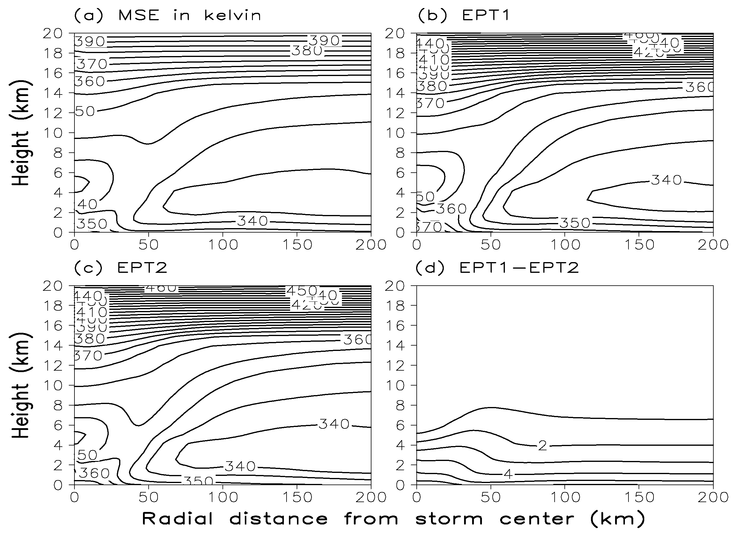
37]. As seen in
Figure 3, the symmetric structures of MSE are similar to those of
θe1 and
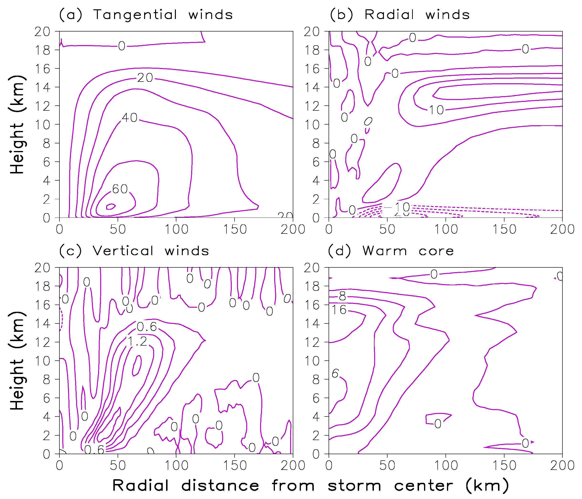
θe2. In the low-level inflow layer, MSE and
θe increase inward rapidly in the eyewall region (
Figure 2), an indication of the inflow air continually acquiring energy from the underlying ocean. This leads to a local maximum in the low-level storm center. In the upper troposphere (above approximately 14 km), all terms increase upward and have large values relative to other regions. Either
θe1 or
θe2 appears to be a good alternative to represent the primary characteristics of MSE. Nonetheless, there are still some differences between these terms. A notable feature is that the vertical gradient of MSE in the upper troposphere is much smaller than that of
θe1 and
θe2. The specific values in
θe1 and
θe2 are larger than those in MSE over the whole region. This could be because the kinetic energy generation term has been neglected in MSE [
26]. There is also a large difference between
θe1 and
θe2, more pronounced at low levels (
Figure 3d). The difference increases to as large as 6 K near the surface. This could be because many simplifications have been made in the derivation of
θe2, while the value of
θe1 is close to the real
θe.
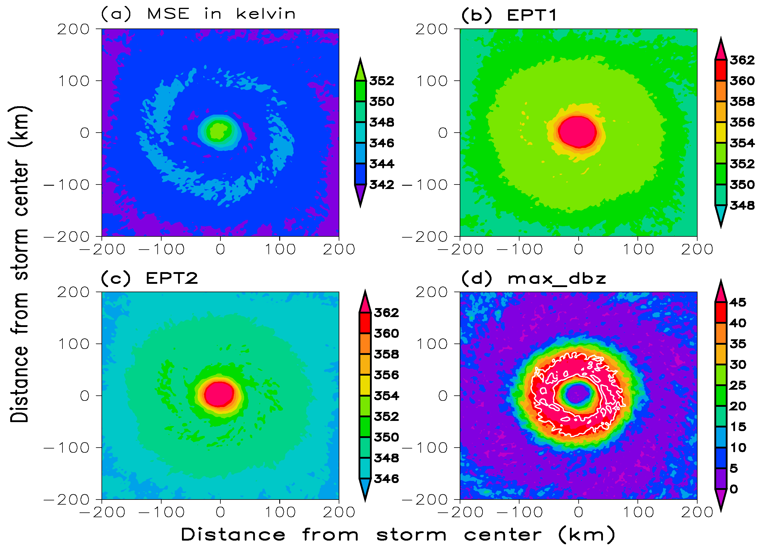
Figure 4 displays plan views of the boundary-layer MSE,
θe1,
θe2, and simulated maximum radar reflectivity. For simplicity, a height of 1 km is taken as near the top of the boundary layer [
38]. As shown in
Figure 3, there is a maximum in the storm center for MSE,
θe1, and
θe2. Again, the MSE values are noticeably lower than those of
θe1 and
θe2. A prominent feature in
Figure 4a is that the maximum MSE in the storm center is surrounded by a ring of low values immediately outside the eyewall. As a contrast,
θe in
Figure 4b a,c monotonically decreases outward from the storm center, indicating that the calculated
θe cannot fully capture the details of MSE in the boundary layer. This may lead to misinterpretation of the boundary-layer energy exchange between the inner-core and outer-core regions when MSE is assumed to be equivalent to
θe. The cold pool of MSE basically overlaps with the strongest radar reflectivity region (
Figure 4d). It is thereby speculated that low MSE values are associated with precipitation-induced cooling. Such low-MSE air, if it invades into the eyewall before recovery, could undermine the energy cycle, which will inevitably result in decreased storm intensity [
18]. In the interchangeable approximation between MSE and
θe, the rate of change in temperature following air motion is underestimated (see
Appendix A). As such,
θe cannot sufficiently incorporate such behavior of MSE, revealing that the substitution of
θe by MSE could be problematic.
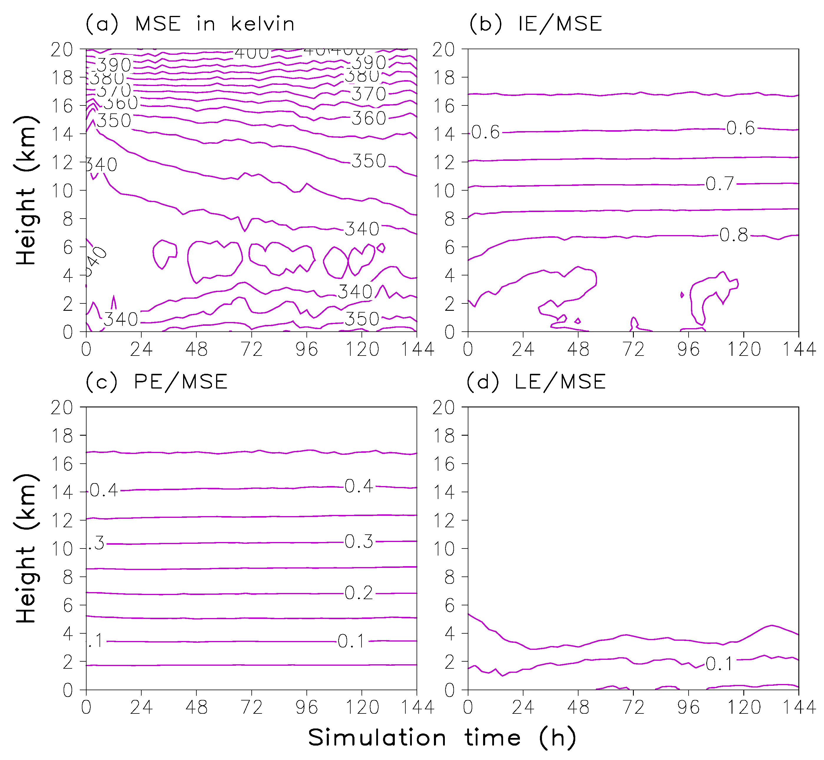
MSE in the eye region increases steadily as the storm intensifies (
Figure 5a). There are mainly two mechanisms responsible for the increased MSE. One is enhancement of MSE from the upper troposphere, which is probably associated with warming of the troposphere caused by energy conversion in TCs [
1,
2,
3]. The second is upward propagation from the ocean surface, which should arise from continuous upward transfer of heat fluxes.
Figure 5 shows the respective contributions of IE, PE, and LE to the whole MSE. IE is most pronounced at low levels, accounting for about 90% of MSE (
Figure 5b). The ratio decreases with height to about 0.5, corresponding to the steady increase in the vertical of PE (
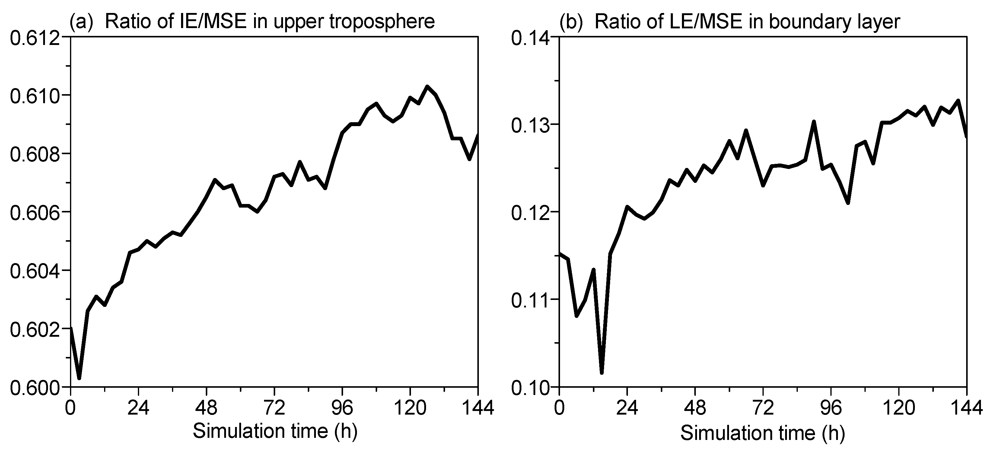
Figure 5b). As expected, because water vapor in the troposphere decreases sharply with height, the contributions of LE are discernable only at low levels, with ratios lower than 0.15. Overall, the respective contributions of the component changes vary slightly with the storm development. The evolution of their specific contributions was further investigated at the upper and lower levels (
Figure 6). In the upper troposphere, the relative importance of IE increases as the storm strengthens (
Figure 6a), concurring with the evolutionary trend of MSE. Consequently, the other two components, PE and LE, contribute less or have no discernable change (not shown). In the boundary layer, LE contributes positively to increased MSE (
Figure 6b), whereas changes in the contributions of the other two terms are negligible (not shown). This indicates that IE is dominant in enhancing MSE in the upper troposphere, and LE is dominant in the boundary layer. The behavior of MSE and each component was also investigated in other regions, including the eyewall (around the radius of maximum wind speed) and outer-core regions. Results are overall consistent with those in the eye region (not shown), implying that the above conclusion is suitable for the whole TC region.
4. Column MSE Budget
While the vertical integral of the
θe budget in TCs has been evaluated in previous studies [
36], the analysis above indicates that it may fully represent the behavior of MSE. Hence Equations (3), (5), and (6) are employed in this section to investigate the MSE budget over the whole atmosphere layer, the boundary inflow layer, and the upper outflow layer, respectively. An average time period of 108–120 h was examined while the simulated storm remained steady.
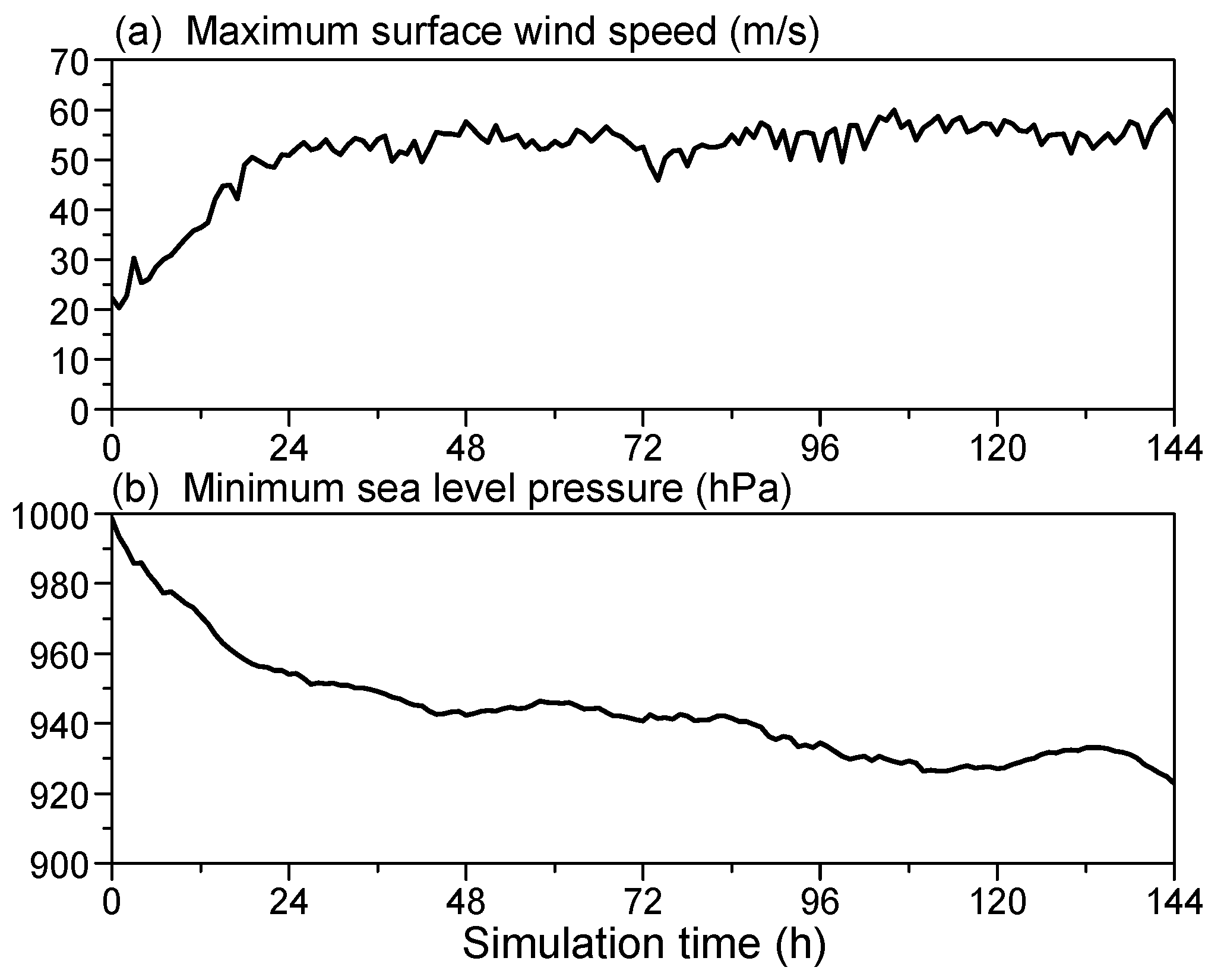
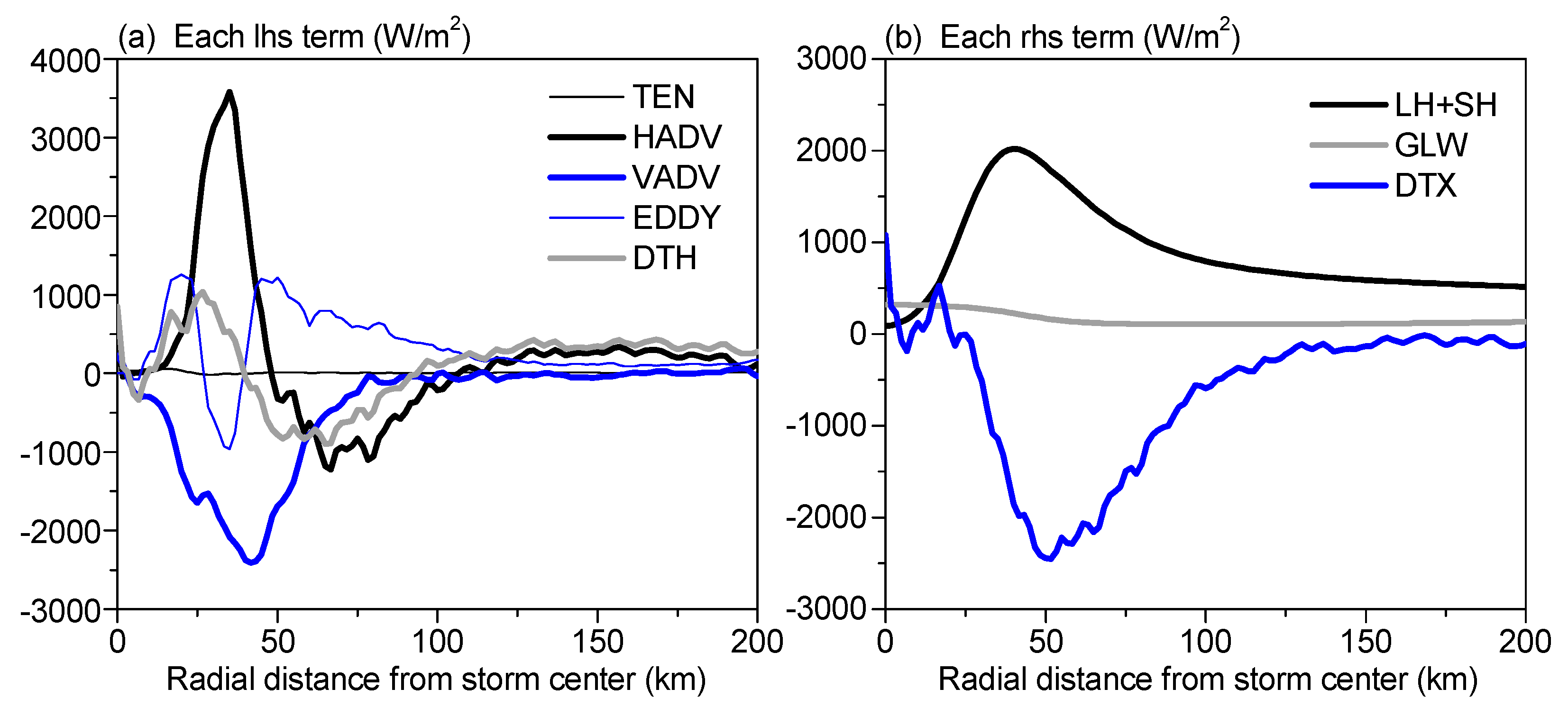
Figure 7 shows composite radial distributions of all terms in the boundary-layer MSE budget. As expected, the local tendency of MSE is negligible relative to other terms since the storm intensity evolves slowly during this time period (
Figure 1). HADV is most significant inside a radius of 50 km, that is, in the eyewall region, where the rate of radial change in MSE is large and the radial inflow is intense (
Figure 2c and
Figure 3a). Of interest is that in the region where the radius ranges from approximately 50 to 100 km, HADV is uniformly negative with values reaching −1000 W m
−2, indicating that the high MSE values following boundary-layer air parcels will be undermined before entering the eyewall under horizontal advection of radial inflow. From a radius of 100 km outward, HADV returns to positive values, but much smaller than in the inner core, indicating that MSE of inflow air increases slowly inward. As the upward motion in TCs is only active where the convection is present, VADV is analogously small in the periphery of the storm but remarkable in the inner core. It contributes negatively to the energy budget in the boundary layer, with peak values exceeding −2000 W m
−2, implying that MSE is removed from the boundary layer into the lower troposphere via ascending flow. EDDY is positive both inside and outside the eyewall, but is negative under the eyewall (approximately 25–40 km). The former should be related to air mixing and exchange between the eye and the eyewall, while the latter is associated with downward entrainment of air at the boundary layer top [
39]. Under the effects of these four processes, the net MSE changes are positive inside the eyewall and in the periphery but negative immediately outside the eyewall, approximately within a radius of 40–100 km. This suggests that in some regions of the TC, the boundary-layer MSE does not increase uniformly before the storm decays, which is apparently different from the
θe behavior.
The surface heat fluxes are significant in the eyewall region where the surface winds are the strongest (
Figure 7b). The surface heat fluxes are shown to be the dominant energy source, evidencing one of the two mechanisms enhancing MSE (
Figure 5a). Comparatively, the downward long-wave radiation fluxes at the ground surface can be neglected, though in the eye region these are slightly larger due to the absence of deep clouds. The fluxes at the boundary-layer top are computed as a residual of Equation (5). The computational bias will be discussed later. As seen in
Figure 7b, a considerable part of MSE extracted from the ocean has been transported from the boundary layer into the troposphere to fuel the TC engine. The peak values of upward propagation occur outside the eyewall, similar to the
θe budget in Ma et al. [
12]. Of interest is that the upward fluxes at the top of the boundary layer overtake the surface fluxes in the cold pool of MSE, which could lead to a decreased boundary-layer MSE in that region, as shown in
Figure 7a.
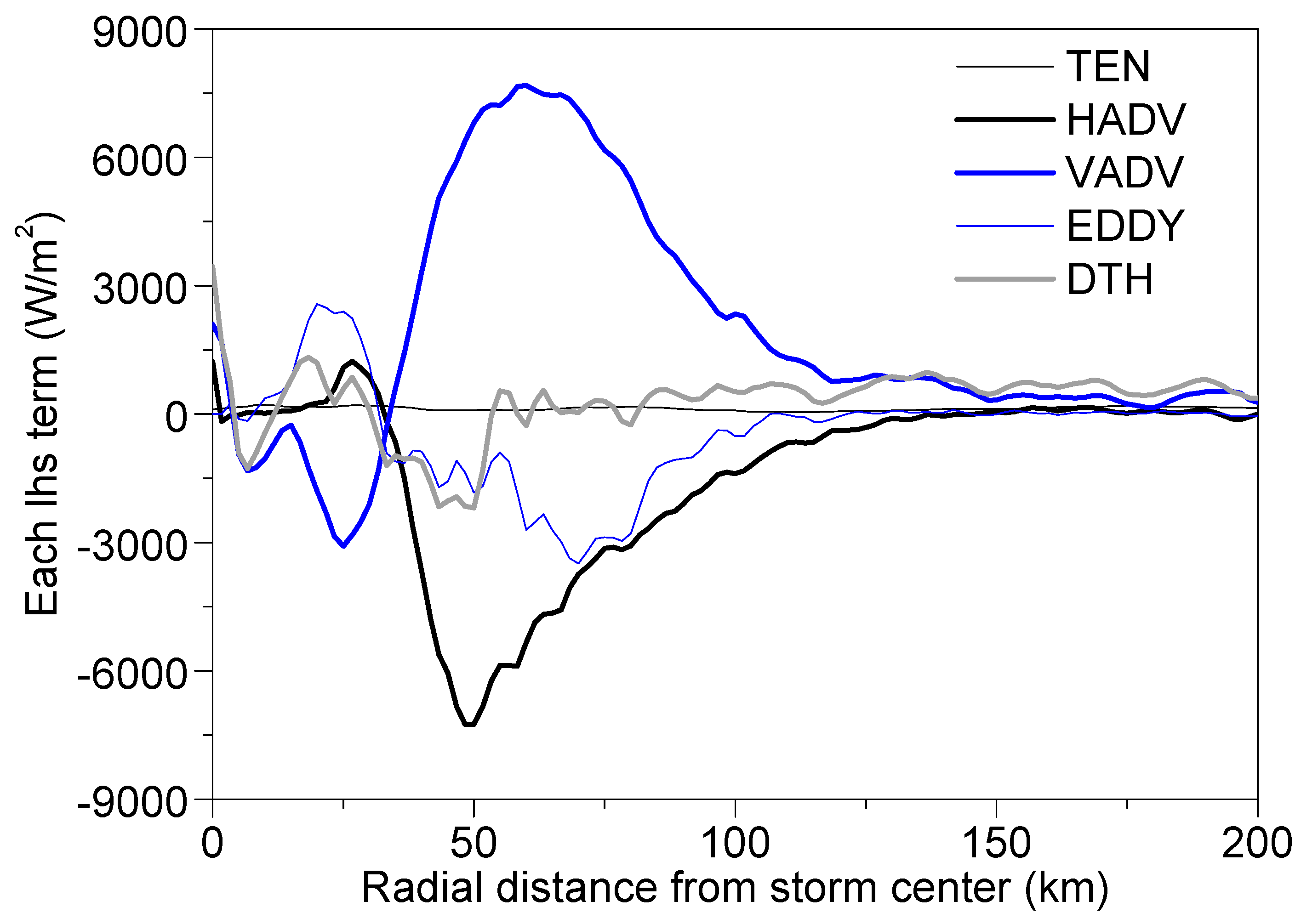
The budget of MSE in the upper troposphere is shown in
Figure 8. The budget is integrated over a depth of about 10 km (from 10 km to the top of the model domain), but the peak values of the terms are smaller than those in the boundary layer owing to slower three-dimensional winds in the upper troposphere. Another common feature is the outward shift of peak values, which is caused by the outward tilt of the eyewall (
Figure 2c). HADV is negative over the whole region, thereby advecting the high MSE outward from the TC to the surrounding environment. The resolved asymmetric eddies also contribute negatively to the MSE in the outflow layer. Nonetheless, VADV produces prominently positive values, signifying the warming effects of the upper troposphere due to the upward motion, which balances the discharge of MSE by HADV and EDDY. Unlike in the boundary layer, the net MSE change shows a roughly uniform increase, though the storm intensity is steady at this time period (
Figure 1). The steady state condition of a TC was recently investigated by Smith et al. [
38]. The long-wave radiation fluxes at the top of the atmosphere are small, as expected (
Figure 8b), but have relatively large values in the eye region since deep clouds are nearly absent there. DBX is also calculated as a residual of Equation (6). The high MSE in the upper troposphere is found to be related to upward energy transport at the bottom surface, despite being distinctly smaller than that at the sea surface. In the outer region, DBX is much smaller compared to the radiation fluxes.
Figure 9 shows the vertical integral of the MSE budget over the whole atmosphere. The contributions of HADV to the column MSE are overall negative, indicating that the role of radial outflow in the upper troposphere overall overwhelms that of the radial inflow in the low level. This is presumably because the radial outflow layer is relatively deep in the TC region. The radial distributions of VADV and EDDY resemble those in the upper troposphere, also identifying the more pronounced role of the upper troposphere than the boundary layer in changing the MSE over the whole atmosphere. From the behavior of DTH, there is both recharge and discharge of MSE in different TC regions. A volume budget is conducted in the next section for a quantitative examination.
5. Volume MSE Budget
The above column budget only demonstrates how MSE is transported inside the storm region by different processes. To quantify the energy exchange between the storm and the surrounding environment, a mass-weighted volume MSE budget is conducted in this section. For the sake of obtaining the volume-integrated form, a lateral-boundary-fixed control cylindrical volume centered at the storm center (
V) is first defined. The tendency of the volume-integrated, mass-weighted MSE to translate with the storm can be written as:
Substituting Equation (3) into Equation (7) and employing the continuity equation, the conservation equation for volume MSE budget can be derived as:
where
S is the boundary surface of the control volume and
V is three-dimensional vector winds. From Equation (8), the change of mass-weighted MSE integrated over a volume relies on surface sensible and latent heat fluxes, radiation fluxes at the atmosphere bottom and top boundaries, and net fluxes of MSE across the lateral boundaries of the control volume. The lateral fluxes of MSE are obtained as the difference of the other three terms in Equation (8). Here the control cylindrical volume is defined with a height that extends from the surface up to the top of the model domain and a radius of 200 km from the storm center. A sensitivity test with a radius of 240 km gives similar results (not shown).
Looking first at the evolution of volume-averaged, mass-weighted MSE, shown in
Figure 10, some interesting features are present. In spite of continuously small fluctuations around 1.583 × 10
5 W m
−3 after the initial model spin-up, MSE does not vary by more than 0.5% throughout the simulation. As discussed above, the volume-averaged MSE itself does increase steadily as the storm strengthens (
Figure 5a). Hence, the small change of volume-averaged, mass-weighted MSE is attributed to the offsetting roles of decreasing air density. As a storm strengthens, warming and expansion of the air in the upper troposphere and stratosphere should occur [
40], accompanied by thinning of the atmosphere according to the gas law. Given that surface enthalpy fluxes should increase correlated to the storm strengthening, the mass-weighted MSE in a fixed volume is not consequently enhanced yet, which must result in more export or less input of MSE at the storm’s lateral boundaries, or more outward radiation at top and bottom of the atmosphere, as indicated by Equation (8).
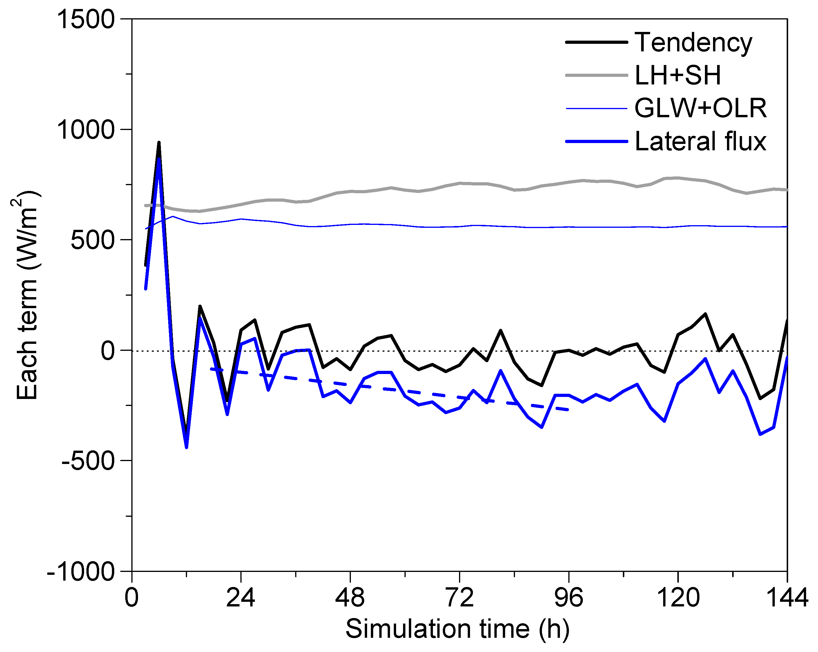
The time evolution of all terms in the volume-averaged, mass-weighted MSE budget is displayed in
Figure 11. To reduce noise with small time scales, the data were plotted every 3 h. The tendency of mass-weighted MSE changes little during the storm’s lifetime and produces near-zero values with small variation. The surface heat fluxes increase progressively until about 96 h, when the storm intensifies to a mature state, and thereafter show small temporal variation. The sum of long-wave radiation fluxes at the top and bottom of the atmosphere are nearly invariant throughout the simulation, indicating that the radiation is hardly affected by the storm intensity variation. The difference between radiation fluxes and surface heat fluxes is enlarged as the storm intensifies. Of interest is that the radiation fluxes are comparable to surface heat fluxes. This is because a cylindrical volume with a radius of 200 km is taken for the budget calculation in order to fully contain the TC regime, while in the periphery of the storm the surface enthalpy fluxes are not as large as in the inner core region due to rapidly diminished surface winds outward (
Figure 7b and
Figure 8b). The fluxes of MSE at lateral boundaries are roughly negative after an initially rapid adjustment, suggesting that the TC exports MSE throughout its lifetime, as also found by McBride [
41] from composites of rawinsonde data. The absolute values of lateral fluxes give a promisingly proportional relationship with storm intensity in that they are steadily enlarged as the storm strengthens until approximately 96 h, and thereafter are roughly around a certain threshold with fluctuations present. This indicates that the lateral export of MSE closely depends on the storm intensity. For a specified storm, the more intensified it is, the more export of MSE there tends to be. Another distinctive feature is that the fluxes of MSE by lateral export are smaller in magnitude than those by radiation, despite the radiation fluxes being negligibly small relative to other terms in the column MSE budget (
Figure 7,
Figure 8 and
Figure 9). This can be attributed to the offsetting effects among other terms at different heights. For instance, the radial outflow in the upper levels spreads large amounts of MSE outward, far exceeding the loss by radiation, which nonetheless is largely offset by the input of MSE associated with the low-level inflow air. We conducted an additional budget analysis with the radius set at 100 km, in which the lateral fluxes give larger values than, but still comparative to, the radiation fluxes (not shown).
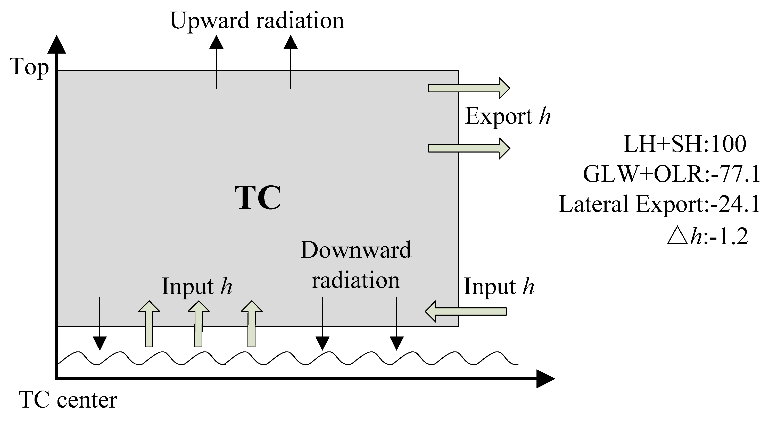
Figure 12 illustrates the conceptual schematic of the input and export of MSE in the TC system. The budget values are averaged after 24 h of simulation from the mass-weighted volume MSE budget, and then normalized by adjusting the contributions of surface enthalpy fluxes to 100. Since the input of MSE by low-level inflow has been offset by the export of MSE associated with the upper-level outflow, the surface enthalpy fluxes turn out to be the only source enhancing MSE in the TC system. A great majority of the imported MSE (77.1% in this study) is consumed by upward radiation at the top of the atmosphere and downward radiation at the surface. Only a small portion of the imported MSE (24.1%) is propagated into the surrounding environment by the radial outflow as a residual after balancing the input of MSE by the low-level inflow. Due to radiation and warming-induced expansion of the upper-level air, the mass-weighted MSE in a TC system hardly retains the recharge from sea surface or boundary inflow (with a slight deficit of −1.2% in this study), whether or not the storm is experiencing intensification or maintaining its mature state.
6. Summary
Moist static energy (MSE) is a common quantity for studying the evolution of many convective systems since it incorporates different forms of energy explicitly. In this paper, the characteristics of moist static energy in TCs are investigated on the basis of a case simulation of an idealized tropical cyclone. Since
θe is often used as an equivalence of moist static energy, a comparison of the structures of moist static energy and
θe is also performed to inspect the validity of this interchangeable approximation. Two conventionally used forms of
θe, introduced by Bolton [
35] and Rotunno and Emanuel [
36], are found to be capable of capturing the overall structure of moist static energy. However, some important features are still distorted by moist static energy. In the boundary layer, the core of high moist static energy in the TC center is surrounded by a pool of low moist static energy, which is hardly detected by both forms of
θe. Such MSE-based dry and cool air may not be sufficiently recovered before entering the eyewall updraft, thus potentially inhibiting the TC heat engine. Besides, large differences exist in the spatial gradients of moist static energy and the two forms of
θe. Caution should be used when equating
θe with moist static energy. Moist static energy is steadily enhanced as the storm strengthens. Two mechanisms are indicated to be responsible for the increased moist static energy. One is upward propagation from the sea surface, specifically the increase of LE via surface latent heat fluxes, though its contributions are only discernable at low levels. The other is warming of the upper troposphere with storm intensification, that is, increased internal energy in the upper levels.
The vertical integral of the MSE budget in the boundary layer shows that surface enthalpy fluxes are the dominant factor enhancing the MSE of the boundary layer. The horizontal advection also mostly contributes positively to the boundary layer MSE, but it plays a negative role in the low-MSE ring region, where the MSE of inflow air is diminished by precipitation-induced cooling. Overall, a considerable part of MSE extracted from the ocean is transported from the boundary layer into the troposphere, and the discharge of MSE could overwhelm its recharge in the low-MSE pool. The most significant energy exchange between the boundary layer and the troposphere aloft occurs outside the eyewall rather than right below it. The vertical integral of the MSE budget in the upper troposphere indicates that vertical advection brings in large amounts of MSE, which are mostly exported into the environment by horizontal advection. The role of radiation fluxes at the top and bottom of the atmosphere is far smaller than that of surface enthalpy fluxes near the eyewall region, but it cannot be neglected in the eye and outer storm periphery regions, where the storm winds are weak.
Unlike the volume-averaged MSE, the mass-weighted MSE in a fixed volume does not apparently increase throughout the lifetime of the simulated storm. This is because the air becomes thinner as the troposphere is steadily warmed accompanying the storm intensification. A mass-weighted volume MSE budget is further analyzed to quantify the energy exchange between the TC system and the surrounding environment. From the equation, the quantities of mass-weighted MSE in a fixed volume rely on surface enthalpy fluxes, radiation effects, and input or export of MSE at the lateral boundaries. The radiation effects are shown to depend very weakly on variation in storm intensity. The simulated TC system is found to export MSE whether or not it is undergoing intensification or maturity. It is simultaneously found that for a specified storm, the export of MSE closely relies on the storm intensity, in that the more intensified it is, the more export of MSE there tends to be. Since the input of MSE by low-level inflow is offset by the export of MSE associated with the upper-level outflow, the surface enthalpy fluxes turn to be the only source enhancing the MSE in the TC system. A great majority of the imported MSE by surface enthalpy fluxes is consumed by upward radiation at the top of the atmosphere and downward radiation at the surface, while only a small portion is transported into the surrounding environment. The input of MSE is roughly balanced by the export of MSE.
It should be mentioned that the simulated TC in this study evolved in a beneficial environment with quiescent flow and uniform sea surface temperature. Storms in the real environment should have more asymmetric MSE characteristics due to the presence of vertical wind shear, steering flow, uneven sea surface temperature, etc., and thus further real case studies are warranted. Finally, it should be noted that this study is based on an idealized simulation and the results may be quantitatively different according to variations of model configurations, resolutions, sounding profiles, and a variety of other factors.
