Abstract
This study focused on the customization of the fourth generation International Center for Theoretical Physics Regional Climate Model version 4.4 and its ability to reproduce the mean climate and most dominant modes of variability over East Africa. The simulations were performed at a spatial resolution of 25 km for the period 1998–2013. The model was driven by ERA-Interim reanalysis. The customization focus was on cumulus and microphysics schemes during the Short Rains for the year 2000. The best physics combinations were then utilized for the validation studies. The East Africa region and Lake Victoria Basin region are adapted to carry out empirical orthogonal function analysis, during the Short and Long Rains. Tropical Rainfall Measuring Mission data was utilized in the validation of the model. The first mode of variability from the model and observational data during the Short Rains was associated with the warming of the Pacific Ocean and the sea surface temperature gradients over the Indian Ocean. During the Long rains, the inter-annual rainfall variability over the Lake Victoria region was associated with the sea surface temperature anomaly over the Indian Ocean and for the East Africa region the associations were weak. The drivers during the Long Rains over East Africa region were then further investigated by splitting the season to the March–April and May periods. The March–April period was positively correlated to the West Pacific and Indian Ocean dipole index, while May was associated with the Quasi-Biennial Oscillation. In conclusion, although the model can reproduce the dominant modes of variability as in the observational data sets during the Short Rains, skill was lower during the Long Rains.
1. Introduction
The recent advancement of computational power has allowed various climate modeling groups worldwide to utilize Regional Climate Models (RCMs). Although the use of Regional Climate Models has been on the rise worldwide, a relatively limited number of studies have been conducted over East Africa. East Africa has approximately 80% of the population depending on rainfed activities [1]. In the past decades, the region has experienced numerous devastating droughts [2,3,4]. The droughts have undoubtedly caused social-economic disruption of livelihoods in the region [5] and further deterioration of the ecosystem [6,7].
Rainfall over East Africa exhibits a bimodal pattern, caused by the North-South migration of the Intertropical Convergence Zone (ITCZ). The Long Rains (March to May) are less variable and receive higher rainfall amounts compared to the Short Rains (October to December) [8]. The presence of the Africa Great Lakes, complex landscape, heterogeneous vegetation, and land cover give rise to a unique climate [9]. Early studies on inter-annual variability of precipitation over East Africa identified El Niño/Southern Oscillation (ENSO) as the leading source of variability [8,10,11] during the Short-Rains season. Later studies have shown that in addition to the teleconnection of East African precipitation with the Pacific Ocean, the Indian Ocean also plays a major role in modulating the precipitation over the region. The Indian Ocean Dipole (IOD) is a contrast between the sea surface temperature between the West and East segments of the Indian Ocean. Saji et al. [12] found evidence that the positive event of the Indian Ocean Dipole enhances rainfall over East Africa. A study done by Birkett et al. [13] found that during the 1997/1998 season, the influence of the Indian Ocean could have increased the total precipitation over the Lake Victoria Basin by 20% to 160%, while an El Niño event increased the total precipitation by about 15% to 20%.
Although the oceanic and atmospheric drivers for precipitation over East Africa are well-established for the Short-Rains season, they have remained elusive for the Long-Rains season [14]. A limited number of studies have linked ENSO to inter-annual variability of the Long Rains [15,16]. These studies have found a positive ENSO event is likely to lead to wetter conditions during the Long Rains. However, it is not the dominant force of variability during this season. Camberlin and Philippon [14] suggested that the season should not be analyzed in its entirety but rather group the onset and peak (March to April) and then analyze the cessation (May), separately.
Whereas the region has typically experienced a gradual decline in the Long Rains over the past decades, projections from the Coupled Model Intercomparison Project Phase 5 (CMIP5) models suggest that in the future, precipitation will increase over the East Africa region, a phenomenon presently identified as the “East Africa Climate paradox” [17,18]. Despite the consensus in the CMIP projections of increasing precipitation over the region, the Cook and Vizy [19] study projected a decrease in the precipitation using Regional Climate Models during the Long Rains. This apparent discrepancy necessitates the investigation of the ability of a regional climate model in producing the spatial and temporal variability of precipitation in the region.
A limited number of model customization studies have been conducted over East Africa using Regional Climate Models. Previous regional climate studies over the region include those utilizing the International Centre for Theoretical Physics (ICTP) Regional Climate Model [20,21,22,23,24,25] and some utilizing the Weather Research and Forecasting model [26,27,28,29]. This study utilizes the International Centre for Theoretical Physics (ICTP) Regional Climate Model version 4 (RegCM4). Past studies have shown the sensitivity of RCMs to dynamic configurations [20,21,22,23] necessitating the need for adequate model customization. RegCM4 includes major developments in the model physics implementation and parameterization. The implementation of a new microphysics scheme allows for a comparison on the performance of different microphysics schemes. In addition, the model allows the use of mixed cumulus schemes.
The objectives of this study are to:
- Customize the RCM, focusing on the cumulus and microphysics schemes. Prior studies have shown that inadequate treatment of clouds physics is one of the major sources of error in climate models [21,23,26,27];
- Evaluate the ability of the model to reproduce the observed inter-annual variability over the region;
- Investigate the ability of the model to reproduce the dominant modes of variability for both the Long and Short Rains.
2. Model and Experimental Setup, Data, and Methods
2.1. Model and Experimental Setup
RegCM4 is a hydrostatic, compressible, three-dimensional, regional climate model [30,31] which consists of a number of physics parameterization. A number of studies have focused on the customization of the previous versions of the RegCM model over East Africa [21,22,23,25], however, the model physics parameterization has been improved. Furthermore, there is also an implementation of a new microphysics scheme that has yet to be tested over the region. The model is utilized for customization and validation experiments. Both experiments sets are conducted at a resolution of 25 km utilizing 18 vertical levels. The domain stretches from the Atlantic to the Indian Ocean.
In the customization experiments, the simulations are divided into two key segments, the performance of cumulus schemes, and also the microphysics for the year 2000 during the Short Rains. The simulations have three months spin-up time to allow the surface and atmospheric variables to reach an equilibrium point. All simulations were done with the 1-dimensional lake model setup to be run in the tropics, Biosphere–Atmosphere Transfer Scheme version 1e (BATS1e) land surface scheme [32], Holtslag planetary boundary layer [33], and the National Center for Atmospheric Research Community Climate Model (CCM3) radiation scheme [34] as the common schemes for all the experiments. The first experiments focus on cumulus schemes. We chose the cumulus schemes that have been extensively used in the region in past studies [21,23,25]. Accordingly, our study utilizes the Massachusetts Institute of Technology Emanuel (MIT-Emanuel) [35], and Grell scheme [36] with both closures that are the Arakawa–Schubert (AS) and Fritsch–Chappell (FC) closures. The microphysics scheme for the first set of experiments is the Subgrid Explicit Moisture Scheme (SUBEX) [37]. Table 1 summarizes the different cumulus physics schemes’ combination that were conducted in the current study.

Table 1.
Summary of Regional Climate Model version 4 (RegCM4.4) simulations done to test the performance of the different cumulus schemes over the region. The Land/Ocean indicate which schemes were used over land/ocean in the simulation. AS is the Arakawa–Schubert closure for Grell, FC–Fritsch–Chappell, and MIT–Massachusetts Institute of Technology.
The focus for the second set of experiments in customization was evaluation of the different microphysics schemes. Two options are available and these are SUBEX and Nogherotto–Tompkins [38]. While SUBEX has been tested over the region, to our knowledge the Nogherotto–Tompkins scheme has not yet been tested.
Initial and lateral boundary conditions were obtained from the European Centre for medium-range weather forecast (ECWMF) Reanalysis (ERA)-Interim [39,40]. The sea surface temperatures are obtained from the National Oceanic and Atmospheric Administration, produced weekly on a 1 resolution. Both the SST and lateral boundary conditions are updated every 6 h.
2.2. Data
Since the early 1990s, station density over East Africa has been declining [41,42]. This poses a challenge in model evaluations and investigating the climatic drivers of precipitation in the region. This study utilizes the Tropical Rainfall Measuring Mission (TRMM) data to overcome the gaps associated with the gridded insitu datasets over the region. We utilized the TRMM monthly dataset from 1998 to 2013, available at a spatial resolution of 0.25 [43]. TRMM data has been used for different hydro-climatology studies and evaluated against observational insitu data in various studies [44,45,46,47]. These studies have found that although there is need to further improve the processing of precipitation data from satellite, TRMM data is able to capture the spatial and temporal distribution of precipitation in the region with relatively low biases.
Meridional, zonal wind components, and sea surface temperatures from the National Centers for Environmental Prediction (NCEP) reanalysis [48] were utilized to investigate rainfall-circulation, rainfall-sea surface temperatures relationships associated with the dominant modes of regional climate variability. The data spans from 1948 to the present and is available at monthly timescales with a T62 spatial grid.
A number of indices are chosen for this study. Selection of the indices was done based on past studies [8,10,11,12,13]. The following indices were used to determine the global teleconnections with rainfall over the region by correlating the indices with the time series of the Empirical Orthogonal Function analysis.
- Nino 3 index (https://www.esrl.noaa.gov/psd/data/correlation/nina3.anom.data): Several regions of the tropical Pacific Ocean have been chosen as being important for monitoring and identifying El Niño and La Niña. The Nino 3 index spans from 150 W to 90 W, and from 5 S to 5 N.
- Dipole Mode Index (DMI, http://www.jamstec.go.jp/aplinfo/sintexf/DATA/dmi.monthly.txt): The index is used to measure the strength of the gradient between the West and East Indian Ocean. It is obtained by calculating the difference between SST anomalies in the western (50 E to 70 E and 10 S to 10 N) and eastern (90 E to 11 E and 10 S to 0 S) equatorial Indian Ocean.
- The quasi-biennial oscillation (QBO, https://www.esrl.noaa.gov/psd/data/correlation/qbo.data): The QBO is a quasi-periodic oscillation of the equatorial 30 mb zonal wind between easterlies and westerlies in the tropical stratosphere. It propagates downwards at about 1 km per month until they are dissipated at the tropical tropopause.
- North Atlantic Oscillation (NAO, https://www.esrl.noaa.gov/psd/data/correlation/nao.data): The daily NAO index is constructed by projecting the daily (00Z) 500 mb height anomalies over the Northern Hemisphere onto the loading pattern of the NAO.
- Tropical North Atlantic (TNA, https://www.esrl.noaa.gov/psd/data/correlation/tna.data) Index: The index is calculated using sea surface temperatures (55 W–15 W, 5 N–25 N) in the eastern North Atlantic Ocean.
- Tropical South Atlantic (TSA, https://www.esrl.noaa.gov/psd/data/correlation/tsa.data) Index: The TSA is an indicator of the surface temperatures in the Gulf of Guinea. It is calculated using the SST box 30 W–10 E, 20 S–0 S.
- West Pacific (WP, https://www.esrl.noaa.gov/psd/data/correlation/wp.data) Index: The West Pacific index is obtained by calculating the gradient between the North Pacific and the East Pacific.
2.3. Methods of Analysis
Evaluation of the model skill for the customization experiments was done by calculating the metrics proposed by Pielke Sr [49]. These methods included standard deviation and root mean square errors (RMSE). The standard deviation is defined as follows:
where is the standard deviation, , is the individual prediction, is the average value, and N is the number of grid points in the predefined region. The standard deviation was calculated for both the observed and model data at seasonal timescales. The root mean square error are mathematically defined as follows:
where, and are the individual prediction and observations at the same grid point. According to Pielke Sr [49] methods, a model shows skill if the standard deviation of the model data is almost equal to the standard deviation of the observations but the root mean square error is smaller than the standard deviation of observations. In addition to the metrics proposed by Pielke Sr [49], the Pearson product moment pattern correlation was also calculated. The pattern correlation coefficient indicated whether the model and observations have the same patterns [50]. The pattern correlation coefficient was calculated as follows:
In order to separate the most dominant modes of variability, Empirical Orthogonal Function (EOF) decomposition was applied to the seasonal rainfall anomalies. EOF analysis was first introduced in meteorology by Lorenz [51] and is a fundamental tool that is now widely used for data reduction in meteorology and climate studies. A number of studies conducted over East Africa have used the tool to probe the physics underlying the variability of precipitation. In EOF analysis, we considered an vector time series , sampled at N discrete points in space. In this case we used the covariance matrix to conduct EOF analysis. The covariance matrix of is given by . Objective and subjective methods have been proposed for use in determining the significant eigenmodes, which include methods proposed by North et al. [52], Jolliffe [53], Overland and Preisendorfer [54], and Preisendorfer et al. [55] for objective methods and the scree plot as a subjective method. This study utilized the North et al. [52] method to retain the most significant modes of variability.
Figure 1 shows the topography and the domain utilized in conducting the simulations. Since EOF analysis is domain dependent, two regions were chosen for EOF analysis: the East Africa (EA) region, as in Schreck and Semazzi [56] and Lake Victoria Basin (LVB). The Lake Victoria region is chosen as it is the nerve centre for East Africa and supports approximately 40 million people through fisheries, agriculture, hydroelectric power, drinking water, and transportation.
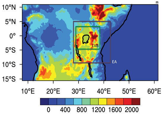
Figure 1.
Elevation (m) for the study region and domain utilized in the study. The extent of the East Africa (EA) domain (purple) and Lake Victoria Basin (LVB, green) utilized for the EOF validation analysis are shown by the rectangles.
3. Results and Discussion
The results section is divided into two major sections: Model customization and model validation.
3.1. Model Evaluation
3.1.1. Cumulus Schemes
We first presented the results on the customization experiments. RegCM model was able to capture the spatial variability (Figure 2) of precipitation over the region. Although the model can reproduce the spatial variability, there are associated biases in each cumulus scheme. The simulations utilizing the Grell AS scheme have a tendency to underestimate total precipitation (Figure 2a,b) over the whole region. The Grell FC simulation (Figure 2d,e) produced rainfall that is comparable to the observational data. Although the simulations utilizing Grell schemes underestimate total precipitation, the different closure assumptions account for the different precipitation amounts, Grell AS releases buoyant energy every time step while the Grell FC closure dissipates the buoyant energy at time scales that are approximately half an hour [57]. The simulation with the MIT-Emanuel produced excessive rainfall over mostly the Congo basin (Figure 2c,f,g). The wet bias is consistent with past studies that have shown that once the scheme is triggered it produces intense precipitation [21].
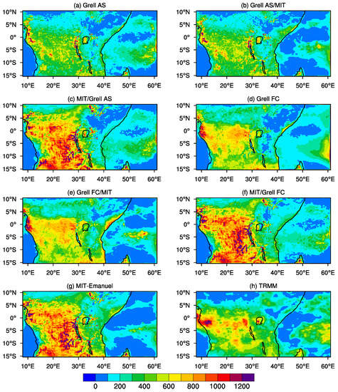
Figure 2.
Precipitation distribution (mm) using different cumulus parameterizations: (a) Grell AS; (b) Grell AS over land and MIT over ocean; (c) MIT over land and Grell AS over ocean; (d) Grell FC; (e) Grell FC over land and MIT over ocean, (f) MIT over land and Grell FC over ocean, (g) MIT; and (h) Tropical Rainfall Measuring Mission (TRMM) during the Short Rains in 2000.
The previous analysis focused on evaluating the model qualitatively by comparing the total rainfall from each of the cumulus schemes to that of the observational data, the model performance here was done utilizing the Pielke Sr [49] metrics. To analyze how the schemes perform in specific regions over the domain, the domain was subdivided based on the dominant land cover type that is the Congo rainforest (4 S–5 N, 21 E–28 E), East Africa (10 S–5 N, 28 E–42 E), and the Ocean (10 S–2 N, 42 E–58 E) regions. For the Congo rainforest, the least root mean square errors (RMSE) occurred when using the Grell FC scheme, while the highest errors occur when the MIT-Emanuel scheme is used over land (Figure 3a). In the Congo region only the simulations utilizing the Grell FC scheme, over both land and ocean shows skill. The red line in Figure 3a–c indicates the standard deviation of the TRMM datasets. The same conclusions can be drawn about the East Africa (Figure 3b) region and the ocean region (Figure 3c). The ocean region has the least skill with the RMSE for all the cumulus schemes as high as the standard deviation (Figure 3c). Zou and Zhou [58] coupled an ocean model to RegCM 3 and showed that without coupling the ocean model the atmosphere is driven by the prescribed SST forcing and hence the model does not perform well over oceans. The correlation coefficients in all the simulations are relatively high (Figure 3d), except over the oceans where the pattern correlation coefficients are as low as in the mixed convective scheme simulations. In most of the simulations, the East Africa region had higher correlations despite the cumulus scheme utilized.
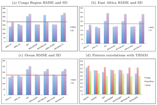
Figure 3.
Precipitation statistical evaluation for performance of the different cumulus schemes over the different regions: (a) root mean square errors (RMSE) and standard deviation over the Congo Region, (b) same as (a) but for the East Africa region, (c) same as (a) but over the ocean, and (d) pattern correlation coefficients for the different simulations with the TRMM observational data during the Short Rains in 2000.
3.1.2. Microphysics Schemes
These simulations use the same physics combinations as outlined in the previous section except for the microphysics scheme, in this case, the Nogherotto–Tompkins scheme was utilized. The mixed convective schemes were not utilized for this set of experiments as the statistics from the cumulus comparison were not superior compared to using a single cumulus scheme. The simulation utilizing the Grell AS scheme became unstable when used in combination with the Nogherotto–Tompkins scheme after running for two months. Even though the Grell FC (Figure 4a) simulation is able to capture the spatial distribution of total precipitation it has a dry bias. Using the Nogherotto–Tompkins scheme reduces the overestimation of MIT-Emanuel considerably (Figure 4b), however, the model still has a wet bias. Comparing it with the SUBEX set experiments, the Nogherotto–Tompkins schemes simulates reduced precipitation. The reduction is attributed to the lower cloud cover produced in the Nogherotto–Tompkins scheme [38].
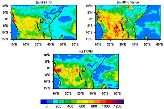
Figure 4.
Precipitation (mm) distribution using the Nogherotto–Tompkins microphysics scheme for (a) Grell FC and (b) MIT-Emanuel, and (c) TRMM during the Short Rains in 2000.
Table 2 is a summary of the statistics carried out to evaluate the microphysics scheme simulations. For the Grell FC scheme, the RMSE is less than the standard deviations of the model for all the regions. The standard deviations of the observations and model are slightly different, and we can conclude that the model shows skill. In contrast, the MIT-Emanuel scheme simulation has high standard deviations, and the RMSE are higher than the standard deviations. Hence the MIT-Emanuel scheme does not show skill in all the regions.

Table 2.
Summary of evaluation statistics for Regional Climate Model (RegCM) simulations done to test the performance of the different microphysics scheme for precipitation. RMSE is the root mean square error, SD Mod.—standard deviation calculated from model output and SD Obs.—standard deviation for observations, Cor is the pattern correlation coefficient.
The customization experiments have shown that the Grell FC produces the best statistics in terms of total rainfall over the region when either microphysics is utilized. However, comparison simulated precipitation statistics between the SUBEX and Nogherotto–Tompkins schemes shows that the simulations utilizing the SUBEX microphysics scheme had slightly superior statistics in comparison with the ones that utilized the Nogherotto–Tompkins scheme. Hence we chose the Grell FC scheme with the SUBEX microphysics scheme as the best performing scheme for this analysis and for further use in the validation analysis. In addition to this physics combination of Grell FC and SUBEX, we also utilized a well-tested parameter tuned physics combination as in Davis et al. [21]. Davis et al. [21] utilized the MIT-Emanuel scheme with the SUBEX microphysics scheme and showed that the cumulus scheme simulated the most realistic partitioning of stratiform and convective rainfall.
3.2. Model Climatology and Inter-Annual Variability
It is fundamental to test whether a RCM is able to reproduce the mean climatology and temporal variability over a region. The multiyear simulations allows us to measure the sensitivity of the model to different synoptic scale atmospheric forcings [23]. The multiyear evaluation is conducted for the period 1998 to 2013. Two physics combinations are utilized for this set, the first set with Grell FC and another with MIT Emanuel cumulus schemes. Both simulations utilized the SUBEX microphysics scheme and the other schemes are as outlined in the Model and Experimental Setup section. Figure 5 is the average seasonal rainfall for the Long Rains. The simulation utilizing Grell FC scheme generally has a dry bias, especially over Tanzania and northern Kenya in comparison with the TRMM datasets. The parameter tuned MIT-Emanuel simulation produces rainfall comparable with the observational datasets fairly well, with dry biases over northern Kenya and parts of Tanzania.
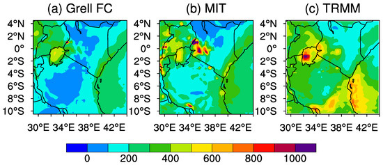
Figure 5.
Total seasonal precipitation climatology over East Africa during the Long Rains from 1998–2013 for (a) Grell FC, (b) MIT-Emanuel, and (c) TRMM.
During the Short-Rains season the model underestimates total precipitation for either physics combination (Figure 6). Dry biases are over Tanzania and northern Kenya just as in the Long-Rains case. The Grell FC simulated rainfall dry bias is generally higher than the parameter tuned MIT-Emanuel scheme during this season. Comparison on the model output for the different seasons shows that the model fails to capture enhanced rainfall during the Long-Rains season compared to the Short-Rains season. This discrepancy is consistent with analysis conducted for CMIP5 models over the region [59]. Deficiencies during this season are mostly over Tanzania and over Lake Victoria. In these regions, the model underestimates total precipitation with either model.
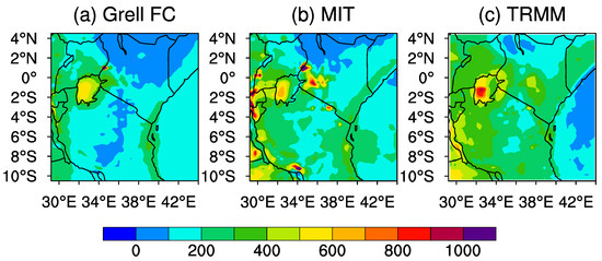
Figure 6.
Total seasonal precipitation climatology over East Africa during the Short Rains from 1998–2013 for (a) Grell FC, (b) MIT-Emanuel, and (c) TRMM.
The seasonal rainfall temporal variability is obtained by calculating the standardized anomalies and then averaging these over the East Africa region. During the Long-Rains season, the model is unable to accurately capture the inter-annual rainfall variability with correlation coefficients of and for model output of Grell FC and MIT respectively with the TRMM time series (Figure 7a). In most cases during the Long Rains, the model is unable to capture the years with extreme rainfall. For example, the model output missed some wet seasons (e.g., 2006) and dry seasons (e.g., 1999). A study conducted by Argent et al. [27] showed that in some cases the optimal physics combination during a normal year might not be optimal during an extreme year. During the OND, season the model is able to capture the inter-annual variability regardless of the cumulus scheme utilized (Figure 7b). The correlation coefficients during this season are . Although the model is able to produce rainfall very well during the Long-Rains seasons, it was unable to reproduce the correct amplitude during a positive IOD phase and El Niño year (2006).
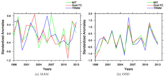
Figure 7.
Inter-annual precipitation variability for standardized seasonal rainfall anomalies over East Africa during (a) Long Rains and (b) Short Rains from 1998–2013.
From this analysis, it is clear that the model performance is better during the Short-Rains seasons than the Long-Rains seasons. Spatial qualitative analysis shows that the parameter tuned MIT-Emanuel simulation produces rainfall amounts comparable to TRMM in both seasons. For the inter-annual rainfall variability, the Grell FC simulated rainfall has higher correlation coefficients during the Long-Rains season.
3.3. Empirical Orthogonal Functional Analysis
EOF analysis was applied to seasonal rainfall. Analysis was conducted for both the Short and Long Rains utilizing the East Africa domain and the Lake Victoria Basin with the results described in the following sections.
3.3.1. Short Rains Season
We retained only the first EOF (EOF1) according to the North et al. [52] method for the East Africa region during the Short Rains. Figure 8 shows the first mode of variability for the model (Grell FC and MIT-Emanuel) and TRMM respectively. EOF1 loading during this season is dominated by one pattern, with both physics combinations producing the pattern. EOF1 from TRMM explains approximately 58% of the total variance in the region of interest while the Grell FC scheme and MIT-Emanuel scheme have a variance of 56% and 52.5%, respectively. The correlation coefficient between the TRMM EOF1 time series and those for the simulations using the Grell FC scheme and the MIT-Emanuel scheme is 0.92 and 0.90, respectively (Table 3). The time series shows alternating dry and wet years and a slightly positive trend.
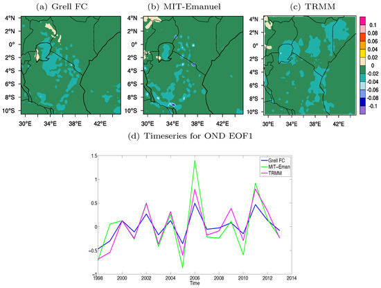
Figure 8.
Spatial and temporal distribution for Short Rains Empirical Orthogonal Function (EOF1) precipitation from the RegCM model and observation over the East Africa domain (a) Grell FC, (b) MIT Emanuel, (c) TRMM, and (d) Timeseries plot for EOF1.

Table 3.
Summary of the correlation of TRMM and model output EOF1 with the different indices used in the study for the Short Rains Season over the East Africa region. The ** indicates correlations that are statistically significant at 95% and * at 90%, significance of correlation was done using a Student’s t-test.
Pearson correlation coefficients for model and TRMM EOF1 with the different climate indices were computed. The correlation coefficients show statistically significant correlations with Nino 3 index and DMI, however DMI has a higher correlation; as compared to for Nino 3 (Table 3). All the other indices used in the study have low and statistically insignificant correlations. These results are consistent with past studies that have shown that SST anomaly forcing of the Pacific and the Indian Ocean modulate rainfall over the region [10,12,16,56,60,61,62]. A warm phase of ENSO has been shown to lead to higher precipitation over East Africa and the positive phase of IOD enhances precipitation in the region.
Composite analysis is done by considering the time series from the first EOF of TRMM. The years when the time series shows above normal rainfall are averaged to come up with the average SST and circulation patterns for the wet years. NCEP datasets are used in the composite analysis. Figure 9 is the composite for the SST and winds using the TRMM time series. Evidently Figure 9 also supports the influence of the Pacific Ocean and the Indian Ocean as in past studies. Above average rainfall is associated with the warming of the Pacific Ocean and warmer Indian Ocean temperatures along the coast of East Africa. In addition to the dipole SST over the Indian Ocean, the low level (850 hPa) wind composites show strengthening of the easterlies, hence an increase of moisture influx from the Indian Ocean.
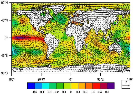
Figure 9.
Low level winds (850 hPa) and sea surface temperature anomalies composites for EOF1 during the Short Rains for enhanced rainfall over the East Africa domain using the TRMM timeseries.
For the Lake Victoria Basin, the loadings are high over the lake compared to the other regions (Figure 10). The Lake Victoria rainfall has an asymmetrical pattern that has been attributed to the lake bathymetry and the dominant flow [63]. From this EOF analysis, the model is unable to capture the asymmetrical pattern in the leading EOF, with the pattern shifted in both simulations. The correlations between the first loadings of TRMM and the model simulations are statistically significant and are 0.86 and 0.77 for Grell FC and MIT-Emanuel respectively (Table 4). EOF1 for LVB from TRMM explains approximately 58% of the total rainfall variability, while for Grell and MIT-Emanuel explains 52.8% and 48.9% respectively. Although the correlations for EOF1 with DMI is greater than 0.68 and is statistically significant, correlations with the Nino 3 index are statistically insignificant at the 95% significance level and marginally significant for TRMM and Grell FC at the 90% level.
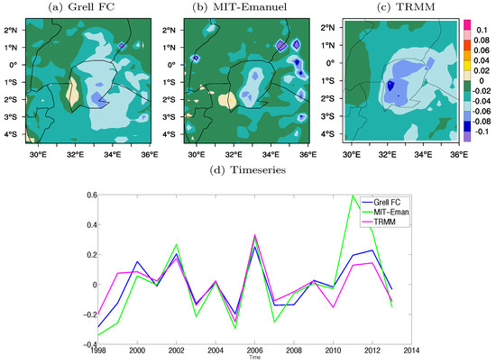
Figure 10.
Spatial and temporal distribution for Short Rains EOF1 precipitation from models and observation over Lake Victoria Basin (a) Grell FC, (b) MIT-Emannuel, (c) TRMM, and (d) timeseries plot for EOF1.

Table 4.
Summary of the correlation of TRMM and model output EOF1 with the different indices used in the study for the Short-Rains Season over the Lake Victoria Basin region. The ** indicates correlations that are statistically significant at 95% and * at 90%, significance of correlation was done using a Student’s t-test.
3.3.2. Long-Rains Season
A limited number of studies have been done on the inter-annual variability of precipitation during the Long Rains compared to the Short Rains. For the Long Rains, the association of the SSTs and their gradients with seasonal rainfall variability have not yet been established. However, some studies have indicated that the variability of the onset and peak is different from that of the cessation and hence correlating individual months with the climate indices can reveal underlying associations [14,64]. We first analyzed the Long-Rains season over the East Africa region in its entirety and then split the season into two, where the cessation was analyzed separately from the rest of the season. The spatial pattern from both the model simulations and TRMM was mostly dominated by one pattern (Figure 11). The time series does not show a trend, and the amplitudes were comparable in most years except for the MIT-Emanuel during 1997 when the amplitudes are much higher than in the observations. The first EOF explains approximately 34% for MIT Emanuel, 33.1% for Grell scheme, and 23.6% for TRMM which is much less than in the Short -Rains season, suggesting an interaction of different drivers contributing to the seasonal total rainfall.
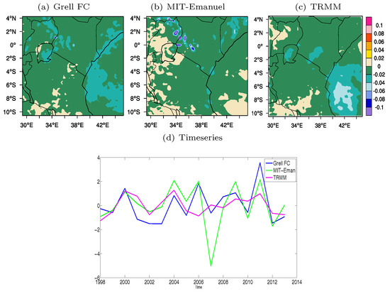
Figure 11.
Spatial and temporal distribution for Long Rains EOF1 precipitation from models and observation (a) Grell FC, (b) MIT Emanuel, (c) TRMM, and (d) timeseries plot for EOF1 over East Africa.
Correlation between both physics combinations and TRMM data are not statistically significant (Table 5), implying that during this season the model has less skill. We focused on just the TRMM correlations since the correlations with the model are very weak. During this season, the precipitation was weakly correlated with the IOD index only and all the other correlations were insignificant.

Table 5.
Summary of the correlation of TRMM and model output EOF1 with the different indices used in the study for the Long-Rains Season. The ** indicates correlations that are statistically significant at 95% and * at 90%, significance of correlation was done using a Student’s t-test.
Since a number of studies have already alluded to the fact that the drivers of precipitation in this season were temporarily distinct we adopted the temporal separation of the season suggested in Camberlin and Philippon [14]. The EOF1 for TRMM March–April explains 28% of the variability while that of MIT-Emanuel and Grell FC explains and , respectively. During the March–April time period, the Grell FC and TRMM time series were statistically correlated while that for MIT-Emanuel was insignificantly correlated. The Grell FC and TRMM time series had statistically significant correlation with the DMI at the 95% confidence level. In addition to the DMI correlation, the TRMM time series was also negatively correlated with the West Pacific index. The correlations were however weak, suggesting that a number of teleconnections do affect the precipitation during this time period. Furthermore, the first EOF only explains 28% of the variability, implying that we only explained a small percentage of the variability. Analyzing the SST and wind composites for the Indian Ocean shows warming over the East Africa coast and easterlies into the region (Figure 12).
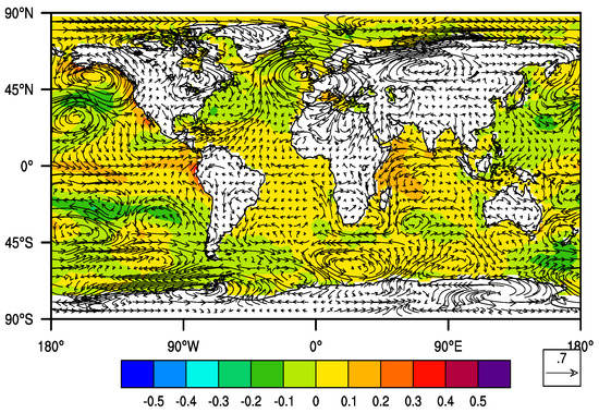
Figure 12.
Wind and sea surface temperature anomaly composites during Mar–Apr for EOF1 over East Africa region using the TRMM timeseries.
For the cessation period, the correlations for the EOF1 time series from both simulations are statistically significant with that of TRMM. Correlating these time series with climate indices showed that during the cessation, the rainfall in the region had a teleconnection with the QBO. The MIT-Emanuel scheme however is not statistically correlated with the QBO index. Indeje and Semazzi [65] created 8 different homogeneous regions and correlated them with the QBO index. Their findings revealed the heterogeneity of the region, some regions had high positive correlations while for some the correlations were low. Thus in our case, since the domain is big we expected that the signal would be diluted and weaker as we might have included other regions that were not highly modulated by the QBO.
Unlike in the case of the Short Rains, where the first EOF over the LVB from the model was not highly correlated with the observations during the Long Rains season, the model performed better over the lake. The first EOF over the basin explained approximately 52.3% for MIT-Emanuel, 50.9% for Grell FC, and 40% for TRMM (Figure 13). Both the physics scheme combination and the TRMM timeseries were correlated with the IOD index, suggesting that the drivers in the region were different (Table 5).
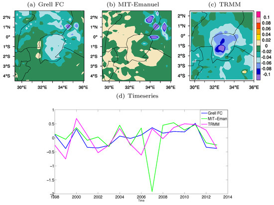
Figure 13.
Spatial and temporal distribution for Long Rains EOF1 precipitation from models and observation (a) Grell FC, (b) MIT Emanuel, (c) TRMM, and (d) timeseries plot for EOF1 over the Lake Victoria Basin.
The SST composites (Figure 14) that are produced by using the LVB time series have the same pattern as the East Africa subregion, however the intensities are different. Comparison of the SST composites for the LVB and the East Africa domain showed that the LVB domain composites had a stronger gradient in the Indian Ocean as compared to the one obtained by compositing the East Africa Long-Rains time series. This highlights the importance of analyzing the region in smaller clusters that have the same rainfall regimes. The East Africa region consists of the Southern part of the domain that has an unimodal rainfall regime, and the rest of the domain is mostly bimodal hence why the mixed effects might be difficult to separate out in EOF analysis.
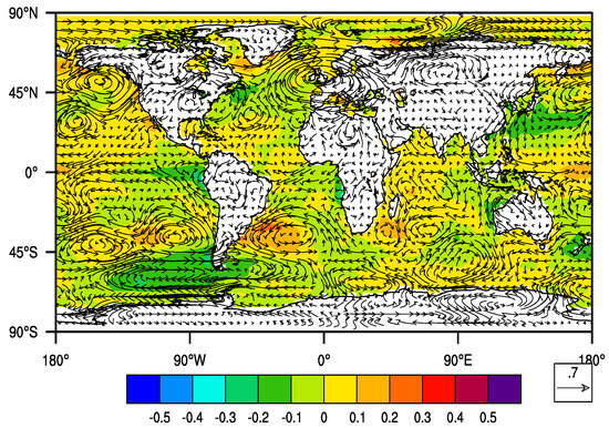
Figure 14.
Wind and sea surface temperature anomaly composites for EOF1 during the Long Rains over the Lake Victoria domain using the TRMM timeseries.
4. Summary and Conclusions
This study focused on the customization and validation of the RegCM4 model. The customization experiments focused on the cumulus and microphysics schemes. In the customization experiments, it was shown that over the domain of analysis Grell FC had the highest skills using either SUBEX or Nogherotto–Tompkins microphysics scheme. Comparison of the SUBEX and Nogherotto–Tompkins revealed that the physics combination of the MIT-Emanuel and Nogherotto–Tompkins scheme had lower wet biases in comparison with simulations that utilized the SUBEX scheme. Even though the wet bias was lower, the model still did not show skill according to Pielke Sr [49] metrics. Comparison of the SUBEX scheme and Nogherotto–Tompkins scheme revealed that in general simulations utilizing the Nogherotto–Tompkins scheme are generally drier than those utilizing the SUBEX scheme. Utilizing both the quantitative and qualitative evaluation analysis, we chose the Grell FC scheme with the SUBEX microphysics scheme as the best performing scheme for customization analysis and for further use in the validation analysis. Additionally, to the Grell FC ad SUBEX physics combination, we also utilized a well-tested parameter tuned physics combination as in Davis et al. [21], utilizing the MIT-Emanuel cumulus scheme and SUBEX microphysics scheme. The Davis et al. [21] parameter tuned physics combination was shown previously to produce the most realistic partitioning of stratiform and convective rainfall.
Validation was conducted on the seasonal total precipitation of the two physics combinations during the Short and Long Rains over East Africa. Two sets of validation analysis were conducted, (i) seasonal precipitation climatology and inter-annual variability as well as (ii) EOF precipitation seasonal analysis for both seasons. The simulated Grell FC precipitation climatology had a dry tendency for both the Long and Short-Rains season. In comparison, the parameter tuned simulated MIT-Emanuel precipitation was comparable to observed rainfall over the region. Both physics combinations failed to capture the enhanced rainfall during the Long-Rains season compared to the Short-Rains season. For inter-annual variability, model skill was found to be higher during the Short-Rains season compared to the Long Rains where the correlation coefficients were very low. From this analysis, the simulation with Grell FC could reproduce the inter-annual rainfall better than the simulation with MIT-Emanuel scheme. However, the Grell FC simulated precipitation was lower than the observed precipitation.
EOF validation analysis showed that during the Short Rains, both the physics combinations were able to reproduce the first mode of variability spatially and temporal for regional East Africa and the Lake Victoria Basin precipitation. This is especially so for the East Africa region where the model time series correlation coefficient and that for TRMM is about . When the Lake Victoria domain was considered, the correlation between the first modes for TRMM and from the model was reduced. This might imply that the model was unable to capture the mesoscale features over the lake and thus more work was required to accurately capture the dynamics over the lake. For the Short Rains, this study revealed that in recent years the inter-annual variability of precipitation over East Africa was mostly dominated by the variability of the Indian Ocean, rather than the ENSO events. This information is very critical in informing seasonal forecasting over the region. During the Long Rains, the rainfall was weakly associated with the SST gradients over the Indian Ocean. However, for the Lake Victoria Basin region, the correlation coefficients were relatively high, highlighting the importance of investigating the drivers for smaller homogeneous regions. Splitting the season into two, the onset and peak, and cessation revealed some underlying drivers. The March–April (onset–peak) period is positively correlated to the West Pacific with the TRMM datasets, however, both model simulations fail to capture the contribution of the West Pacific. The West Pacific has been linked to East Africa through modification of the Walker Circulation. During the cessation period, the QBO indices were significantly correlated to the EOF1 time series. The positive phase of the QBO was linked to enhanced rainfall over the region and has been identified as one of the sub-seasonal drivers of rainfall over the region. In addition to the West Pacific, other studies have identified the role of the Atlantic Ocean in modulating the cessation over the East Africa region.
In conclusion, although the model could simulate the dominant modes of variability during the Short Rains as in the TRMM dataset, the model had less skill during the Long Rains, especially when the East Africa domain is considered. More work needs to be done to understand the physical mechanisms that drive the Long-Rains season. The Grell FC scheme, despite its dry bias, can reproduce the inter-annual and the dominant modes of variability over the region for both seasons better than the MIT-Emanuel scheme. Hence we recommend using the Grell FC over the region, although parameter tuning needs to be conducted in order to correct the dry bias.
Author Contributions
Conceptualization, M.G. and F.H.M.S.; Formal analysis, M.G.; Supervision, F.H.M.S.; Writing original draft, M.G.; Writing review and editing, M.G. and F.H.M.S.
Funding
This research was funded by the Schlumberger Faculty for the Future Fellowship and the International Peace Scholarship.
Acknowledgments
This study is part of the PhD work for M.G. at North Carolina State University, Raleigh, North Carolina. All the simulations were conducted on the NCAR Yellowstone supercomputing system with analysis conducted using the NCAR Command Language.
Conflicts of Interest
The authors declare no conflict of interest.
References
- East African Community. Agriculture and Rural Development Policy for the East African Community; East African Community: Arusha, Tanzania, 2006. [Google Scholar]
- Yang, W.; Seager, R.; Cane, M.A.; Lyon, B. The East African long rains in observations and models. J. Clim. 2014, 27, 7185–7202. [Google Scholar] [CrossRef]
- Lyon, B.; DeWitt, D.G. A recent and abrupt decline in the East African long rains. Geophys. Res. Lett. 2012, 39. [Google Scholar] [CrossRef]
- Williams, A.P.; Funk, C. A westward extension of the warm pool leads to a westward extension of the Walker circulation, drying eastern Africa. Clim. Dyn. 2011, 37, 2417–2435. [Google Scholar] [CrossRef]
- Hillier, D.; Dempsey, B. A Dangerous delay: The cost of late response to early warnings in the 2011 drought in the Horn of Africa. Oxfam Policy Pract. Agric. Food Land 2012, 12, 1–34. [Google Scholar]
- Robinson, S.; Nishimizu, M. Africa-Second Phase of the Lake Victoria Environmental Management Project; World Development Sources: Washington, DC, USA, 2015. [Google Scholar]
- Tenge, A.J.; Mvuma, A.N.; Baker, S.B.; Mongi, H.J.; Mwakijele, J.; Gabriel, M.C. Community Perception on Lake Victoria Basin Resources Degradation: Implications to Sustainable Management. J. Sustain. Dev. 2015, 8, 14. [Google Scholar] [CrossRef]
- Mutai, C.; Ward, M.; Colman, A. Towards the prediction of the East Africa short rains based on sea-surface temperature–atmosphere coupling. Int. J. Climatol. 1998, 18, 975–997. [Google Scholar] [CrossRef]
- Anyah, R.O.; Semazzi, F.H.; Xie, L. Simulated physical mechanisms associated with climate variability over Lake Victoria Basin in East Africa. Mon. Weather Rev. 2006, 134, 3588–3609. [Google Scholar] [CrossRef]
- Ogallo, L. Relationships between seasonal rainfall in East Africa and the Southern Oscillation. J. Climatol. 1988, 8, 31–43. [Google Scholar] [CrossRef]
- Nicholson, S.E.; Kim, J. The relationship of the El Nino-Southern oscillation to African rainfall. Int. J. Climatol. 1997, 17, 117–135. [Google Scholar] [CrossRef]
- Saji, N.; Goswami, B.N.; Vinayachandran, P.; Yamagata, T. A dipole mode in the tropical Indian Ocean. Nature 1999, 401, 360–363. [Google Scholar] [CrossRef]
- Birkett, C.; Murtugudde, R.; Allan, T. Indian Ocean climate event brings floods to East Africa’s lakes and the Sudd Marsh. Geophys. Res. Lett. 1999, 26, 1031–1034. [Google Scholar] [CrossRef]
- Camberlin, P.; Philippon, N. The East African March-May rainy season: Associated atmospheric dynamics and predictability over the 1968-97 period. J. Clim. 2002, 15, 1002–1019. [Google Scholar] [CrossRef]
- Ntale, H.K.; Gan, T.Y. East African rainfall anomaly patterns in association with El Nino/Southern Oscillation. J. Hydrol. Eng. 2004, 9, 257–268. [Google Scholar] [CrossRef]
- Indeje, M.; Semazzi, F.H.; Ogallo, L.J. ENSO signals in East African rainfall seasons. Int. J. Climatol. 2000, 20, 19–46. [Google Scholar] [CrossRef]
- Semazzi, H.; Cornforth, R.; Houghton-Carr, H.; Bain, C.; Anyah, R.; Roberts, R.; Xie, L.; Ogallo, L.; Waniha, P.; Githeko, A.; et al. HyVic Science Plan. Available online: http://climlab.meas.ncsu.edu/HYVIC/HYVIC\protect\discretionary{\char\hyphenchar\font}{}{}Science_Plan.pdf (accessed on 10 October 2018).
- Rowell, D.P.; Booth, B.B.; Nicholson, S.E.; Good, P. Reconciling past and future rainfall trends over east Africa. J. Clim. 2015, 28, 9768–9788. [Google Scholar] [CrossRef]
- Cook, K.H.; Vizy, E.K. Projected changes in East African rainy seasons. J. Clim. 2013, 26, 5931–5948. [Google Scholar] [CrossRef]
- Sun, L.; Semazzi, F.H.; Giorgi, F.; Ogallo, L. Application of the NCAR regional climate model to eastern Africa: 1. Simulation of the short rains of 1988. J. Geophys. Res. Atmos. 1999, 104, 6529–6548. [Google Scholar] [CrossRef]
- Davis, N.; Bowden, J.; Semazzi, F.; Xie, L.; Önol, B. Customization of RegCM3 regional climate model for eastern Africa and a tropical Indian Ocean domain. J. Clim. 2009, 22, 3595–3616. [Google Scholar] [CrossRef]
- Anyah, R.O.; Semazzi, F.H. Variability of East African rainfall based on multiyear RegCM3 simulations. Int. J. Climatol. 2007, 27, 357–371. [Google Scholar] [CrossRef]
- Segele, Z.T.; Leslie, L.M.; Lamb, P.J. Evaluation and adaptation of a regional climate model for the Horn of Africa: rainfall climatology and interannual variability. Int. J. Climatol. 2009, 29, 47–65. [Google Scholar] [CrossRef]
- Sylla, M.B.; Coppola, E.; Mariotti, L.; Giorgi, F.; Ruti, P.; DellAquila, A.; Bi, X. Multiyear simulation of the African climate using a regional climate model (RegCM3) with the high resolution ERA-interim reanalysis. Clim. Dyn. 2010, 35, 231–247. [Google Scholar] [CrossRef]
- Ogwang, B.A.; Chen, H.; Li, X.; Gao, C. Evaluation of the capability of RegCM4. 0 in simulating East African climate. Theor. Appl. Climatol. 2015, 124, 303–313. [Google Scholar] [CrossRef]
- Pohl, B.; Crétat, J.; Camberlin, P. Testing WRF capability in simulating the atmospheric water cycle over Equatorial East Africa. Clim. Dyn. 2011, 37, 1357–1379. [Google Scholar] [CrossRef]
- Argent, R.; Sun, X.; Semazzi, F.; Xie, L.; Liu, B. The development of a customization framework for the WRF Model over the Lake Victoria basin, Eastern Africa on seasonal timescales. Adv. Meteorol. 2015, 2015, 653473. [Google Scholar] [CrossRef]
- Sun, X.; Xie, L.; Semazzi, F.; Liu, B. Effect of lake surface temperature on the spatial distribution and intensity of the precipitation over the Lake Victoria basin. Mon. Weather Rev. 2015, 143, 1179–1192. [Google Scholar] [CrossRef]
- Abdelwares, M.; Haggag, M.; Wagdy, A.; Lelieveld, J. Customized framework of the WRF model for regional climate simulation over the Eastern NILE basin. Theor. Appl. Climatol. 2018, 134, 1135–1151. [Google Scholar] [CrossRef]
- Giorgi, F.; Coppola, E.; Solmon, F.; Mariotti, L.; Sylla, M.; Bi, X.; Elguindi, N.; Diro, G.; Nair, V.; Giuliani, G.; et al. RegCM4: Model description and preliminary tests over multiple CORDEX domains. Clim. Res. 2012, 2, 7–29. [Google Scholar] [CrossRef]
- Giorgi, F.; Anyah, R. The road towards RegCM4. Clim. Res. 2012, 52, 3–6. [Google Scholar] [CrossRef]
- Dickinson, E.; Henderson-Sellers, A.; Kennedy, J. Biosphere-Atmosphere Transfer Scheme (BATS) Version 1E as Coupled to the NCAR Community Climate Model; NCAR: Boulder, CO, USA, 1993. [Google Scholar]
- Holtslag, A.; De Bruijn, E.; Pan, H. A high resolution air mass transformation model for short-range weather forecasting. Mon. Weather Rev. 1990, 118, 1561–1575. [Google Scholar] [CrossRef]
- Kiehl, T.; Hack, J.; Bonan, B.; Boville, A.; Briegleb, P.; Williamson, L.; Rasch, J. Description of the NCAR Community Climate Model (CCM3); NCAR: Boulder, CO, USA, 1996. [Google Scholar]
- Emanuel, K.A. A scheme for representing cumulus convection in large-scale models. J. Atmos. Sci. 1991, 48, 2313–2329. [Google Scholar] [CrossRef]
- Grell, G.A. Prognostic evaluation of assumptions used by cumulus parameterizations. Mon. Weather Rev. 1993, 121, 764–787. [Google Scholar] [CrossRef]
- Pal, J.S.; Small, E.E.; Eltahir, E.A. Simulation of regional-scale water and energy budgets: Representation of subgrid cloud and precipitation processes within RegCM. J. Geophys. Res. Atmos. 2000, 105, 29579–29594. [Google Scholar] [CrossRef]
- Nogherotto, R.; Tompkins, A.M.; Giuliani, G.; Coppola, E.; Giorgi, F. Numerical framework and performance of the new multiple-phase cloud microphysics scheme in RegCM4. 5: Precipitation, cloud microphysics, and cloud radiative effects. Geosci. Model Dev. 2016, 9, 2533–2547. [Google Scholar] [CrossRef]
- Dee, D.; Uppala, S.; Simmons, A.; Berrisford, P.; Poli, P.; Kobayashi, S.; Andrae, U.; Balmaseda, M.; Balsamo, G.; Bauer, P.; et al. The ERA-Interim reanalysis: Configuration and performance of the data assimilation system. Q. J. R. Meteorol. Soc. 2011, 137, 553–597. [Google Scholar] [CrossRef]
- Simmons, A.; Uppala, S.; Dee, D.; Kobayashi, S. ERA-Interim: New ECMWF reanalysis products from 1989 onwards. ECMWF Newslett. 2007, 110, 25–35. [Google Scholar]
- Becker, A.; Finger, P.; Meyer-Christoffer, A.; Rudolf, B.; Schamm, K.; Schneider, U.; Ziese, M. A description of the global land-surface precipitation data products of the Global Precipitation Climatology Centre with sample applications including centennial (trend) analysis from 1901—Present. Earth Syst. Sci. Data 2013, 5, 71–99. [Google Scholar] [CrossRef]
- Funk, C.; Nicholson, S.E.; Landsfeld, M.; Klotter, D.; Peterson, P.; Harrison, L. The centennial trends greater horn of Africa precipitation dataset. Sci. Data 2015, 2, 150050. [Google Scholar] [CrossRef]
- Huffman, G.; Bolvin, D. TRMM and Other Data Precipitation Data Set Documentation; Laboratory for Atmospheres, NASA Goddard Space Flight Center and Science Systems and Applications, Inc.: Washington, DC, USA, 2011.
- Dinku, T.; Ceccato, P.; Grover-Kopec, E.; Lemma, M.; Connor, S.; Ropelewski, C. Validation of satellite rainfall products over East Africa’s complex topography. Int. J. Remote Sens. 2007, 28, 1503–1526. [Google Scholar] [CrossRef]
- Li, L.; Hong, Y.; Wang, J.; Adler, R.F.; Policelli, F.S.; Habib, S.; Irwn, D.; Korme, T.; Okello, L. Evaluation of the real-time TRMM-based multi-satellite precipitation analysis for an operational flood prediction system in Nzoia Basin, Lake Victoria, Africa. Nat. Hazards 2009, 50, 109–123. [Google Scholar] [CrossRef]
- Duan, Z.; Bastiaanssen, W. First results from Version 7 TRMM 3B43 precipitation product in combination with a new downscaling—Calibration procedure. Remote Sens. Environ. 2013, 131, 1–13. [Google Scholar] [CrossRef]
- Naumann, G.; Barbosa, P.; Carrao, H.; Singleton, A.; Vogt, J. Monitoring drought conditions and their uncertainties in Africa using TRMM data. J. Appl. Meteorol. Climatol. 2012, 51, 1867–1874. [Google Scholar] [CrossRef]
- Kalnay, E.; Kanamitsu, M.; Kistler, R.; Collins, W.; Deaven, D.; Gandin, L.; Iredell, M.; Saha, S.; White, G.; Woollen, J.; et al. The NCEP/NCAR 40-year reanalysis project. Bull. Am. Meteorol. Soc. 1996, 77, 437–471. [Google Scholar] [CrossRef]
- Pielke Sr, R.A. Mesoscale Meteorological Modeling; Academic Press: Cambridge, MA, USA, 2013; Volume 98. [Google Scholar]
- Taylor, K.E. Summarizing multiple aspects of model performance in a single diagram. J. Geophys. Res. Atmos. 2001, 106, 7183–7192. [Google Scholar] [CrossRef]
- Lorenz, E.N. Empirical Orthogonal Functions and Statistical Weather Prediction; Statistical Forecasting Project: Cambridge, MA, USA, 1956. [Google Scholar]
- North, G.R.; Bell, T.L.; Cahalan, R.F.; Moeng, F.J. Sampling errors in the estimation of empirical orthogonal functions. Mon. Weather Rev. 1982, 110, 699–706. [Google Scholar] [CrossRef]
- Jolliffe, I.T. Discarding variables in a principal component analysis. I: Artificial data. Appl. Stat. 1972, 21, 160–173. [Google Scholar] [CrossRef]
- Overland, J.E.; Preisendorfer, R. A significance test for principal components applied to a cyclone climatology. Mon. Weather Rev. 1982, 110, 1–4. [Google Scholar] [CrossRef]
- Preisendorfer, R.W.; Zwiers, F.; Barnett, T. Foundations of principal component selection rules. SIO Ref. Ser. 1981, 192, 10005106368. [Google Scholar]
- Schreck, C.J.; Semazzi, F.H. Variability of the recent climate of eastern Africa. Int. J. Climatol. 2004, 24, 681–701. [Google Scholar] [CrossRef]
- Giorgi, F.; Shields, C. Tests of precipitation parameterizations available in latest version of NCAR regional climate model (RegCM) over continental United States. J. Geophys. Res. Atmos. 1999, 104, 6353–6375. [Google Scholar] [CrossRef]
- Zou, L.; Zhou, T. Can a regional ocean–atmosphere coupled model improve the simulation of the interannual variability of the western North Pacific summer monsoon? J. Clim. 2013, 26, 2353–2367. [Google Scholar] [CrossRef]
- Yang, W.; Seager, R.; Cane, M.A.; Lyon, B. The rainfall annual cycle bias over East Africa in CMIP5 coupled climate models. J. Clim. 2015, 28, 9789–9802. [Google Scholar] [CrossRef]
- Black, E.; Slingo, J.; Sperber, K.R. An observational study of the relationship between excessively strong short rains in coastal East Africa and Indian Ocean SST. Mon. Weather Rev. 2003, 131, 74–94. [Google Scholar] [CrossRef]
- Bowden, J.H.; Semazzi, F.H. Empirical analysis of intraseasonal climate variability over the Greater Horn of Africa. J. Clim. 2007, 20, 5715–5731. [Google Scholar] [CrossRef]
- Manatsa, D.; Chipindu, B.; Behera, S.K. Shifts in IOD and their impacts on association with East Africa rainfall. Theor. Appl. Climatol. 2012, 110, 115–128. [Google Scholar] [CrossRef]
- Anyah, R.O.; Semazzi, F. Idealized simulation of hydrodynamic characteristics of Lake Victoria that potentially modulate regional climate. Int. J. Climatol. 2009, 29, 971–981. [Google Scholar] [CrossRef]
- Nicholson, S.E. The Predictability of Rainfall over the Greater Horn of Africa. Part II: Prediction of Monthly Rainfall during the Long Rains. J. Hydrometeorol. 2015, 16, 2001–2012. [Google Scholar] [CrossRef]
- Indeje, M.; Semazzi, F. Relationships between QBO in the lower equatorial stratospheric zonal winds and East African seasonal rainfall. Meteorol. Atmos. Phys. 2000, 73, 227–244. [Google Scholar] [CrossRef]
© 2019 by the authors. Licensee MDPI, Basel, Switzerland. This article is an open access article distributed under the terms and conditions of the Creative Commons Attribution (CC BY) license (http://creativecommons.org/licenses/by/4.0/).