Article

Spatiotemporal Change of Plum Rains in the Yangtze River Delta and Its Relation with EASM, ENSO, and PDO During the Period of 1960–2012

1
Key Laboratory of Geographic Information Science (Ministry of Education), East China Normal University, Shanghai 200241, China
2
Research Center for East-West Cooperation in China, East China Normal University, Shanghai 200241, China
3
School of Geographic Sciences, East China Normal University, Shanghai 200241, China
4
School of Urban and Geography, Lanzhou City College, Lanzhou 730070, China
5
Jianhu Data Technology (Shanghai) Co., Ltd, Shanghai 201700, China
6
Faculty of Tourism Management, Shanxi University of Finance & Economics, Taiyuan 030006, China
*
Author to whom correspondence should be addressed.
Atmosphere 2019, 10(5), 258; https://doi.org/10.3390/atmos10050258
Submission received: 16 April 2019 / Revised: 5 May 2019 / Accepted: 7 May 2019 / Published: 9 May 2019
(This article belongs to the Special Issue Lower Atmosphere Meteorology)

Abstract

:
The Plum Rains process is a complex process, and its spatiotemporal variations and influencing factors on different time scales still need further study. Based on a dataset on the Plum Rains in the Yangtze River Delta, from 33 meteorological stations during the period of 1960 to 2012, we investigated the spatiotemporal variations of Plum Rains and their relation with the East Asian Summer Monsoon (EASM), the El Niño-Southern Oscillation (ENSO), and the Pacific Decadal Oscillation (PDO) using an integrated approach that combines ensemble empirical mode decomposition (EEMD), empirical orthogonal function (EOF), and correlation analysis. The main conclusions were as follows: (1) the plum rainfall (i.e., the rainfall during the period of Plum Rains) showed a trend of increasing first and then decreasing, and it had a three-year and six-year cycle on the inter-annual scale and a 13-year and 33-year cycle on the inter-decadal scale. The effect of the onset and termination of Plum Rains and the daily intensity of plum rainfall on plum rainfall on the inter-annual scale was greater than the inter-decadal scale, (2) the EOF analysis of plum rainfall revealed a dominant basin-wide in-phase pattern (EOF1) and a north-south out-of-phase pattern (EOF2), and (3) ENSO and EASM were the main influencing factors in the three-year and six-year periods, respectively.

1. Introduction

The Plum Rains are one of the typical climatic phenomena in the subtropical monsoon region. They refer to persistent rain in June and July every year in the Yangtze-Huaihe River region, Southern Taiwan, Liaodong Peninsula of China, and Southern Japan [1]. Every year in the spring, warm and humid air of the tropical ocean will enter the mainland from the sea, and the forces of the warm and humid air will gradually strengthen. Especially at the low altitude of two or three kilometers, there is often a very humid and strong southerly airflow from the ocean [1]. When it enters mainland China, it will meet the cold air from the north to the south [2,3]. When the warm and cold air meets, the junction will form a frontal surface, and precipitation will occur near the frontal surface. This forms the Plum Rains [4]. The Plum Rains are also called “Meiyu” in China, “Baiu” in Japan, and “changma” in Korea [2,5,6]. The temperature and humidity are very high during this period. In the 1930s, scholars began to study Plum Rains from different perspectives [7,8,9,10,11,12]. In a previous study, scholars have mainly concentrated on some typical large or medium regions (such as the middle and lower reaches of the Yangtze River Delta, located at the longitude of 110–122° E and the latitude of 26°–34° N) [13,14,15]. As for the research methods applied in the previous studies, the classical statistical regression, wavelet analysis, neural network, and mechanism models have been used [16,17,18]. As for the research content, meteorological scholars in the previous studies have mainly focused on the internal dynamic process and external forcing factors of the atmosphere (such as sea temperature) influencing the degree and change mechanisms of the Plum Rains [19,20,21,22,23].
Yu et al. [24] built a new index of Plum Rains’ intensity (IPRI) to analyze the spatiotemporal variation characteristics of Plum Rains in the areas along the Huaihe River in the Anhui province. The results were of great help in analyzing, assessing, and identifying flooding disasters. Chen et al. [25] simulated a heavy rainfall event during the period of Plum Rains using the Penn State–NCAR Mesoscale Model Version 5 (MM5). They found that there were strong interaction and positive feedback between the convective rainstorms embedded within the Mei-Yu front and the Mei-Yu front itself. Zhang et al. [26] developed indicators for the onset and retreat dates, duration, and Meiyu precipitation and analyzed the variations of Meiyu in the Yangtze-Huaihe River valley, which points out that Meiyu rainfall showed an increased trend during the period from 1954 to 2003. Zhu et al. [27] analyzed the Meiyu onset dates (MODs) in the middle and lower reaches of the Yangtze River valley and found that the beginning of June displays the average MOD in this region. However, due to the complexity of the Plum Rains process, there are still many issues that require further research, especially the relationship between the atmospheric circulation and the Plum Rains along with the spatiotemporal variations of the Plum Rains.
In previous studies, when analyzing the relationship between atmospheric circulation and Plum Rains, most meteorologists studied them from an overall perspective and rarely analyzed them on different time scales [28,29,30]. The relationship between atmospheric circulation and Plum Rains may be different on multi-time scales. Therefore, it is necessary to specifically analyze the relationship between them from the perspective of multi-time scales. In addition, due to regional differences, how to determine the characteristic of local Plum Rains and analyze its climate change, as well as study the consistency and particularity of local Plum Rains and regional Plum Rains climate change, is important. Industry and agriculture of the Yangtze River Delta play major roles in China’s economy [31,32]. Frequent floods and droughts in the summer are harmful to agricultural production, transportation, and life, which will all cause huge economic losses [33,34]. Damage caused by Plum Rains is one of the main factors responsible for flood and drought disasters [35]. Therefore, the study of Plum Rains is not only conducive to industrial and agricultural production, but is also advantageous for improving the governments’ awareness of disaster prevention. Thus, it can reduce loss of life and property during the period of floods and droughts and promote economic and social development.
When facing global climate change and frequent extreme climate events [36], how to understand the particularity and generality of the local Plum Rains and the relationship between the Plum Rains and atmospheric circulation on different time scales is an important scientific issue. For the above reasons, we select Shanghai, the Jiangsu province, and the Zhejiang province as a typical region. Based on a dataset from 33 meteorological stations during the period of 1960 to 2012, this study applies selected methods, including ensemble empirical mode decomposition (EEMD), empirical orthogonal function (EOF), and correlation analysis to investigate the spatiotemporal changes of plum rainfall and the relationship between plum rainfall and the East Asian Summer Monsoon (EASM), the El Niño-Southern Oscillation (ENSO), and the Pacific Decadal Oscillation (PDO).

2. Materials and Methods

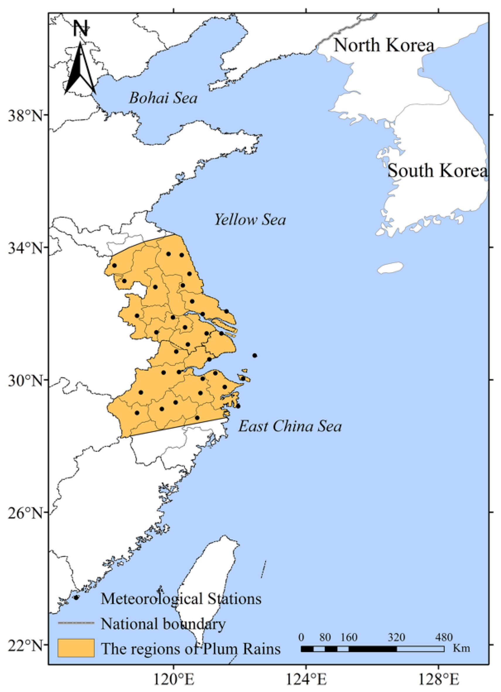
2.1. Study Area and Data

The study area includes most of the Jiangsu province, the Zhejiang province, and Shanghai, which are part of the middle and lower regions of the Yangtze River Delta. It is situated at a longitude of 116°18′ E–123°00’ E and latitude of 27°12′ N–35°20′ N. Its climate belongs to the sub-tropical monsoon climate, and the average temperature ranges from 2 to 4 °C in January and is above 28 °C in July. Annual precipitation is above 800 mm and the precipitation is mainly concentrated in the period of Plum Rains. The precipitation during the period of Plum Rains accounts for approximately 22.5% of the total annual precipitation. In addition, there are numerous lakes, and the recharge of the water mainly comes from atmospheric precipitation. It is well-known that this study area is one of the most developed areas in China with high levels of urbanization and industrialization. According to the Bulletin of the Sixth National Census, in 2010, the resident population had reached approximately 156 million [37].
Figure 1 shows the distribution of 33 meteorological stations, which are fairly uniformly distributed. The daily precipitation of 33 meteorological stations in the Yangtze River Delta from 1960 to 2012 comes from the China meteorological data network (http://data.cma.com). A uniform standard concerning the onset and termination of the Plum Rains was published on 12 May 2017 and implemented on 1 December 2017 (GB/T 33671-2017 Mei-yu Monitoring Indicators) [38]. From the first rainy day, the second day, the third day, etc., to the tenth day, if the ratio of the number of rainy days to the total number of days in the corresponding period is greater than or equal to 50%, the first rainy day is the beginning of Plum Rains. There is no new rainy beginning date after July 20. From the last rainy day of the rainy season, 2 days ago, 3 days ago, etc., to 10 days ago, if the number of rainy-day accounts for more than or equal to 50% of the number of rainy days in the corresponding period, the last rainy day is the termination of Plum Rains. If the number of rainy days accounts for less than 50% of the number of rainy days in the corresponding period, the last rainy day cannot be the termination of Plum Rains. It is necessary to push one day forward from the last rainy day of the rainy season, and then calculate whether the day is the termination of the Plum Rains, according to the conditions of the termination of the Plum Rains. If it is still not, this method is followed until the termination of the Plum Rains is found. For the abnormal rain season, the termination of Plum Rains occurs the day before the first non-rainy day after the rain period enters August. The termination of Plum Rains should appear before the start of the fall. For the sake of simplicity, it was assumed that the onset and termination of the Plum Rains were the same for each station, and the plum rainfall of each station for every year accumulated, according to the daily rainfall and the onset and termination of the Plum Rains, while the annual plum rainfall in the whole area was the average of the 33 stations. According to previous studies [25,26,27], we selected the PDO index, ENSO index, and EASM index to investigate the relationship between them and plum rainfall. The PDO index was obtained from http://research.jisao.washington.edu/pdo/PDO.latest. The ENSO data were gathered from http://research.jisao.washington.edu/datasets/globalsstenso. EASM index was defined as an area-averaged seasonally dynamic normalized seasonality index at 850 hPa within the East Asian monsoon domain (10°–40° N, 110°–140° E). The EASM index data were from the literature [39,40].

2.2. Methodology

To investigate the spatiotemporal variation of Plum Rains and its relation to EASM, ENSO, and PDO, we used an integrated approach combining the EEMD, EOF, and correlation analysis (Figure 2). We first showed the features of plum rainfall. Then, we used the EEMD method to decompose the plum rainfall into four intrinsic mode functions (i.e., IMF1, IMF2, IMF3, and IMF4) and a trend (RES). The influencing factors of the plum rainfall were also studied. We revealed the spatial pattern of the plum rainfall over the Yangtze River Delta during the period of 1960 to 2012. Lastly, we assessed the relationship between the EASM, ENSO, PDO, and plum rainfall on different time scales.

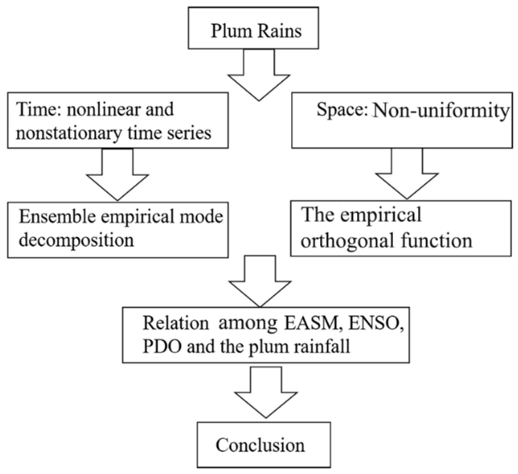
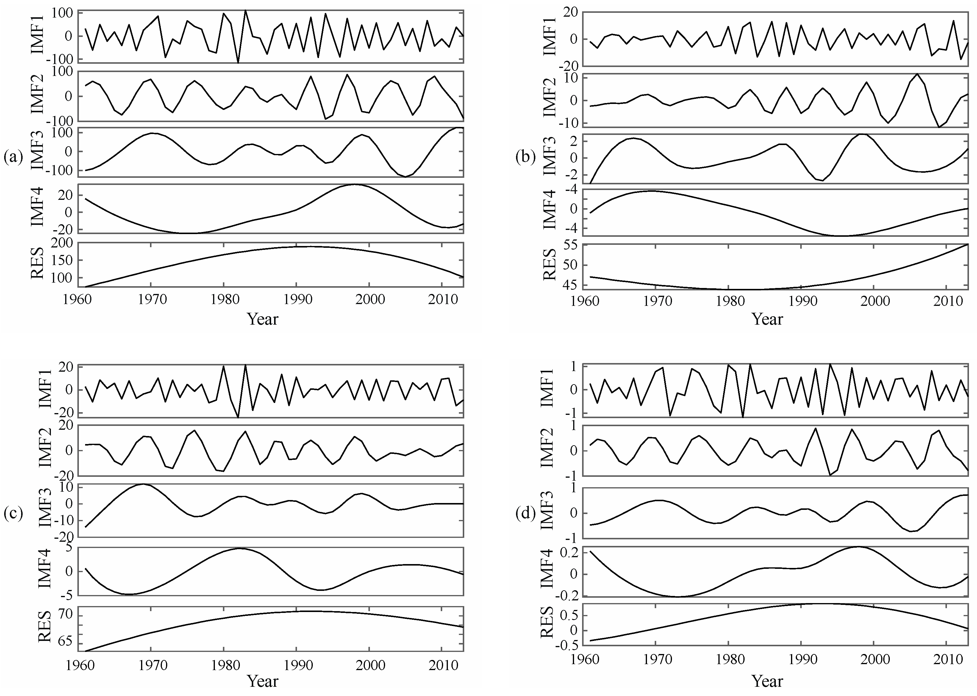
2.2.1. Ensemble Empirical Mode Decomposition

Ensemble empirical mode decomposition (EEMD) is utilized to analyze the nonlinear and periodic characteristics of the plum rainfall. It is based on empirical mode decomposition (EMD), and improvement of the EMD [41,42]. EMD is an effective method for dealing with the nonlinear and nonstationary time series problem, and it also has some advantages, such as self-adaptability, orthogonality, and completeness, etc. [43]. However, some defects still exist. One of the biggest defects is mode mixing, which makes a signal have different scales or frequencies in the same component or be decomposed into different components [44]. In order to solve this problem, Wu and Huang [45] proposed a new method, known as the EEMD, to better solve nonlinear problems. It can adaptively decompose the time-frequency, according to the local time variation features, and is completely free from the constraints of the Fourier transform so that it can obtain a high time-frequency resolution [41]. Therefore, we use the EEMD, which is the best decomposition method to extract the changes of various scales in the plum rainfall signal from the plum rainfall time series. The steps of the EEMD are as follows.
1. White noise with specified amplitude is added to the sequence of the original signal:
x i ( t ) = x ( t ) + n i ( t )
where x i ( t ) is the new signal after adding the white noise, x (t) is the original signal, and n i ( t ) is white noise.
2. By decomposing the signal, to which white noise has been added, using the EMD can result in IMF1 (the first Intrinsic Mode Function).
3. Adding the same white noise in the sequence that has separated out the IMF1 can result in IMF2 (the Second Intrinsic Mode Function) by using the EMD.
4. Repeating the above steps can result in different IMFs (the Intrinsic Mode Functions). In general, the standard deviation (SD) (generally be set as 0.2–0.3) between two consecutive results is used as a criterion for stopping the generation of IMFs [45]. When the SD reaches a certain threshold, the generation of IMFs is stopped. In this study, we set the threshold to 0.2 according to a previous study [18] and obtained four IMFs.
5. The IMFs obtained by each decomposition are collectively averaged so that the added white noises cancel each other out and can be used as the final decomposition result.
C j ( t ) = 1 N i = 1 N C i j ( t )
where C j ( t ) is the final jth IMF component, N is the number of white noise series, and C i j ( t ) denotes the jth IMF from the added white noise trial. From the above decomposition, the IMFs and trend term can be obtained at different scales. Next, the original signal is reconstructed.
x ( t ) = j = 1 n C j ( t ) + r n ( t )
After decomposing the original signal, each component should be tested for its significance. They can be tested by means of a set of white noise ensemble disturbance to obtain each IMF’s credibility [33]. The energy spectral density of the kth IMF is assumed to be the following.
E k = 1 N j = 1 N | I k ( j ) | 2
where N is the length of the IMF component and I k ( j ) denotes the kth IMF component. The white noise sequence is tested by the Monte Carlo method [44]. Then, a simple equation that relates the averaged energy density E ¯ k to the averaged period T ¯ k is obtained.
E ¯ k + ln { T ¯ k } = 0
In a figure of ln ( T ¯ k ) as the x-axis and ln ( E k ) as the y-axis, the relations between them can be expressed by a straight line whose slope is -1. The IMF component of the white noise series should, in theory, be distributed in a line. However, a little actual deviation is produced, so the confidence interval for the energy spectrum distribution of the white noise is presented as follows.
ln E ¯ k = ln { T ¯ k } a ± a 2 N e ln ( { T k } a 2 )
where a is the significance level. If the energy of the IMF is located above the confidence curve at a given significance level (e.g., a = 0.05), periodic oscillation has passed the significance test, and it can be assumed that the information at the selected confidence level contains physical meaning. Its corresponding oscillation period is the main oscillation period of the original sequence. However, if the energy of the IMFs falls outside the confidence curve at a given significance, it is considered to have not passed the significance test [42,46].

2.2.2. The Empirical Orthogonal Function

The spatiotemporal variation of plum rainfall has always been a hot issue. Different methods have been used to analyze it. The empirical orthogonal function (EOF), also known as the eigenvector analysis or principal component analysis (PCA), can describe the original variable field with fewer spatial distribution modalities and can cover most of the information in the original variable field [47,48]. It is helpful to analyze the spatiotemporal variations of the climate element field, and has become an important method for analyzing the characteristics of the variable field in climate research. The method was first proposed by the statistician Pearson in 1902, and then introduced into the analysis of climate problems by Lorenz (1956) [49]. Its analysis principle is as follows.
A climate variable field can be seen as a function of time and space. Suppose a climate variable field has m elements, and the time length is n, then the following is true.
X = [ x 11 x 12         x 1 n x 21 x 22         x 2 n                     x m 1           x m 2             x m n ]   ( i = 1 , 2 , , m ; j = 1 , 2 , , n )
where m is the spatial point, which can be the grid point or the observation point, n is the point in time, which is the number of samples, and xij represents the observation value of the point i at the point j. EOF expansion is employed to decompose the above equation into the sum of the product of the space function and the time function, which is shown below.
X = V T = k = 1 m v k j t k j ,   i = 1 , 2 , , m ; j = 1 , 2 , , n
where V represents the eigenvector matrix, and T represents the time coefficient matrix. According to the orthogonality, V and T satisfy the following conditions.
{ i = 1 m v i k v i l = 1       k = l i = 1 m v i k v i l = 0       k l
Next, according to Equation (10), the eigenvector, the eigenvalue, and the time coefficient matrix T can be obtained. The eigenvalues are arranged in descending order ( λ 1 λ 2 λ m 0 ), and the variance contribution rate of each eigenvector (Rk) can be obtained by the following formula.
R k = λ k / i = 1 m λ i , k = 1 , 2 ,   , p ( p < m )

3. Results

3.1. The Time Variation of Plum Rainfall

As seen in Figure 3, the plum rainfall in the Yangtze River Delta over the period of 1960 to 2012 presented an increasing and then decreasing trend. A turning point appeared in the 1990s. Before that, the plum rainfall showed an increasing trend, and after that, the plum rainfall showed a decreasing trend. The plum rainfall was higher in the years of 1969, 1982, 1996, and 1998, and lower in the years of 1965, 1971, 1978, and 2006. In addition, it can be seen that the plum rainfall was not linear, but shows a nonlinear variation trend (see Figure 3). Therefore, a nonlinear method should be used to analyze the nonlinear and non-stationary variations of plum rainfall.
As we know, the formation process of Plum Rains is a complex nonlinear system, which is influenced by natural factors and human activities [50], and has many uncertainties, such as ambiguity and randomness. Simple statistical analysis, such as linear regression analysis and correlation analysis, can only describe linear time series, and cannot reveal the regularity of nonlinear and non-stationary time series. Studies have shown that EEMD is an improvement of EMD [41] and exhibits a stronger local performance than wavelet analysis [51,52]. Therefore, we used the EEMD to extract the variations of various scales in terms of the plum rainfall, the onset of Plum Rains, the termination of Plum Rains, and the daily intensity of the plum rainfall signal from their original time series to reveal the oscillating mode structure characteristics at different time scales and explore evolution characteristics of these different scale oscillations.
Figure 4 shows the EEMD results of the four-time series. There were four IMFs (IMF1-4) and one trend component (RES) of plum rainfall, the onset of Plum Rains, the termination of Plum Rains, and the daily intensity of plum rainfall, respectively. The components represent the oscillation characteristics from high to low frequency of the original sequence on different scales and all have a specific physical meaning, while the tendency term represents the variation characteristic as a whole [42]. As shown in Figure 4a, plum rainfall displayed three-year (IMF1) and six-year (IMF 2) periodic fluctuation at the inter-annual scale and 14-year (IMF3) and 33-year (IMF4) periodic variation at the inter-decadal scale. In other words, there may be some dry Plum Rains seasons after a few wet Plum Rains seasons. The result is useful for local governments and farmers to predict and mitigate the effects of droughts and floods. The trend term reflects the variations of plum rainfall, which increased gradually before the 1990s and then decreased gradually. However, previous studies showed that the plum rainfall in the YRD presented an increasing trend in past decades [28,53]. The difference is that they analyzed the variations of plum rainfall from the perspective of the linear trend, but we used the nonlinear method. It can be seen that previous studies did not reflect details of the variations of plum rainfall, which illustrates that the EEMD is an optimal method for dealing with nonlinear problems. In addition, we produced EEMD results for the onset and termination of Plum Rains and the daily intensity of plum rainfall (Figure 4b–d). The onset of Plum Rains exhibited three-year (IMF1) and six-year (IMF2) periodic fluctuation at the inter-annual scale and 14-year (IMF3) and 49-year (IMF4) periodic variation at the inter-decadal scale. The termination of Plum Rains displayed three-year (IMF1), six-year (IMF2), and nine-year (IMF3) periodic fluctuation at the inter-annual scale and 24-year (IMF4) periodic variation at the inter-decadal scale. The daily intensity of plum rainfall showed three-year (IMF1) and five-year (IMF2) periodic fluctuation at the inter-annual scale and 27-year (IMF3) and 51-year (IMF4) periodic variation at the inter-decadal scale. It can be seen that the plum rainfall had similar cycles with the onset and termination of Plum Rains and the daily intensity of plum rainfall on the inter-annual scale. Their trend terms were the same as those for plum rainfall, which means that the variation of plum rainfall is mainly affected by the onset and termination of Plum Rains and the daily intensity of plum rainfall, and the result was consistent with previous studies [13,15]. However, unlike previous studies, the effect of the onset and termination of Plum Rains and the daily intensity of plum rainfall on the inter-annual scale is greater than on the inter-decadal scale.
It is necessary to conduct significant tests in order to determine whether each component is a result of simple noise, or a signal that has physical meaning. In Figure 5, the horizontal coordinate represents periodic data and the vertical coordinate represents the energy spectrum density with four confidence levels, which are 80%, 90%, 95%, and 99%. It indicates that the IMF passes the significance test and has many physical meanings if it falls above the confidence level. Otherwise, IMF contains pure white noise. In other words, more or less physical meaning actually means strong or weak oscillations within a certain range. IMF1, IMF2, and IMF3 of plum rainfall fell above the confidence level of 90% and IMF4 of plum rainfall fell between the confidence level of 80% and 90%. IMF1, IMF2, and IMF3 comprised a more definite physical meaning but not white noise, and IMF4 contained less physical meaning. IMF1 and IMF4 of the onset of Plum Rains fell above the confidence level of 95%, while IMF2 and IMF3 of the onset of Plum Rains fell below the confidence level of 90%. IMF1, IMF2, and IMF3 of the termination of Plum Rains fell above the confidence level of 90% while IMF4 fell below the confidence level of 90%. IMF1, IMF2, and IMF3 of the intensity of plum rainfall fell above the confidence level of 90%, while IMF4 fell below the confidence level of 80%.
Each component’s variation contribution rate was calculated to compare each component and the inherent oscillation characteristics in the original sequence. Table 1 presents the results of the variance contribution rates of the EEMD for the plum rainfall, the onset and termination of Plum Rains, and the intensity of plum rainfall. Significant IMFs are shown in bold in Table 1. The changes of each component are the common consequences of the internal dynamic process and the external force factors of the atmosphere. We can note that the largest variance contribution rate was IMF1, followed by IMF2, RES, IMF3, and IMF4 for plum rainfall and the intensity of plum rainfall. The largest variance contribution rate was IMF1, followed by IMF2, RES, IMF4, and IMF3 for the onset of plum rainfall. Additionality, the largest variance contribution rate was IMF1, followed by IMF2, IMF3, IMF4, and RES for the termination of Plum Rains. Although the variance contribution rate of each component is different for plum rainfall, the onset and termination of Plum Rains, and the intensity of plum rainfall, their common point is that the variance contribution rate on the inter-annual scale is greater than the inter-decadal scale.

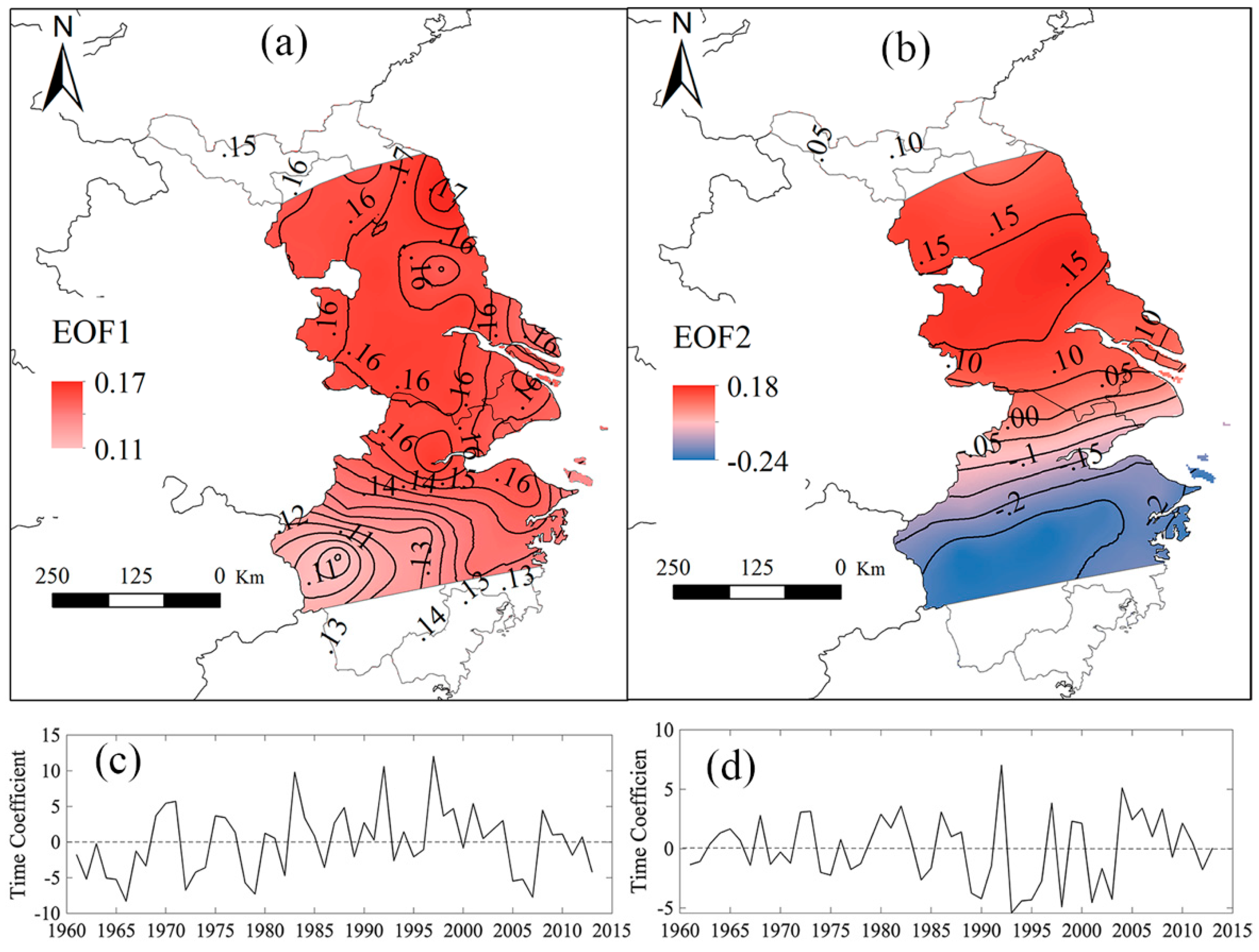
3.2. Spatial Pattern of Plum Rainfall

In order to explore the spatial pattern variation of plum rainfall during the period of 1960 to 2012, the EOF method is used. First, we obtained six principal components and they passed the North test [54]. The main results are shown in Table 2. It can be seen that the variance contribution rate of the first principal component was the largest, which was 50.48. The variance contribution rate of the second principal component decreased rapidly, and the variance contribution rate of the third and other principal components was small. The variance contribution rate of the first two principal components reached 70%. Therefore, we only gave the eigenvector fields corresponding to the first two principal components.
Figure 6a shows the first eigenvector field and all values are positive. This means that the increase or decrease of plum rainfall is consistent in the entire region. That is, if the value is positive, the plum rainfall in the entire study region will increase, and, if the value is negative, the plum rainfall in the entire study region will decrease, so it can be said that it is affected by the large-scale atmospheric circulation. The high value was mainly distributed in the northern part of the region, which indicates that it was the region with the highest variability of plum rainfall and it was the most sensitive region of drought and flood. The low value was mainly distributed in the southwest part of this region, which indicates that it was the region with a low variability of plum rainfall. These results illustrate that the plum rainfall is also affected by local factors. The related temporal coefficient curve (Figure 6c) mostly depicts variations on 4-year to 6-year time scales, which are similar to the EEMD result. Results of EOF and EEMD can be verified with each other. The results of EOF can prove the rationality of EEMD, and the results of EEMD can also prove the rationality of EOF. In addition, the time coefficient in 1996 was the largest and positive, which indicates that the plum rainfall in this year was the highest. This was a typical rainy year, followed by 1982 and 1991. The time coefficients in 1965, 1971, 1978, and 2006 were the smallest and negative, which indicates that they were the typical years of little plum rainfall.
It can be seen from Figure 6b that there was a large difference between the first eigenvector field and the second eigenvector field. From Figure 6b, we can see that the positive values were distributed in the north of the region, while the negative values were distributed in the south of the region. This indicates that the plum rainfall showed an out-of-phase pattern of about 30° N between the north and south area. This means that there is less plum rainfall in the south when there is more plum rainfall in the north and there is more plum rainfall in the south when there is less plum rainfall in the north. The reason for this phenomenon is mainly due to the different location of the Plum Rains’ belt every year. When the Plum Rains’ belt stays in the south of the Yangtze River for a long time, there is a lot of plum rainfall in the south. When the Plum Rains’ belt stays in the Jiang-Huai area for a long time, there is more plum rainfall in the north. Figure 6d shows that the time coefficient in 1991 was the largest and positive, which meant that it was the typical year with more plum rainfall in the north and less plum rainfall in the south, which was followed by 1996 and 2003. The time coefficient in 1992 was the smallest and negative, which meant that it was the typical year with more plum rainfall in the south and less plum rainfall in the north.

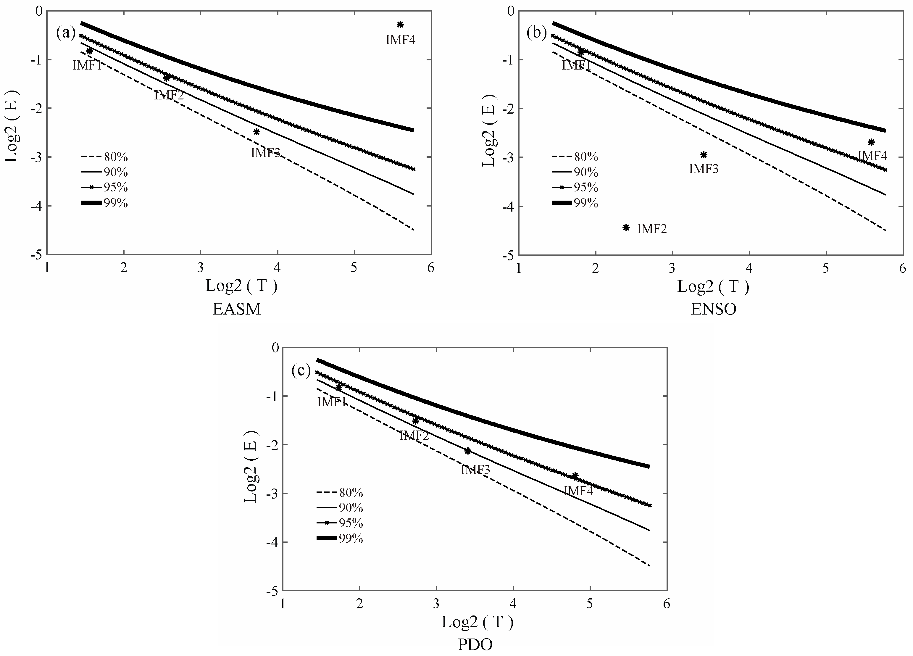
3.3. The Relation among EASM, ENSO, PDO, and Plum Rainfall

The variations of plum rainfall are complex and have a direct relationship with atmospheric circulation. Previous studies have analyzed the influencing factors of plum rainfall on the whole [55,56,57], while ignoring the relationship between them in detail. Therefore, we have tried to explore the impact of EASM, ENSO, and PDO on plum rainfall from multi-time scales. Table 3 shows the EEMD results for plum rainfall, EASM, ENSO, and PDO. There were four IMF components for each index and they all had similar periods on both the inter-annual scale and the inter-decadal scale. This means that there is a relationship between EASM, ENSO, PDO, and plum rainfall, but the specific relationship between them at different time scales still needs to be discussed. However, the fourth IMF component of plum rainfall was different from EASM and ENSO, and the period of EASM and ENSO was longer than the period of plum rainfall. The period of PDO was shorter than the period of plum rainfall.
We performed significance tests to determine whether each component of EASM, ENSO, and PDO is a physically meaningful signal, or the result of simple noise. In Figure 7, IMF2 and IMF4 of EASM fell above the confidence level of 90%, while IMF1 and IMF3 fell below the confidence level of 90%, which meant that IMF2 and IMF4 contained more physical meaning and IMF1 and IMF3 contained more white noise. IMF1 and IMF4 of ENSO fell above the confidence level of 90%, while IMF2 and IMF3 of ENSO fell below the confidence level of 80%, which meant that IMF1 and IMF4 contained more physical meaning while IMF2 and IMF3 contained less physical meaning. IMF1, IMF2, and IMF4 of PDO fell above the confidence level of 90% and IMF3 of PDO fell between the confidence level of 80% and 90%. This meant that IMF1, IMF2, and IMF4 comprised a more definite physical meaning, and IMF3 contained a less physical meaning. Significant IMFs are shown in bold in Table 3.
Then, the correlation analysis was applied in order to understand the relation between plum rainfall and EASM, ENSO, and PDO more clearly. We first obtained the components of plum rainfall, EASM, ENSO, and PDO on four-time scales, and then calculated the correlation of plum rainfall and EASM, ENSO, and PDO on each time scale, respectively. The results are shown in Table 4. Significant correlations are shown in bold. On the inter-annual scale, IMF2 of plum rainfall had a negative and significant correlation with IMF2 of EASM. The result was similar to the results of some previous studies [58,59,60], but the difference was that they did not discuss the relation between plum rainfall and EASM on multi-time scales. Our result indicated that EASM had a significant impact on plum rainfall on an interannual scale rather than on the entire time scale. The correlation between IMF1 of plum rainfall and IMF1 of ENSO was positive and significant, which indicated that ENSO had a significant influence on plum rainfall in a three-year periodic fluctuation. On the inter-decadal scale, although all components of plum rainfall had some association with the components of EASM and ENSO, neither of them passed the significance test. It can be said that EASM and ENSO were not the main influencing factors of plum rainfall on the inter-decadal scale. The correlation between IMF4 of plum rainfall and IMF4 of PDO was positive, but the correlation between IMF3 of plum rainfall and IMF3 of PDO was negative. From the above results, we know that IMF4 of plum rainfall and IMF3 of PDO were not significant. Therefore, we cannot say that PDO was the main influencing factor of plum rainfall on the inter-decadal scale during the period of 1960 to 2012, and the relationship between plum rainfall and PDO needs to be further confirmed. This study gives a simple correlation between them. In summary, ENSO and EASM were the main influencing factors in the three-year and six-year periods, respectively, and the main influencing factors on the inter-decadal scale remains to be further studied. This means that on the time scale of three years, the plum rainfall is mainly affected by ENSO. On the time scale of six years, the plum rainfall is mainly affected by EASM. Therefore, it is necessary to separate the diverse time scales when forecast and climate changes are studied.

4. Discussion

This study first investigated the multi-time scale temporal variation of plum rainfall in the YRD by using the EEMD method and then analyzed the spatial pattern of plum rainfall by using the EOF method. Lastly, we showed the relationship between plum rainfall and EASM, ENSO, and PDO. We found that, in the past 53 years, plum rainfall has three-year and six-year cycles on the inter-annual scale and 14-year and 33-year cycles on the inter-decadal scale. The plum rainfall variability was dominated by the inter-annual scale. In addition, the first EOF showed in-phase changes of plum rainfall across the whole study region and the second EOF showed an out-of-phase plum rainfall pattern between the north and south areas of about 30° N. The changes of plum rainfall were affected by ENSO and EASM in the three-year and six-year periods, respectively. Whether PDO was the main influencing factor on the inter-decadal scale remains to be further studied.
Few studies have analyzed variations of the Plum Rains from multi-time scales, and most of them have used the wavelet analysis method and rarely used the EEMD method [17,26]. It has been proven that the EEMD method is superior to the wavelet analysis method [51,52]. Our study used the EEMD method to analyze the multi-time-scale variations of plum rainfall, the multi-time-scale variations of the onset of Plum Rains, the termination of Plum Rains, and the intensity of plum rainfall, which can, more accurately, identify their variation periods. We found that plum rainfall had three-year and six-year cycles on the inter-annual scale and 14-year and 33-year cycles on the inter-decadal scale. IMF1, IMF2, and IMF3 all passed the significance test. However, IMF4 of plum rainfall was not significant, even though it accounted for a large fraction of the variance, which meant that it was not possible to say whether there was a 33-year cycle in plum rainfall. Wei and Xie [17] used the wavelet analysis method to analyze the multi-time scales variations of plum rainfall, and they found that the plum rainfall had cycles of 2 to 3 years, 6 to 7 years, 23 to 24 years, and 36 to 37 years in the entire Yangtze-Huaihe River region. Zhang et al. [26] pointed out that plum rainfall existed for about a three-year to six-year short cycle and 11-year and 20-year-long cycles by using the wavelet analysis method in the entire Yangtze-Huaihe River region. Bai et al. [18] showed that the plum rainfall had three-year, six-year, 13-year, and 24-year cycles in the Middle-Lower Reaches of the Yangtze River. Compared with previous studies, we found that plum rainfall has similar variations on the interannual scale, but the variation on the interdecadal scale is very large in different regions. This is mainly due to the fact that, on the interdecadal scale, the influence of various factors on plum rainfall in different regions is more complicated, which illustrates the importance of regional differences. In addition, we also found that the onset of Plum Rains had three-year, six-year, 14-year, and 49-year cycles, but six-year and 14-year cycles were not significant, even though they accounted for a large fraction of the variance, which meant that the onset of Plum Rains only had significant three-year and 49-year cycles. Similarly, the termination of Plum Rains had significant three-year, six-year, and nine-year cycles (IMF4 is not significant), and the intensity of plum rainfall had significant three-year, five-year, and 27-year cycles (IMF4 is not significant). It can be seen that the onset of Plum Rains, the termination of Plum Rains, and the intensity of plum rainfall had similar cycles with plum rainfall, which reveals their relationship with plum rainfall on multi-time scales. Previous studies have analyzed the relationship between the onset of Plum Rains, the termination of Plum Rains, and the intensity of plum rainfall as well as plum rainfall from the perspective of the linear trend [61,62]. Prior studies did not discuss it from multi-time scales. We can see from the above results that variations of the onset of Plum Rains, the termination of Plum Rains, and the intensity of plum rainfall are nonlinear, so it is necessary to explore their relationship at multi-time scales.
As far as the spatial pattern of plum rainfall is concerned, Chen and Li [63] analyzed the spatial pattern in the Yangtze-Huaihe River region during the period of 1960 to 2012 using the EOF method. They found that there were four modes, the first of which was characterized by the simultaneous increase or decrease of the plum rainfall in the whole region, and the second of which was characterized by more plum rainfall in the north (south) and less plum rainfall in the south (north). Our result was consistent with this. However, the difference was that there were two other local spatial patterns in their study. It may be because our study region is small, which cannot recognize the smaller spatial pattern. Li et al. [64] found a different spatial pattern of plum rainfall. They pointed out that the first mode of plum rainfall showed a spatial pattern of more (less) plum rainfall in the south and less (more) plum rainfall in the north, and the second mode showed a spatial pattern of more (less) plum rainfall in the middle and less (more) plum rainfall on both sides, which was different from our results. This is mainly due to regional differences and differences in research times. Therefore, it can be seen that, although the Plum Rains season is formed by some common factors, it does not mean that the plum rainfall has completely consistent variation. Therefore, it is necessary to study the spatiotemporal variations of plum rainfall in different sub-regions. The sub-regional analysis of the spatiotemporal variations of the plum rainfall is meaningful to formulate agricultural and industrial development policies, according to local conditions. In addition, it is worth mentioning that our study only analyzes an average state for a period of 53 years, and does not discuss the spatial pattern of plum rainfall in different time periods, which needs to be further studied in the future.
In addition, we also assessed the relationship between ENSO, EASM, PDO, and plum rainfall on multi-time scales. Many studies have explored the effects of atmospheric circulation on Plum Rains from statistical methods or physics-based methods [58,59,60]. The difference between our study and previous studies was that previous studies studied the relationship between plum rainfall and EASM, ENSO, and PDO from the average state, and we explored the relationship between ENSO, EASM, PDO, and plum rainfall from multi-time scales. It was also found that ENSO and EASM are the main influencing factors in the three-year and six-year periods, respectively. In addition, the correlation between IMF3 of plum rainfall and IMF3 of PDO and the correlation between IMF4 of plum rainfall and IMF4 of PDO were significant. However, the IMF4 of plum rainfall and IMF3 of PDO were not significant. Therefore, we cannot say that PDO was the main influencing factor of plum rainfall during the period of 1960 to 2012. Jiang and Gao [61] pointed out that the amount of plum rainfall would increase when PDO was in a positive phase compared to a normal year. In this study, we did not get the same results, and the difference is that Jiang and Gao did not study the relationship between plum rainfall and PDO on multi-time scales, as we did. Due to the short observational record in this study, we will study the relationship between plum rainfall and PDO at multi-time scales for longer observational records. Whether PDO is the main influencing factor of plum rainfall on the inter-decadal scale remains to be further studied. This study builds on previous ones by exploring different aspects of the Plum Rains onset and withdrawal variability. However, this study has only analyzed the relationship between ENSO, EASM, PDO, and plum rainfall at multi-time scales by using statistical methods and has not explained the reasons for the different relationships at different time scales in terms of the physical mechanism, which requires further research.

5. Conclusions

The spatiotemporal variation of plum rainfall and its relation to EASM, ENSO, and PDO was investigated using a dataset from 33 meteorological stations on the onset and termination of Plum Rains as well as daily precipitation during the period of 1960 to 2012. An integrated approach combining the EEMD, EOF, and correlation analysis was employed. The main conclusions are reproduced below.
(1) By analyzing the time series at the onset and termination of Plum Rains, the daily intensity of plum rainfall, and plum rainfall, we found that, in the past 53 years, the plum rainfall had three-year and six-year cycles on the inter-annual scale and 14-year and 33-year cycles on the inter-decadal scale. Additionally, it showed a trend of increasing first and then decreasing. In addition, the onset of Plum Rains, the termination of Plum Rains, and the daily intensity of plum rainfall had similar cycles and trends to plum rainfall. Furthermore, the effect of the onset and termination of Plum Rains and the daily intensity of plum rainfall on plum rainfall on the inter-annual scale was greater than on the inter-decadal scale.
(2) There are two obvious characteristics of the spatial pattern of plum rainfall. The first EOF was characterized by in-phase changes across the whole study region. The second EOF showed an out-of-phase plum rainfall pattern of about 30° N between the areas north and south. It is necessary to analyze the spatiotemporal variations of plum rainfall in different sub-regions.
(3) The changes in plum rainfall were affected by different factors on different time scales. The difference was that ENSO and EASM were the main influencing factors in the three-year and six-year periods, respectively, and whether PDO was the main influencing factor on the inter-decadal scale remains to be further studied. Studying the influence of atmospheric circulation on plum rainfall at multi-time scales can give us a deeper understanding of it.

Author Contributions

N.Z. designed, carried out the analysis, and wrote the manuscript. J.X. revised the paper and refined the results, conclusion, and abstract. K.L. and C.Z. discussed the results. Y.L. edited the figures. All authors approved the manuscript.

Funding

This research received no external funding.

Acknowledgments

The authors are grateful to the Resource and Environmental Science Data Center (http://www.resdc.cn) of the Chinese Academy of Sciences and the China Meteorological Data Sharing Service System (http://cdc.cma.gov.cn/) for providing data. The authors appreciate the insightful comments of anonymous reviewers.

Conflicts of Interest

The authors declare no conflict of interest.

References

  1. Ninomiya, K. Characteristics of Baiu front as a predominant subtropical front in the summer Northern Hemisphere. J. Meteor. Soc. Jpn. 1984, 62, 880–894. [Google Scholar] [CrossRef]
  2. Akiyama, T. The large-scale aspects of the characteristic features of the Baiu front. Meteor. Geophys. 1973, 24, 157–188. [Google Scholar] [CrossRef]
  3. Kodama, Y.-M. Large-scale common features of subtropical precipitation zones (the Baiu frontal zone, the SPCZ, and the SACZ). Part I: Characteristics of subtropical frontal zones. J. Meteorol. Soc. Jpn. 1992, 70, 813–836. [Google Scholar] [CrossRef]
  4. Sampe, T.; Xie, S.P. Large-scale dynamics of the Meiyu-Baiu rainband: Environmental forcing by the westerly jet. J. Climatol. 2010, 23, 113–134. [Google Scholar] [CrossRef]
  5. Huang, Z.; Xu, H.; Hu, J. Review and Discussion on the Plum Rain Research in China. Meteorol. Environ. Res. 2011, 2, 25–29. [Google Scholar] [CrossRef]
  6. You, C.H.; Lee, D.I.; Jang, S.M.; Jang, M.; Uyeda, H.; Shinoda, T.; Kobayashi, F. Characteristics of rainfall systems accompanied with Changma front at Chujado in Korea. Asia-Pac. J. Atmos. Sci. 2010, 46, 41–51. [Google Scholar] [CrossRef]
  7. Zhu, K.Z. The southeast summer monsoon and precipitation of China. J. Geogr. Sci. 1934, 1, 1–27. [Google Scholar]
  8. Tu, C.W. Chinese air mass properties. Q. J. R. Meteorol. Soc. 1939, 65, 33–51. [Google Scholar] [CrossRef]
  9. Lu, A. Precipitation in the South Chinese-Tibetan Borderland. Geogr. Rev. 1947, 37, 88–93. [Google Scholar] [CrossRef]
  10. Kang, I.S.; Ho, C.H.; Lim, Y.K. Principle modes of climatological seasonal and intraseasonal variations of the Asian summer monsoon. Mon. Weather Rev. 1999, 127, 322–340. [Google Scholar] [CrossRef]
  11. Zhou, H. Study on the mesoscale structure of the heavy rainfall on Meiyu front with dual-Doppler RADAR. Atmos. Res. 2009, 93, 335–357. [Google Scholar] [CrossRef]
  12. Huang, D.Q.; Qian, Y.F.; Zhu, J. The heterogeneity of Meiyu rainfall over Yangtze-Huaihe River vally and its relationship with oceanic surface heating and intraseasonal variability. Theor. Appl. Climatol. 2012, 108, 601–611. [Google Scholar] [CrossRef]
  13. Gao, Q.; Sun, Y.; You, Q. The northward shift of Meiyu rain belt and its possible association with rainfall intensity changes and the Pacific-Japan pattern. Dyn. Atmos. Ocean. 2016, 76, 52–62. [Google Scholar] [CrossRef]
  14. Matsumoto, J. Heavy rainfall over East Asia. Int. J. Climatol. 1988, 9, 407–423. [Google Scholar] [CrossRef]
  15. Lee, D.K.; Kim, Y.A. Variability of the East Asian summer monsoon during the period of 1980–1989. J. Korean Meteorol. Soc. 1992, 28, 315–331. [Google Scholar]
  16. Chen, C. Investigation of a heavy rainfall event over southwestern Taiwan associated with a sub-synoptic cyclone during the 2003 Mei-Yu season. Atmos. Res. 2010, 95, 235–254. [Google Scholar] [CrossRef]
  17. Wei, F.Y.; Xie, Y. Interannual and interdecadal oscillations of Meiyu over the middle-lower reaches of the Changjiang River for 1885–2000. J. Appl. Meteorol. Climtol. 2005, 16, 492–499. [Google Scholar] [CrossRef]
  18. Bai, L.; Chen, Z.S.; Zhao, B.F. Application of Ensemble Empirical Mode Decomposition Method in Multiscale analysis of Meiyu in Middle-Lower Reaches of Yangtze River. Resour. Environ. Yangtze Basin 2015, 24, 482–488. [Google Scholar] [CrossRef]
  19. Jiang, J.Y.; Ni, Y.Q. Diagnostic study on the structural characteristics of a typical Meiyu front system and its maintenance mechanism. Adv. Atmos. Sci. 2004, 21, 802–813. [Google Scholar] [CrossRef]
  20. Shinoda, T.; Uyeda, H.; Yoshimura, K. Structure of moist layer and sources of water over the southern region far from the Meiyu/Baiu front. J. Meteorol. Soc. Jpn. 2005, 83, 137–152. [Google Scholar] [CrossRef]
  21. Zhou, X.J.; Zha, P.; Liu, G.; Zhou, T.J. Characteristics of decadal-centennial-scale changes in East Asian summer monsoon circulation and precipitation during the medieval warm period and little ice age and in the present day. Chin. Sci. Bull. 2011, 56, 3003–3011. [Google Scholar] [CrossRef]
  22. Liu, D.N.; He, J.H.; Yao, Y.H.; Qi, L. Characteristics and Evolution of Atmospheric Circulation Patterns during Meiyu over the Jianghuai valley. Asia-Pac. J. Atmos. Sci. 2012, 48, 145–152. [Google Scholar] [CrossRef]
  23. Wu, Y.T.; Shaw, T.A. The Impact of the Asian Summer Monsoon Circulation on the Tropopause. J. Climatol. 2016, 8, 8689–8701. [Google Scholar] [CrossRef]
  24. Yu, J.; Huang, X.; Yu, Y.; Guo, X.; Dong, B.; Lu, T.; Wang, H. Analysis on the new index of plum rains intensity and its spatio-temporal characteristics: A case study on the reaches of the region along Huaihe River in Anhui Province. Sci. Agric. Sin. 2009, 42, 1325–1330. [Google Scholar]
  25. Chen, S.J.; Kuo, Y.W.; Wang, W.; Tao, Z.Y.; Cui, B. A Modeling Case Study of Heavy Rainstorms along the Mei-Yu Front. Mon. Weather Rev. 1998, 126, 2330. [Google Scholar] [CrossRef]
  26. Zhang, Y.; Zhai, P.; Qian, Y. Variations of Meiyu indicators in the Yangtze-Huaihe River basin during 1954–2003. Acta Meteorol. Sin. 2005, 19, 479–484. [Google Scholar]
  27. Zhu, X.; Wu, Z.; He, J. Anomalous Meiyu onset averaged over the Yangtze River valley. Theor. Appl. Climatol. 2008, 94, 81–95. [Google Scholar] [CrossRef]
  28. Zhu, J.; Huang, D.Q.; Zhang, Y.C.; Huang, A.N.; Kuang, X.Y.; Huang, Y. Decadal changes of Meiyu rainfall around 1991 and its relationship with two types of ENSO. J. Geophys Res. Atmos. 2013, 118, 9766–9777. [Google Scholar] [CrossRef]
  29. Xue, F.; Liu, C.Z. The influence of moderate ENSO on summer rainfall in eastern China and its comparison with strong ENSO. Chin. Sci. Bull. 2008, 53, 791–800. [Google Scholar] [CrossRef]
  30. Wang, H.; Yao, J.Q.; Shi, C.H.; Chen, B.M. The relationship between Meiyu and the intensity of East Asian Summer Monsoon. Plateau Meteorol. 2008, 27, 109–117. [Google Scholar]
  31. Zhang, N.; Gao, Z.; Wang, X.; Chen, Y. Modeling the impact of urbanization on the local and regional climate in Yangtze River Delta, China. Theor. Appl. Climatol. 2010, 102, 331–342. [Google Scholar] [CrossRef]
  32. Feng, Z.; Jin, M.; Zhang, F.; Huang, Y. Effects of ground-level ozone (O3) pollution on the yields of rice and winter wheat in the Yangtze River Delta. J. Environ. Sci. China 2003, 15, 360–362. [Google Scholar] [CrossRef]
  33. Zhang, Q.; Gemmer, M.; Chen, J. Climate changes and flood/drought risk in the Yangtze Delta, China, during the past millennium. Quat. Int. 2008, 176, 62–69. [Google Scholar] [CrossRef]
  34. Wang, Y.; Xu, Y.; Lei, C.; Li, G.; Han, L.; Song, S.; Yang, L.; Deng, X. Spatio-temporal characteristics of precipitation and dryness/wetness in Yangtze River Delta, eastern China, during 1960–2012. Atmos. Res. 2016, 172, 196–205. [Google Scholar] [CrossRef]
  35. Chen, W.; Cutter, S.L.; Emrivh, C.T.; Shi, P. Measuring social vulnerability to natural hazards in the Yangtze River Delta region, China. Int. J. Disaster Risk Sci. 2013, 4, 169–181. [Google Scholar] [CrossRef]
  36. Zhu, N.; Xu, J.; Li, W.; Li, K.; Zhou, C. A Comprehensive Approach to Assess the Hydrological Drought of Inland River Basin in Northwest China. Atmosphere 2018, 9, 370. [Google Scholar] [CrossRef]
  37. The Sixth Census Commission. The Main Data Bulletin for the Sixth National Census in 2010 (No. 1); Sixth Census Commission: Beijing, China, 2010. [Google Scholar]
  38. General Administration of Quality Supervision, Inspection and Quarantine of the People’s Republic of China and China National Standardization Management Committee. Mei-Yu Monitoring Indicators; Standards Press of China: Beijing, China, 2017. [Google Scholar]
  39. Li, J.P.; Zeng, Q.C. A new monsoon index and the geographical distribution of the global monsoons. Adv. Atmos. Sci. 2003, 20, 299–302. [Google Scholar] [CrossRef]
  40. Li, J.P.; Zeng, Q.C. A unified monsoon index. Geophys. Res. Lett. 2002, 29, 1274. [Google Scholar] [CrossRef]
  41. Chu, W.; Qiu, S.; Xu, J. Temperature change of Shanghai and its response to global warming and urbanization. Atmosphere 2016, 7, 114. [Google Scholar] [CrossRef]
  42. Xu, J.; Chen, Y.; Bai, L.; Xu, Y. A hybrid model to simulate the annual runoff of the Kaidu River in northwest China. Hydrol. Earth Syst. Sci. 2016, 20, 1447–1457. [Google Scholar] [CrossRef]
  43. Bai, L.; Xu, J.; Chen, Z.; Li, W.; Liu, Z.; Zhao, B.; Wang, Z. The regional features of temperature variation trends over Xinjiang in China by the ensemble empirical mode decomposition method. Int. J. Climatol. 2015, 35, 3229–3237. [Google Scholar] [CrossRef]
  44. Wu, Z.H.; Huang, N.E. Ensemble empirical mode decomposition: A noise-assisted data analysis method. Adv. Adap. Data Anal. 2009, 1, 1–41. [Google Scholar] [CrossRef]
  45. Huang, N.E.; Shen, Z.; Long, S.R.; Wu, M.C.; Shih, H.H.; Zheng, Q.; Yen, N.C.; Tung, C.C.; Liu, H.H. The empirical mode decomposition and the Hilbert spectrum for nonlinear and non-stationary time series analysis. Proceedings of the Royal Society of London. Series A: Mathematical. Phys. Eng. Sci. 1998, 454, 903–995. [Google Scholar] [CrossRef]
  46. Zhu, N.; Xu, J.; Wang, C.; Chen, Z.; Luo, Y. Modeling the multiple time scale response of hydrological drought to climate change in the data-scarce inland river basin of Northwest China. Arab. J. Geosci. 2019, 12, 225. [Google Scholar] [CrossRef]
  47. Xoplaki, E.; Luterbacher, J.; Burkard, R.; Patrikas, I.; Maheras, P. Connection between the large-scale 500 hPa geopotential height fields and precipitation over Greece during wintertime. Climatol. Res. 2000, 14, 129–146. [Google Scholar] [CrossRef]
  48. Kikuchi, K.; Wang, B. Diurnal precipitation regimes in the global tropics. J. Climate 2008, 21, 2680–2696. [Google Scholar] [CrossRef]
  49. Lorenz, E.N. Empirical orthogonal functions and statistical weather prediction. In Technical Report; Statistical Forecast Project Report 1; Dept. of Meteor. MIT: Cambridge, MA, USA, 1956; p. 49. [Google Scholar]
  50. Fu, C. Potential impacts of human-induced land cover change on East Asia monsoon. Glob. Planet. Chang. 2003, 37, 219–229. [Google Scholar] [CrossRef]
  51. Ayenu-Prah, A.Y.; Attoh-Okine, N.O. Comparative study of Hilbert-Huang transform, Fourier transform and wavelet transform in pavement profile analysis. Veh. Syst. Dyn. 2009, 47, 437–456. [Google Scholar] [CrossRef]
  52. Alexandrov, T. A method of trend extraction using singular spectrum analysis. Rev. Stat. J. 2009, 7, 1–22. [Google Scholar]
  53. He, J.H.; Wu, Z.W.; Jiang, Z.H.; Miao, C.S.; Han, G.R. “Climate effect” of the northeast cold vortex and its influences on Meiyu. Chin. Sci. Bull. 2007, 52, 671–679. [Google Scholar] [CrossRef]
  54. North, G.R.; Bell, T.L.; Cahalan, R.F. Sampling errors in the estimation of the empirical orthogonal functions. Mon. Weather Rev. 1982, 110, 699–706. [Google Scholar] [CrossRef]
  55. Hao, Z.; Zheng, J.; Ge, Q. Variations in the summer monsoon rainbands across eastern China over the past 300 years. Adv. Atmos. Sci. 2009, 26, 614–620. [Google Scholar] [CrossRef]
  56. Gao, H.; Jiang, W.; Li, W.J. Changed Relationships Between the East Asian Summer Monsoon Circulations and the Summer Rainfall in Eastern China. Acta Meteorol. Sin. (Engl. Ed.) 2014, 28, 1075–1084. [Google Scholar] [CrossRef]
  57. Gong, D.; Wang, S. Impacts of ENSO on rainfall of global land and China. Chin. Sci. Bull. 1999, 44, 852–857. [Google Scholar] [CrossRef]
  58. Liu, C.Z.; Wang, H.J.; Jiang, D.B. The Configurable Relationships between Summer Monsoon and Precipitation over East Asia. Chin. J. Atmos. Sci. 2004, 28, 700–712. [Google Scholar]
  59. Ge, Q.S.; Guo, X.F.; Zheng, J.Y.; He, Z.X. Meiyu in the middle and lower reaches of the Yangtze River since 1736. Chin. Sci. Bull. 2007, 52, 2792–2797. [Google Scholar] [CrossRef]
  60. Hu, C.S.; Xu, Y.P.; Han, L.F.; Yang, L. Long-term trends in daily precipitation over the Yangtze River Delta region during 1960–2012, Eastern China. Theor. Appl. Climatol. 2016, 125, 131–147. [Google Scholar] [CrossRef]
  61. Jiang, W.; Gao, H. New features of Meiyu over middle-lower reaches of Yangtze River in the 21st century and the possible causes. Meteorol. Mon. 2013, 39, 1139–1144. [Google Scholar]
  62. Zhao, J.; Chen, L.; Xiong, K. Climate characteristics and influential systems of Meiyu to the south of the Yangtze River based on the new monitoring rules. Acta Meteorol. Sin. 2018, 76, 680–698. [Google Scholar] [CrossRef]
  63. Chen, X.; Li, D. The features of Meiyu under the new standard. J. Meteorol. Sci. 2016, 36, 165–175. [Google Scholar] [CrossRef]
  64. Li, K.; Yu, J.; Wang, Y.; Song, J.; Zhuang, Y. Abnormal distribution of Meiyu precipitation over Jianghuai region and its relation with East Asia subtropical westerly jet. J. Meteorol. Sci. 2018, 38, 302–309. [Google Scholar] [CrossRef]
Figure 1. The spatial distribution of 33 meteorological stations and the study area.
Atmosphere 10 00258 g001
Figure 2. The framework of this study.
Atmosphere 10 00258 g002
Figure 3. Anomaly in plum rainfall during the period of 1960 to 2012 (The axis of abscissas represents the years, and the axis of ordinates represents a plum rainfall anomaly, which is the result of subtracting the mean from the original value).
Atmosphere 10 00258 g003
Figure 4. IMFs and the trend component of (a) The plum rainfall. (b) The onset of Plum Rains. (c) The termination of Plum Rains. (d) The daily intensity of plum rainfall during the period of 1960 to 2012.
Atmosphere 10 00258 g004
Figure 5. Significance test for the IMFs of (a) the plum rainfall, (b) the onset of Plum Rains, (c) the termination of Plum Rains, and (d) the intensity of plum rainfall during the period of 1960 to 2012.
Atmosphere 10 00258 g005
Figure 6. The spatial patterns of the two leading EOF modes of plum rainfall: (a) EOF 1, (b) EOF 2, and the corresponding (c,d) normalized temporal coefficients.
Atmosphere 10 00258 g006
Figure 7. Significance test for the IMFs of (a) EASM, (b) ENSO, and (c) PDO during the period of 1960 to 2012.
Atmosphere 10 00258 g007
Table 1. The variance contribution rates of EEMD for plum rainfall, the onset and termination of Plum Rains, and the intensity of plum rainfall.
Variance Contribution Rate (%)
IMF1IMF2IMF3IMF4RES
The plum rainfall41.0428.3314.202.6316.14
The onset of Plum Rains55.9121.212.239.179.22
The termination of Plum Rains51.9133.8515.204.193.12
The intensity of plum rainfall43.6120.4312.801.9314.31
Table 2. The variance contribution rates and the cumulative variance contribution rates of six principle components.
Principal ComponentVariance Contribution Rate (%)Cumulative Variance Contribution Rate (%)
150.4850.48
218.5769.05
38.0577.10
45.2382.33
53.7286.05
61.5387.58
Table 3. The EEMD results of the plum rainfall, EASM, ENSO, and PDO (The numbers in the table represent the cycle of the plum rainfall, EASM, ENSO, and PDO on the four components (IMF1-4), respectively).
Cycle (Year)
IMF1IMF2IMF3IMF4
Plum rainfall361433
EASM361448
ENSO461149
PDO471428
Table 4. The Pearson correlation coefficients between plum rainfall and EASM, ENSO, and PDO (1960 to 2012).
IMF1IMF2IMF3IMF4
EASM0.05−0.18−0.180.11
(0.37)(0.09)(0.10)(0.21)
ENSO0.240.040.16−0.00
(0.09)(0.78)(0.26)(0.98)
PDO0.07−0.01−0.240.24
(0.60)(0.96)(0.08)(0.08)
Notes: The value in parentheses indicates the p value.

