Variation in Dipole Blocking Associated with Arctic Warming in Winter: Potential Contributions to Cold and Extremely Cold Events over Eurasia

Abstract

In this study, the barotropic mode of thermal forcing responsible for the difference in temperature between the Arctic and midlatitude regions was simplified by the nonlinear Schrӧdinger equation with disturbance terms using multiscale perturbation methods. The impact of Arctic warming on dipole blocking, which results in temperature anomalies over the midlatitudes of Eurasia, was studied using the direct perturbation theory for solitons. The results showed: (1) if only nonlinear effects exist between waves and zonal flows, a dipole blocking structure can present in the westerly air flows; (2) the temperature gradient between midlatitude warming and Arctic cooling inhibits the development of dipole blocking structures; and (3) Arctic warming is theoretically more conducive to intensifying the strength of dipole blocking and meridional activities over Eurasia and is more likely to cause the southward invasion of cold air from the Arctic, thereby inducing regionally cold and even extremely cold events in the mid- and low latitudes of Eurasia, including eastern China.

1. Introduction

Extremely cold weather and climate events have occurred in many regions throughout the northern hemisphere over the past few decades, including the United States, China, and Europe. These events have been accompanied by strong storms, snowstorms, and record-breaking freezing rain and snow events. Two questions need to be addressed in relation to these extreme weather and climate events in midlatitudes: (1) Are these extremely cold midlatitude events during the northern hemisphere winter related to Arctic warming; (2) If a relationship does exist between these cold events and Arctic warming, then what are the weather and climate processes and dynamic mechanisms that cause these extreme cold events in midlatitudes?

There have been many studies of the relationship between recent Arctic warming and midlatitude atmospheric motion, including the interactive processes and mechanisms between them [1,2,3,4,5,6,7]. It has been shown that the differences in temperature caused by warming of the Arctic and cooling of Eurasia will change the prevailing path of cyclones and block their eastward movement. As a result, the anticyclone along the coast of Siberia is strengthened, leading to the formation of a double-resistance block (i.e., dipole blocking over the Ural Mountains and Lake Baikal) during the cold period and a deepening of the trough over East Asia [8]. This further favors the migration of cold air toward the southern region of East Asia and the formation and development of explosive cyclones over eastern Japan. However, few studies have been performed on the thermodynamic and dynamic mechanisms causing cooling in Eurasia as a result of warming in the Arctic.

A blocking structure can be regarded as an isolated, large-amplitude system with a relatively long life and a continuous, stable structure. Malguzzi and Malanotte-Rizzoli [9] illustrated the formation, maintenance, and collapse of a blocking structure using the Korteweg–de Vries dynamic method (soliton waves). However, the blocking structures and cut-off lows observed in the atmosphere are not characterized by undulance; instead, they are characterized as isolated vortices [10,11]. Flierl [11], McWilliams and Flierl [12], and McWilliams [13,14] obtained a solution for these vortices using strong nonlinear effects in the barotropic mode. The streamline distribution of an isolated vortex forms a pair of antisymmetrical dipoles, where the interaction between the two poles causes the entire dipole to move either eastward or westward. However, such a solution for dipole-type isolated vortices only exists if the internal wavenumber of the first Bessel function falls within a narrow range, although no dispersive characteristic of isolated vortices can effectively reveal the long-term maintenance of blocking.

The nonlinear Schrӧdinger-type envelope theorem for Rossby solitary waves proposed by Luo and Ji [15] not only reflects the solitary wave characteristics of dipole blocking but also signifies the attenuation mechanism. Thus, the problem of Arctic warming in winter affecting the westerly zone can be regarded as a nonlinear Schrӧdinger-type solitary wave with a thermal forcing term. We used the direct approach to perturbation theory of Grorshov and Ostrovsky [16], Yan and Tang [17], and Yan et al. [18,19] to analyze the effect of the thermal forcing term on solitary waves. We then combined these results with the topology of solitons to discuss the effect of Arctic warming on dipole blocking and its contribution to negative temperature anomalies over the mid-to-low-latitude regions of Eurasia in winter.

Coincident with the ongoing warming of the Arctic, research has increasingly shifted to focus on the correlation between cold air activity and extreme events at midlatitudes around the globe. Consequently, many innovative results have been obtained—for example, new insights and mechanisms have been proposed regarding the effect of Arctic warming on midlatitude weather and climate events. Recent studies have found that Arctic warming can cause a stronger meridional circulation and a weaker westerly jet. Under such circumstances, blocking can occur frequently in the northern hemisphere, including Europe and Asia, resulting in a higher frequency of cold air outbreaks. To explain this discovery theoretically, we developed this work based on the following three aspects. First, it was established that a barotropic channel model for thermal forcing contains temperature differences between the Arctic and midlatitude regions, which are separated by a nonhomogeneous boundary. Second, the barotropic channel model was simplified to the nonlinear Schrӧdinger equation with a perturbation term via multiscale transformation and the perturbation method. Third, the effect of Arctic warming on dipole blocking, which is conducive to the distribution of warm Arctic–cold Eurasian temperatures, was studied via a direct approach to the perturbation theory.

2. Schrӧdinger Equation in the Quasi-Geostrophic Model with Thermal Forcing

Blocking is a large-scale anomalous atmospheric circulation [20] and large-scale dynamics are therefore used to study the impact of Arctic warming on blocking. The barotropic quasi-geostrophic mode was used here because the large-scale atmospheric circulation is quasi-geostrophic [21,22] and blocking has an equivalent barotropic structure [23]. The effects of frictional dissipation and thermal forcing were discussed through Equation (1) by Charney and DeVore [21] and Luo and Ma [23]. However, we have omitted the dissipation due to friction and only analyzed thermal forcing in our exploration of the effect of variations in circulation due to Arctic warming on westerly air flows. The zonal flow motion is, therefore, governed by the barotropic quasi-geostrophic vorticity equation with only thermal forcing:

$$\frac{\partial }{\partial t}{\nabla }^2\psi +J(\psi ,{\nabla }^2\psi +\beta y)={\nabla }^2(K{\psi }^{\ast })$$

(1)

where $\psi$ is the geostrophic stream function representing the westerly air flow, $\beta =df/dy$, $f$ is the Coriolis parameter, $K=k{f}_0$, $k=D_E/2H$, $D_E$ and $H$ are the boundary layer thickness and the height of a homogeneous atmosphere, respectively, $f_0$ is the Coriolis parameter at 45° N, and ${\nabla }^2{\psi }^{\ast }$ is the vorticity source of thermal wind driven by the radiation field.

As a result of the uneven distribution of solar radiation in the latitudinal direction, it is necessary to consider the temperature difference in the latitudinal direction when discussing thermal forcing. We assumed that the central position of the westerly air flow is $y=0$, where the average temperature is $T_0$, the average temperature at midlatitudes. Similarly, the northern boundary of the westerly air flow is $y=L$, where the average temperature is $T_1$. As a result of the $\beta$ channel flow of the midtroposphere [24], the side boundary conditions in Equation (1) are

$$\left\{\begin{array}{c}\frac{\partial \psi }{\partial x}=0,\hspace{1em}y=0,\\ \frac{\partial \psi }{\partial x}=0,\hspace{1em}y=L.\end{array}\right.$$

(2)

We analyzed the effect of the temperature difference $T_1-T_0$ between the Arctic and midlatitudes on the westerly air flow. The thermal vorticity ${\nabla }^2{\psi }^{\ast }$ is expressed in terms of the temperature gradient:

$${\nabla }^2{\psi }^{\ast }=\frac{(T_1-T_0)}{\overline{T}}{\nabla }^2{\phi }^{\ast }$$

(3)

where $\overline{T}$ is the average temperature in the mid- to high latitudes of the northern hemisphere in winter and ${\nabla }^2{\phi }^{\ast }$ denotes the unit zonal thermal forcing.

Substituting Equation (3) into Equation (1), we obtained

$$\frac{\partial }{\partial t}{\nabla }^2\psi +J(\psi ,{\nabla }^2\psi +\beta y)=\frac{K(T_1-T_0)}{\overline{T}}{\nabla }^2{\phi }^{\ast }$$

(4)

The quasi-geostrophic stream function $\psi$ and the stream function ${\phi }^{\ast }$ driven by unit zonal thermal forcing was decomposed into a zonal average flow and its deviation:

$$\left\{\begin{array}{l}\psi (x,y,t)=-\overline{\psi }(y)+{\psi }^{\prime }(x,y,t),\\ {\phi }^{\ast }(x,y,t)=-{\overline{\phi }}^{\ast }+{\phi }^{\ast }{}^{\prime }(x,y,t).\end{array}\right.$$

(5)

By substituting Equation (5) into Equation (4) and ignoring the prime, we obtained an equation for the perturbation in the stream function ${\psi }^{\prime }$:

$$\frac{\partial }{\partial t}{\nabla }^2\psi +\overline{U}\frac{\partial }{\partial x}{\nabla }^2\psi +J(\psi ,{\nabla }^2\psi )+(\beta -\overline{U^{″}})\frac{\partial \psi }{\partial x}=\frac{K(T_1-T_0)}{\overline{T}}{\nabla }^2{\phi }^{\ast }$$

(6)

where $\overline{U}(y)=\frac{\partial \overline{\psi }}{\partial y}$ represents the mean zonal wind speed and $\overline{U^{″}}$ is the second derivative of $\overline{U}(y)$.

The following definition is provided:

$$\begin{array}{l}(\psi ,{\phi }^{\ast },x,y,\overline{U},\beta ,f_0,K,t)\\ =\left(\overline{L}\overline{V}{\psi }^{\prime },\overline{L}\overline{V}{\phi }^{\ast }{}^{\prime },\overline{L}{x}^{\prime },\overline{L}{y}^{\prime },\overline{V}{\overline{U}}^{\prime },\frac{\overline{V}}{{\overline{L}}^2}{\beta }^{\prime },\frac{\overline{V}}{\overline{L}}{f}_0{}^{\prime },\frac{\overline{V}}{\overline{L}}{K}^{\prime },\frac{\overline{L}}{\overline{V}}{t}^{\prime }\right),\end{array}$$

(7)

where $\overline{L}$ and $\overline{V}$ are the characteristic horizontal scale and wind speed [23,25].

By substituting Equation (7) into Equation (6) and ignoring the prime, the dimensionless equation could be obtained:

$$\frac{\partial }{\partial t}{\nabla }^2\psi +\overline{U}\frac{\partial }{\partial x}{\nabla }^2\psi +J(\psi ,{\nabla }^2\psi )+(\beta -\overline{U^{″}})\frac{\partial \psi }{\partial x}=\frac{K(T_1-T_0)}{\overline{T}}{\nabla }^2{\phi }^{\ast }$$

(8)

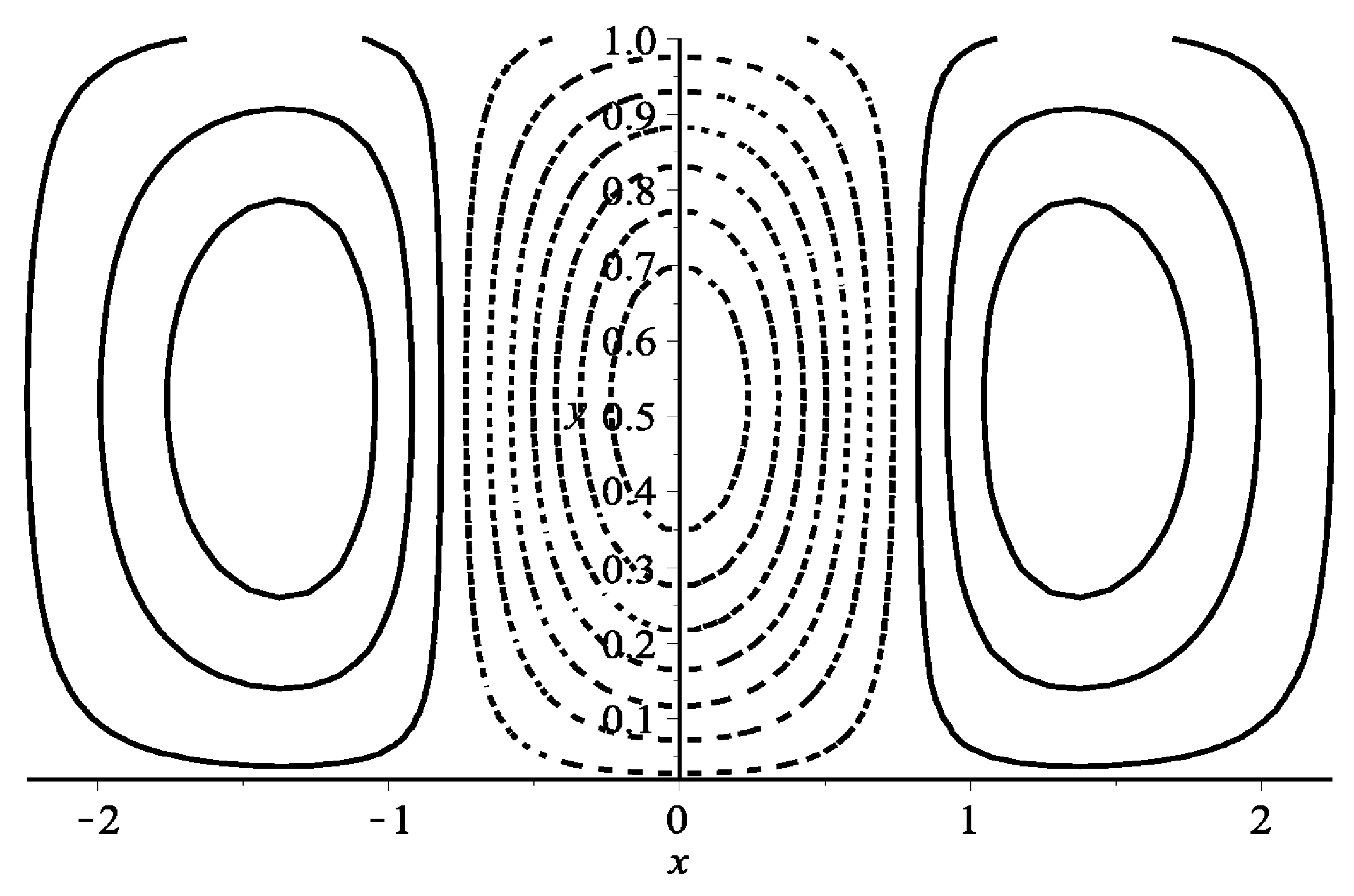
Through an analysis of data, Tao and Ye [26] noted that a warm center is located 15° longitude upstream of a dipole blocking center. The thermal distribution is similar to the perturbation stream field of the unforced form in Equation (8). We could therefore assume that $K{\nabla }^2{\phi }^{\ast }=\mu \psi$, which represent the perturbation terms in Equation (8), where $\mu =C_D{D}_E/H$, $\mu$ and $C_D$ are the coefficients of thermal forcing and sea-level friction, respectively. The thermal distribution shown in Figure 1 is based on this assumption. The center of thermal vorticity is located upstream of the blocking center and the distance between the two thermal vorticities is about 1500 km in the east–west direction, which is consistent with the results of previous data analyses [26,27].

If we let $\Delta T=T_1-T_0$ and $\Delta \tilde{T}=\frac{\Delta T}{\overline{T}}$, then $\Delta \tilde{T}~O({10}^{-2})$. $\mu \sim O({10}^{-2})$, which denotes weak heating in the mid- to high-latitude atmosphere [28]. Thus, we obtained

$$\left\{\begin{array}{l}\epsilon ={({10}^{-1}\mu )}^{\raisebox{1ex}{$1$}\!\left/ \!\raisebox{-1ex}{$2$}\right.},\\ \Delta T^{\prime }=10\Delta \tilde{T}.\end{array}\right.$$

(9)

Then, $\epsilon \ll \Delta T^{\prime }\ll O(1)$ and Equation (8) could be written in the following form:

$$\frac{\partial }{\partial t}{\nabla }^2\psi +\overline{U}\frac{\partial }{\partial x}{\nabla }^2\psi +J(\psi ,{\nabla }^2\psi )+(\beta -\overline{U^{″}})\frac{\partial \psi }{\partial x}={\epsilon }^2\Delta T^{\prime }\psi$$

(10)

Based on the multiscale transformation method [20,24,29], we introduced the following slow coordinates:

$$\tau =\epsilon t, T={\epsilon }^{2}t, X=\epsilon x, \xi ={\epsilon }^{2}x$$

(11)

Considering that $\epsilon$ is a small parameter, $\tau$, $T$, $X$, and $\xi$ are slow variables. According to the results of Ye and Chao [30], $\tau$ represents the large-scale characteristic time, $T$ is the slow exogenous forced characteristic time, $X$ is the longwave characteristic scale, and $\xi$ is the ultra-longwave characteristic scale. A transformation was then performed [24]:

$$\left\{\begin{array}{c}\frac{\partial }{\partial t}\to \frac{\partial }{\partial t}+\epsilon \frac{\partial }{\partial \tau }+{\epsilon }^2\frac{\partial }{\partial T},\\ \frac{\partial }{\partial x}\to \frac{\partial }{\partial x}+\epsilon \frac{\partial }{\partial X}+{\epsilon }^2\frac{\partial }{\partial \xi }.\end{array}\right.$$

(12)

The stream function could then be expanded into a series via the perturbation method [29]:

$$\psi =\epsilon {\psi }_1(x,y,t,X,\xi ,\tau ,T)+{\epsilon }^2{\psi }_2(x,y,t,X,\xi ,\tau ,T)+{\epsilon }^3{\psi }_3(x,y,t,X,\xi ,\tau ,T)+\dots$$

(13)

where ${\psi }_i(i=1,\stackrel{}{}2,\stackrel{}{}3\cdots )$ is the approximation of the $i$th-order perturbation stream function $\psi$.

According to Equation (2), the boundary condition of the perturbation flow could be given as follows:

$$\frac{\partial {\psi }_i}{\partial x}\left|{}_{y=0,\frac{L}{\overline{L}}}\right.=0$$

(14)

Substituting Equations (12) and (13) into Equation (10), all the order problems with respect to $\epsilon$ could be obtained by combining the ${\epsilon }^i(i=1,2,3\cdots )$ like terms.

The $O(\epsilon )$ problem satisfies the equation based on the following linear partial differential equation:

$$O(\epsilon ):K({\psi }_1)\equiv \left(\frac{\partial }{\partial t}+\overline{U}\frac{\partial }{\partial x}\right){\nabla }^2({\psi }_1)+(\beta -{\overline{U}}^{″})\frac{\partial {\psi }_1}{\partial x}=0$$

(15)

where K is a linear operator (similarly hereinafter). The solution of Equation (15) based on the boundary condition of Equation (14) is as follows:

$${\psi }_1=\sqrt{\frac{2}{L}}A(X,\xi ,\tau ,T){\varphi }_1(y)e^{ik(x-ct)}+cc,$$

(16)

where $A$ is a complex amplitude, $k$ and $c$ represent the zonal wavenumber and zonal wave velocity, respectively, and $cc$ signifies the complex conjugate of the preceding term. The eigenvalue problem of ${\varphi }_1$ is governed by an ordinary differential equation with a homogeneous boundary:

$$\left\{\begin{array}{l}\frac{d^2{\varphi }_1}{d{y}^2}{\varphi }_1+\left(\frac{\beta -\overline{U^{″}}}{\overline{U}-c}-k^2\right){\varphi }_1=0,\\ {\varphi }_1(0)={\varphi }_1\left(\frac{L}{\overline{L}}\right)=0.\end{array}\right.$$

The $O({\epsilon }^2)$ problem satisfies the following equation:

$$\begin{array}{ll}O({\epsilon }^2):& K({\psi }_2)=-\left\{\frac{\partial }{\partial \tau }{\nabla }^2{\psi }_1+2\frac{{\partial }^3{\psi }_1}{\partial t\partial x\partial X}+2\overline{U}\frac{{\partial }^3{\psi }_1}{\partial x\partial X}+\overline{U}\frac{\partial }{\partial X}{\nabla }^2{\psi }_1\right.\\ & \left.+\frac{\partial {\psi }_1}{\partial x}\frac{\partial }{\partial y}{\nabla }^2{\psi }_1-\frac{\partial {\psi }_1}{\partial y}\frac{\partial }{\partial x}{\nabla }^2{\psi }_1+(\beta -{\overline{U}}^{″})\right\}.\end{array}$$

(17)

Substituting Equation (16) into Equation (17), we obtained the following nonlinear partial differential equation:

$$\begin{array}{ll}K({\psi }_2)=& -\left\{\left[\frac{\partial A}{\partial \tau }\left(\frac{d^2{\varphi }_1}{d{y}^2}-k^2{\varphi }_1\right)+2k^{2}c{\varphi }_1\frac{\partial A}{\partial X}-2\overline{U}{\varphi }_1\frac{\partial A}{\partial X}+\overline{U}\frac{\partial A}{\partial X}\left(\frac{d^2{\varphi }_1}{d{y}^2}-k^2{\varphi }_1\right)\right.\right.\\ & \left.+(\beta -{\overline{U}}^{″})\frac{\partial A}{\partial X}\right]e^{ik(x-ct)}+\left[ik{\varphi }_1\frac{d}{dy}\right.\left(\frac{d^2{\varphi }_1}{d{y}^2}-k^2{\varphi }_1\right)\\ & \left.\left.-\frac{d{\varphi }_1}{dy}ik\left(\frac{d^2{\varphi }_1}{d{y}^2}-k^2{\varphi }_1\right)\right]A^2{e}^{2ik(x-ct)}+cc\right\}.\end{array}$$

(18)

Because the operator $K$ contains a homogeneous solution of the form $e^{ik(x-ct)}$, the right-hand side of Equation (18) cannot exhibit resonance forcing of the form $e^{ik(x-ct)}$. Therefore, the condition for eliminating the secular term is as follows:

$$\frac{\partial A}{\partial \tau }+c_l\frac{\partial A}{\partial X}=0$$

with $c_l=\frac{\frac{d^2{\varphi }_1}{d{y}^2}-k^2{\varphi }_1}{2k^{2}c{\varphi }_1-2\overline{U}{\varphi }_1+\overline{U}\left(\frac{d^2{\varphi }_1}{d{y}^2}-k^2{\varphi }_1\right)+(\beta -{\overline{U}}^{″})}$.

We could therefore rewrite Equation (17):

$$K({\psi }_2)=ik{A}^{2}G(y)e^{2ik(x-ct)},$$

(19)

where

$$G(y)={\varphi }_1\frac{d}{dy}\left(\frac{d^2{\varphi }_1}{d{y}^2}-k^2{\varphi }_1\right)-\frac{d{\varphi }_1}{dy}\left(\frac{d^2{\varphi }_1}{d{y}^2}-k^2{\varphi }_1\right).$$

According to the boundary conditions of Equations (14) and (19), we could obtain the solution to Equation (19) in the following form:

$${\psi }_2=B(X,\xi ,\tau ,T){\varphi }_2(y)e^{2ik(x-ct)}+cc$$

(20)

By comparing Equations (19) and (20), we obtained the following relationship between $B$ and $A$:

$$B\left((\overline{U}-c)\left(\frac{d^2}{d{y}^2}-k^2\right)+(\beta -{\overline{U}}^{″})\right){\varphi }_2=A^{2}G(y).$$

In this equation, $A$ and $B$ are functions of $X,\xi ,\tau ,T$, and $A$ is proportional to $B$. Then, $B$ could be written in the following form [15,31]:

$$B=A^2$$

(21)

Accordingly, the characteristic equation of ${\varphi }_2$ could be obtained:

$$\left\{\begin{array}{l}\frac{d^2{\varphi }_2}{d{y}^2}+\left(\frac{\beta -\overline{U^{″}}}{\overline{U}-c}-k^2\right){\varphi }_2=\frac{G(y)}{\overline{U}-c},\\ {\varphi }_2(0)={\varphi }_2\left(\frac{L}{\overline{L}}\right)=0.\end{array}\right.$$

The $O({\epsilon }^3)$ problem satisfies the following equation:

$$\begin{array}{ll}O({\epsilon }^3):& K({\psi }_3)=-\{\frac{\partial }{\partial \tau }\left({\nabla }^2{\psi }_2+2\frac{{\partial }^2{\psi }_1}{\partial x\partial X}\right)+\frac{\partial }{\partial t}\left(\frac{{\partial }^2{\psi }_1}{\partial X^2}+2\frac{{\partial }^2{\psi }_2}{\partial x\partial X}+2\frac{{\partial }^2{\psi }_1}{\partial x\partial \xi }\right)\\ & +\frac{\partial }{\partial T}{\nabla }^2{\psi }_1+\left(\frac{\partial {\psi }_2}{\partial x}+\frac{\partial {\psi }_1}{\partial X}\right)\frac{\partial }{\partial y}{\nabla }^2{\psi }_1+\frac{\partial {\psi }_1}{\partial x}\frac{\partial }{\partial y}\left({\nabla }^2{\psi }_2+2\frac{{\partial }^2{\psi }_1}{\partial x\partial X}\right)\\ & -\frac{\partial {\psi }_2}{\partial y}\frac{\partial }{\partial x}{\nabla }^2{\psi }_1-\frac{\partial {\psi }_1}{\partial y}\left[\frac{\partial }{\partial x}\left({\nabla }^2{\psi }_2+2\frac{{\partial }^2{\psi }_1}{\partial x\partial X}\right)+\frac{\partial }{\partial X}{\nabla }^2{\psi }_1\right]\\ & +\overline{U}\left[\frac{{\partial }^3{\psi }_1}{\partial x\partial X^2}+2\frac{{\partial }^3{\psi }_2}{\partial x^2\partial X}+2\frac{{\partial }^3{\psi }_1}{\partial x^2\partial \xi }+\frac{\partial }{\partial X}\left({\nabla }^2{\psi }_2+2\frac{{\partial }^2{\psi }_1}{\partial x\partial X}\right)+\frac{\partial }{\partial \xi }{\nabla }^2{\psi }_1\right]\\ & +(\beta -{\overline{U}}^{″})\left(\frac{\partial {\psi }_2}{\partial X}+\frac{\partial {\psi }_1}{\partial \xi }\right)+\Delta T^{\prime }{\psi }_1\}.\end{array}$$

(22)

For the $O({\epsilon }^3)$ problem (Equation (22)), similar to the $O({\epsilon }^2)$ problem, the condition of eliminating the secular term about $O({\epsilon }^3)$ could be obtained by removing the resonance term. The equation about the amplitude $A$ could be obtained from Equation (21) because the condition for eliminating the secular term contains the formula about $B$:

$$\frac{\partial A}{\partial t}+c_g\frac{\partial A}{\partial x}-i\lambda \frac{{\partial }^{2}A}{\partial x^2}-i{\epsilon }^2\delta {\left|A\right|}^{2}A-\gamma \Delta T^{\prime }A=0,$$

(23)

where $i^2=-1$, $c_g=\frac{I_1}{I},\lambda =\frac{I_2}{I},\delta =\frac{I_3}{I},\gamma =\frac{I_4}{I}$, and

$$I={\displaystyle {\int }_0^{\raisebox{1ex}{$L$}\!\left/ \!\raisebox{-1ex}{$\overline{L}$}\right.}{\varphi }_1{}^2}dy,I_1={\displaystyle {\int }_0^{\raisebox{1ex}{$L$}\!\left/ \!\raisebox{-1ex}{$\overline{L}$}\right.}{c}_l{\varphi }_1{}^2}dy,I_2=k{\displaystyle {\int }_0^{\raisebox{1ex}{$L$}\!\left/ \!\raisebox{-1ex}{$\overline{L}$}\right.}\frac{\overline{U}-c}{\beta -{\overline{U}}^{″}}[3\overline{U}-(c+2c_l)]{\varphi }_1{}^2}dy,$$

$$I_3=k{\displaystyle {\int }_0^{\raisebox{1ex}{$L$}\!\left/ \!\raisebox{-1ex}{$\overline{L}$}\right.}\frac{\overline{U}-c}{\beta -{\overline{U}}^{″}}\left\{-{\varphi }_1{}^2{\varphi }_2\left(\frac{\beta -{\overline{U}}^{″}}{\overline{U}-c}\right)-\frac{{\varphi }_1{}^2}{2}\frac{d}{dy}\left(\frac{G}{\overline{U}-c}\right)-\frac{G{\varphi }_1}{\overline{U}-c}\frac{d{\varphi }_1}{dy}\right\}}dy,$$

$$I_4={\displaystyle {\int }_0^{\raisebox{1ex}{$L$}\!\left/ \!\raisebox{-1ex}{$\overline{L}$}\right.}\frac{(\overline{U}-c){\varphi }_1}{\beta -{\overline{U}}^{″}}\left(\frac{d^2{\varphi }_2}{d{y}^2}-k^2{\varphi }_2\right)}dy.$$

In the following section, we discuss the geometric structure of the flow field of the dipole blocking and the influence of the anomalous thermal vorticity in the Arctic on its structure based on the amplitude of the perturbation (Equation (23)) in the quasi-geostrophic flow.

3. Dipole Blocking Structure without Thermal Forcing

Before discussing the effect of Arctic warming on the dipole blocking structure, we need to understand the topological structure of dipole blocking without thermal forcing. The following equation can be obtained after establishing $\varsigma =\sqrt{\delta /2\lambda }(x-c_{g}t)$, $t^{\prime }=\frac{\delta }{2}t$, and $M=\epsilon A$:

$$i\frac{\partial M}{\partial t^{\prime }}+\frac{{\partial }^{2}M}{\partial {\varsigma }^2}+2{\left|M\right|}^{2}M-i\gamma \Delta T^{\prime }M=0$$

(24)

Considering $t^{\prime }$ as $t$, Equation (24) becomes

$$i\frac{\partial M}{\partial t}+\frac{{\partial }^{2}M}{\partial {\varsigma }^2}+2{\left|M\right|}^{2}M-i\gamma \Delta T^{\prime }M=0$$

(25)

Without thermal forcing (i.e., $\gamma =0$), Equation (25) is a standard nonlinear Schrӧdinger equation, for which there is the following single-soliton case:

$$M_0(\varsigma ,t)=2{\alpha }_0\sec \mathrm{h}[2{\chi }_0(\varsigma -{\varsigma }_0+4{\chi }_{0}t)]\exp [-2i{\chi }_0\varsigma -4i({\chi }_0^2-{\alpha }_0^2)t-i{\theta }_0]$$

(26)

where ${\alpha }_0$, ${\chi }_0$, ${\varsigma }_0$, and ${\theta }_0$ are real parameters. ${\alpha }_0$ and ${\chi }_0$ represent the amplitude and velocity of the soliton, respectively, whereas ${\varsigma }_0$ and ${\theta }_0$ represent the initial position and initial phase of the soliton, respectively. If $\overline{U}(y)={\overline{U}}_0$, then the corresponding stream function becomes

$$\begin{array}{c}\psi =-{\overline{U}}_{0}y+2\epsilon {\alpha }_0\sec \mathrm{h}\left\{2{\alpha }_0\left(\sqrt{\frac{\delta }{2\lambda }}(x-x_0-\frac{\delta c_g}{2}t)+4{\chi }_{0}t\right)\right\}\sin my\\ \times \exp \left\{-2i{\chi }_0\sqrt{\frac{\delta }{2\lambda }}(x-\frac{\delta c_g}{2}t)-2\delta i({\chi }_0^2-{\alpha }_0^2)t-i{\theta }_0\right\}+cc.\end{array}$$

(27)

Because the initial phase ${\theta }_0$ can only change the position of the soliton center, the amplitude and structure of the soliton cannot be changed. The initial position $x_0$ can only alter the center position and amplitude of the soliton, not its structure. The flow structure for $x_0=0$ and ${\theta }_0=0$ is discussed without loss of generality. Given that $cc$ is in a conjugate form, Equation (27) can be written as:

$$\psi =-{\overline{U}}_{0}y+4\epsilon {\alpha }_0\sec \mathrm{h}\left(2{\alpha }_0{}^{\prime }\right)\sin my\cos \left(2{\chi }_0{}^{\prime }\right)$$

(28)

where ${\alpha }_0{}^{\prime }={\alpha }_0\left(\sqrt{\delta /2\lambda }(x-\delta c_{g}t/2)\right)+2{\chi }_{0}t$ and ${\chi }_0{}^{\prime }={\chi }_0\sqrt{\delta /2\lambda }(x-\delta c_{g}t/2t)-\delta ({\chi }_0^2-{\alpha }_0^2)t$. Given the relations of the stream function $\psi$ with the zonal velocity $u$ and meridional velocity $v$, the following vector equation can be obtained:

$$\left\{\begin{array}{l}\frac{dx}{dt}=u=-\frac{\partial \psi }{\partial y}=4\epsilon {\alpha }_{0}m\sec \mathrm{h}\left({\alpha }_0{}^{\prime }\right)\cos \left({\chi }_0{}^{\prime }\right)\sin my+{\overline{U}}_0,\\ \frac{dy}{dt}=v=\frac{\partial \psi }{\partial x}=-4\epsilon {\alpha }_0\left({\alpha }_0{}^{\prime }\tan \mathrm{h}\left({\alpha }_0{}^{\prime }\right)\cos \left({\chi }_0{}^{\prime }\right)+{\chi }_0\sin \left({\chi }_0{}^{\prime }\right)\right)\cos my.\end{array}\right.$$

(29)

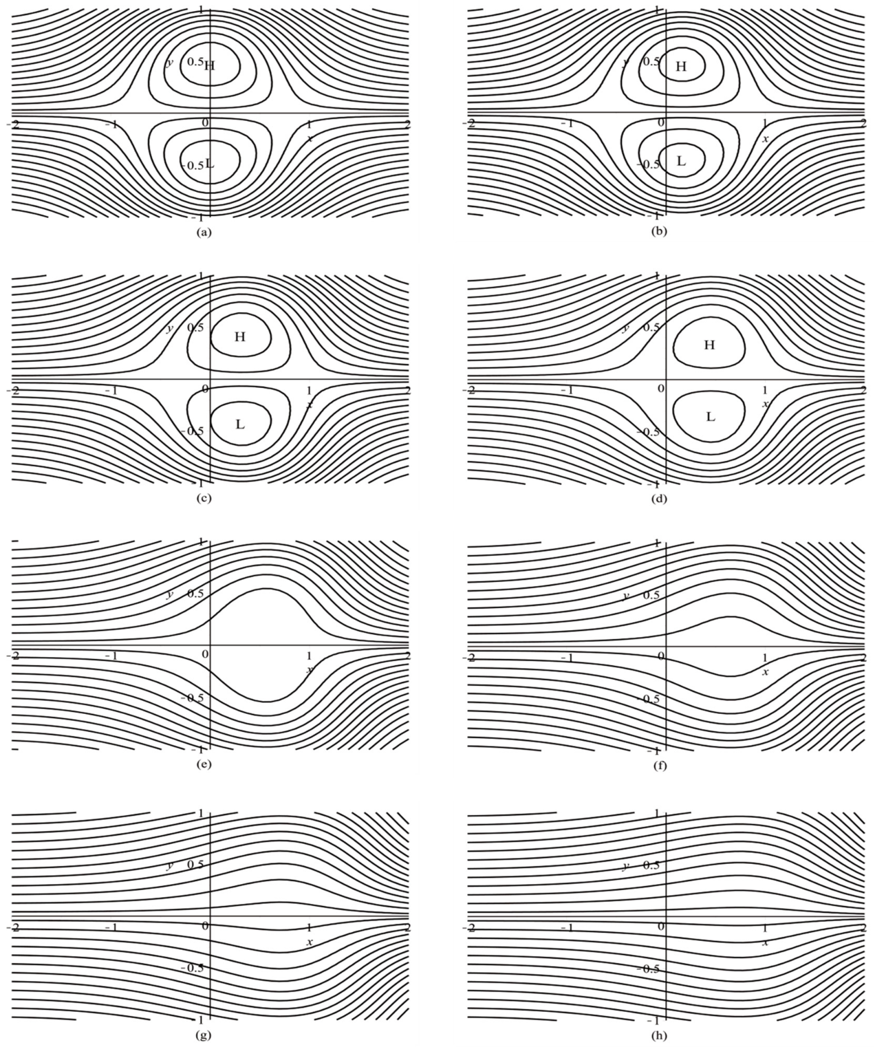
According to the characteristics of the average zonal wind velocity in Equations (29), (7), (9), and (11), ${\alpha }_0=\sqrt{{\nu }_0/2\delta }\approx 1500$ km was determined after establishing $L=3000$ km, $\overline{L}=6000$ km, $\overline{V}=10$ m/s, ${\overline{U}}_0=8$ m/s, and $m=2$ [15]. The corresponding flow then followed the dipole blocking flow (Figure 2).

Because the wave amplitude of the dipole blocking flow increases monotonically with ${\alpha }_0{}^{\prime }$ and $\left({\alpha }_0\delta c_g\sqrt{\delta /2\lambda }\right)/2>2{\chi }_0$, the dipole blocking flow is dispersive. From this analysis, the effect of the zonal wind velocity on the dipole blocking structure can explain why the development of planetary waves tends to be accompanied by low wind velocities when a meridional circulation prevails. Equation (29) shows that with a certain number of waves ($m$) and an average zonal velocity (${\overline{U}}_0$), the amplitude $\alpha$ of the soliton determines the type of flow field and is not related to the velocity $\chi$ of the soliton. From this analysis, a blocked flow field is formed under the nonlinear action of the atmosphere without thermal forcing. Under the effect of dipole blocking on the flow field, the movement of Arctic cold air toward the south is conducive to the formation of cold air or cold waves over Eurasia in winter. The Arctic has experienced significant warming in recent years and a warm Arctic–cold Eurasian temperature distribution often appears. To explain this phenomenon, we need to theoretically prove that Arctic warming in winter strengthens dipole blocking and contributes to the abnormal distribution of warm Arctic–cold Eurasian temperatures. Therefore, the effect of decreasing the absolute value of the difference in temperature ($\Delta T=T_1-T_0$) between the Arctic and midlatitudes on dipole blocking was studied through the influence of the thermal forcing terms on the Schrӧdinger soliton.

4. Impact of Thermal Forcing on the Schrӧdinger Equation for Solitons

Because $\Delta T^{\prime }\sim O({10}^{-1})$ and $\gamma \sim O(1)$, the thermal forcing term in Equation (24) is of the $O({10}^{-1})$ order of magnitude, namely, $\gamma \Delta T^{\prime }\sim O({10}^{-1})$, which can be considered as a small term. Therefore, we discuss the effect of thermal forcing on dipole blocking by analyzing the effect of a perturbation on the amplitude of the soliton. To use the direct approach to perturbation theory for solitons to analyze the effect of atmospheric thermal forcing on the nonlinear Schrӧdinger equation, we rewrote Equation (25) in the following form:

$$i\frac{\partial M}{\partial t}+\frac{{\partial }^{2}M}{\partial {\varsigma }^2}+2{\left|M\right|}^{2}M=i{\gamma }^{\prime }f[M],$$

(30)

with ${\gamma }^{\prime }=0.1\gamma$, $f[M]=\Delta T^{″}M$, $\Delta T^{″}=10\Delta T^{\prime }$, and $\Delta T^{″}\sim O(1)$.

For Equation (30), we sought a first-order approximate solution, as follows:

$$M(\varsigma ,t)=M_0(\varsigma ,t)+{\gamma }^{\prime }S(\varsigma ,t),$$

(31)

with the initial conditions $M(\varsigma ,0)=M_0(\varsigma ,0),S(\varsigma ,0)=0$, where $M_0(\varsigma ,t)$ represents the zero-order term and $S(\varsigma ,t)$ represents the first-order term. Furthermore, to eliminate the so-called secular terms, we introduced a slow time variable:

$$\mathsf{\Pi }={\gamma }^{\prime }t$$

(32)

The derivative with respect to $t$ then became

$$\frac{\partial }{\partial t}\to \frac{\partial }{\partial t}+{\gamma }^{\prime }\frac{\partial }{\partial \mathsf{\Pi }}$$

(33)

By substituting Equations (31)–(33) into Equation (30), the first-order term $S(\varsigma ,t)$ was linearized into the following equations (with appropriate initial conditions):

$$\left\{\begin{array}{l}i\frac{\partial M_0}{\partial t}+\frac{{\partial }^2{M}_0}{\partial {\varsigma }^2}+2{\left|M_0\right|}^2{M}_0=0,\\ M_0(\varsigma ,0)=2{\alpha }_0\sec \mathrm{h}[2{\chi }_0(\varsigma -{\varsigma }_0)]\exp (-2i{\chi }_0\varsigma -i{\theta }_0),\end{array}\right.$$

(34)

and

$$\left\{\begin{array}{l}i\frac{\partial S}{\partial t}+\frac{{\partial }^{2}S}{\partial {\varsigma }^2}+4{\left|M_0\right|}^{2}S+2M_0^2\overline{S}=if[M_0]-i\frac{\partial M_0}{\partial \mathsf{\Pi }}\equiv ir[M_0],\\ S(\varsigma ,0)=0,\end{array}\right.$$

(35)

where an overbar signifies a complex conjugate. The zero-order approximation in Equation (34) is simply the standard nonlinear Schrӧdinger equation, which has a single-soliton solution that is formally the same as that for Equation (26):

$$M_0(\varsigma ,t)=2\alpha e^{-i\theta }\sec \mathrm{h}(z),$$

(36)

with

$$\left\{\begin{array}{l}z=2\alpha (\varsigma -\zeta ),\\ \theta =2\chi (\varsigma -\zeta )+\delta =\chi z/\alpha +\delta ,\\ {\zeta }_t=-4\chi ,\\ {\iota }_t=-4({\alpha }^2+{\chi }^2).\end{array}\right.$$

The soliton parameters $\alpha ,\chi ,\zeta$, and $\iota$ were hypothesized to be functions of the slow time variable $\mathsf{\Pi }$, but $\alpha$ and $\chi$ are independent of $t$. It then follows from Equation (36) that

$$\frac{\partial M_0}{\partial \mathsf{\Pi }}=e^{-i\theta }(2i\alpha (2\chi {\zeta }_t-{\delta }_{\mathsf{\Pi }}){\varphi }^{(1)}(z)-2i{\chi }_{\mathsf{\Pi }}{\varphi }^{(2)}(z)+2{\alpha }_{\mathsf{\Pi }}{\varphi }^{(3)}(z)+4{\alpha }^2{\zeta }_{\mathsf{\Pi }}{\varphi }^{(4)}(z))$$

(37)

where

$$\left\{\begin{array}{l}{\varphi }^{(1)}(z)=\sec \mathrm{h}(z),\\ {\varphi }^{(2)}(z)=z\sec \mathrm{h}(z),\\ {\varphi }^{(3)}(z)=(1-z\tan \mathrm{h}(z))\sec \mathrm{h}(z),\\ {\varphi }^{(4)}(z)=\tan \mathrm{h}(z)\sec \mathrm{h}(z).\end{array}\right.$$

It was convenient to use the independent variable $z$. Therefore, substituting Equation (33) into Equation (35) and its complex conjugate equation led to the following:

$$\left\{\begin{array}{l}i\frac{\partial S}{\partial t}+8i\alpha \chi \frac{\partial S}{\partial z}+4{\alpha }^2\frac{{\partial }^{2}S}{\partial z^2}+16{\alpha }^2{\sec \mathrm{h}}^2(z)S+8{\alpha }^2{\sec \mathrm{h}}^2(z)e^{-2i\theta }\overline{S}=ir,\hspace{1em}S(z,0)=0,\\ i\frac{\partial \overline{S}}{\partial t}+8i\alpha \chi \frac{\partial \overline{S}}{\partial z}-4{\alpha }^2\frac{{\partial }^2\overline{S}}{\partial z^2}-16{\alpha }^2{\sec \mathrm{h}}^2(z)\overline{S}-8{\alpha }^2{\sec \mathrm{h}}^2(z)e^{2i\theta }S=i\overline{r},\hspace{1em}\overline{S}(z,0)=0.\end{array}\right.$$

(38)

The following forms were allowed:

$$S=e^{-i\theta }w,\overline{S}=e^{i\theta }\overline{w}$$

Equation (38) could then be written as a matrix:

$$i\frac{\partial W}{\partial t}+4{\alpha }^{2}LW=i{e}^{i{\sigma }_3\theta }R,W(z,0)=0,$$

(39)

where ${\sigma }_3=\left[\begin{array}{cc}1& 0\\ 0& -1\end{array}\right]$, which is called the third Pauli matrix; $W$ and $R$ are two-dimensional column matrices; and $L$ represents a $2\times 2$ matrix. They are defined as follows:

$$W=\left[\begin{array}{c}w\\ \overline{w}\end{array}\right], R=\left[\begin{array}{c}r\\ \overline{r}\end{array}\right],$$

$$L=\left[\begin{array}{cc}\frac{{\partial }^2}{\partial z^2}+4{\sec \mathrm{h}}^2(z)-1& 2{\sec \mathrm{h}}^2(z)\\ -2{\sec \mathrm{h}}^2(z)& -\frac{{\partial }^2}{\partial z^2}-4{\sec \mathrm{h}}^2(z)+1\end{array}\right]$$

Because Equation (39) is a separable partial differential equation with a zero boundary, it can be solved by the Sturm–Liouville eigenvalue theory. According to the Sturm–Liouville eigenvalue theory of linear operator equations, the sequences of the real eigenvalues and eigenfunctions of the linear operator $L$ and its adjoint operator $L^{*}$ can be obtained. $W$ can then be constituted by the complete orthogonal basis functions spanned by these eigenfunctions.

To obtain the solution of the variable ($W$) in Equation (39), the key was to solve the following two eigenvalue problems:

$$L\mathsf{\Phi }=\rho \mathsf{\Phi }, L^{*}\mathsf{\Psi }={\rho }^{*}\mathsf{\Psi },$$

(40)

where $L^{*}$ is the adjoint operator of $L$, $\rho$ and ${\rho }^{*}$ are the eigenvalues of $L$ and $L^{*}$, respectively, $\mathsf{\Phi }$ is the eigenfunction of $\widehat{L}$ with respect to $\rho$, and $\mathsf{\Psi }$ is the eigenfunction of $L^{*}$, which is defined as

$$L^{\ast }=\left[\begin{array}{cc}\frac{{\partial }^2}{\partial z^2}+4{\sec \mathrm{h}}^2(z)-1& -2{\sec \mathrm{h}}^2(z)\\ 2{\sec \mathrm{h}}^2(z)& -\frac{{\partial }^2}{\partial z^2}-4{\sec \mathrm{h}}^2(z)+1\end{array}\right].$$

In addition, the operator $L$ and its adjoint operator $L^{*}$ have the same continuous spectrum [32]. Given $\sec {\mathrm{h}}^2(z)\to 0 \mathrm{when} z\to \pm \infty$, then

$$L\to \left[\begin{array}{cc}\frac{{\partial }^2}{\partial z^2}-1& 0\\ 0& -\frac{{\partial }^2}{\partial z^2}+1\end{array}\right], \mathrm{when} \mathrm{z}\to \pm \infty .$$

Therefore, the eigenvalues of operator $L$ and its adjoint operator $L^{*}$ can be obtained:

$$\rho ={\rho }^{*}=\pm \stackrel{}{}(k^2+1),\hspace{1em}-\infty <k<\infty ,$$

where $k$ is a real number. Correspondingly, the orthogonal basis of Equation (40) is as follows:

$$\begin{array}{l}\left\{\mathsf{\Phi }\right\}=\{{\mathsf{\Phi }}^{+}(z,k), {\mathsf{\Phi }}^{-}(z,k), {\mathsf{\Phi }}^j(z); j=1, 2, 3, 4\},\\ \left\{\mathsf{\Psi }\right\}=\{{\mathsf{\Psi }}^{+}(z,k), {\mathsf{\Psi }}^{-}(z,k), {\mathsf{\Psi }}^j(z); j=1, 2, 3, 4\},\end{array}$$

with

$$\begin{array}{l}{\mathsf{\Phi }}^{+}(z,k)=\frac{e^{ikz}}{\sqrt{2\pi }(k^2+1)}\left[\begin{array}{c}-{\sec \mathrm{h}}^2(z)\\ {(\tan z-ik)}^2\end{array}\right],{\mathsf{\Phi }}^{-}(z,k)=\frac{e^{ikz}}{\sqrt{2\pi }(k^2+1)}\left[\begin{array}{c}{(\tan z-ik)}^2\\ -{\sec \mathrm{h}}^2(z)\end{array}\right],\\ {\mathsf{\Psi }}^{+}(z,k)=\frac{e^{ikz}}{\sqrt{2\pi }(k^2+1)}\left[\begin{array}{c}{\sec \mathrm{h}}^2(z)\\ {(\tan z-ik)}^2\end{array}\right],{\mathsf{\Psi }}^{-}(z,k)=\frac{e^{ikz}}{\sqrt{2\pi }(k^2+1)}\left[\begin{array}{c}{(\tan z-ik)}^2\\ {\sec \mathrm{h}}^2(z)\end{array}\right],\end{array}$$

$$\begin{array}{l}{\mathsf{\Phi }}^1(z)=\frac{1}{\sqrt{2}}{\varphi }^{(1)}(z)\left[\begin{array}{c}1\\ -1\end{array}\right],{\mathsf{\Phi }}^2(z)=\frac{1}{\sqrt{2}}{\varphi }^{(2)}(z)\left[\begin{array}{c}1\\ -1\end{array}\right],\\ {\mathsf{\Phi }}^3(z)=\frac{1}{\sqrt{2}}{\varphi }^{(3)}(z)\left[\begin{array}{c}1\\ 1\end{array}\right],{\mathsf{\Phi }}^4(z)=\frac{1}{\sqrt{2}}{\varphi }^{(4)}(z)\left[\begin{array}{c}1\\ 1\end{array}\right],\end{array}$$

$$\begin{array}{l}{\mathsf{\Psi }}^1(z)=\frac{1}{\sqrt{2}}{\varphi }^{(3)}(z)\left[\begin{array}{c}1\\ -1\end{array}\right],{\mathsf{\Psi }}^2(z)=\frac{1}{\sqrt{2}}{\varphi }^{(4)}(z)\left[\begin{array}{c}1\\ -1\end{array}\right],\\ {\mathsf{\Psi }}^3(z)=\frac{1}{\sqrt{2}}{\varphi }^{(1)}(z)\left[\begin{array}{c}1\\ 1\end{array}\right],{\mathsf{\Psi }}^4(z)=\frac{1}{\sqrt{2}}{\varphi }^{(2)}(z)\left[\begin{array}{c}1\\ 1\end{array}\right].\end{array}$$

Expanding $W$ with the basis function $\left\{\mathsf{\Phi }\right\}$, we obtained the following equation:

$$W(z,t)={\displaystyle {\int }_{-\infty }^{\infty }\{a^{+}(t,k){\mathsf{\Phi }}^{+}+a^{-}(t,k){\mathsf{\Phi }}^{-}\}dk}+{\displaystyle \sum _{j=1}^4{a}^j(t){\mathsf{\Phi }}^j},$$

(41)

where $a^{+}(t,k)$, $a^{-}(t,k)$, and $a^j(t)\stackrel{}{}(j=1,\stackrel{}{}2,\stackrel{}{}3,\stackrel{}{}4)$ represent expansion coefficients.

By substituting Equation (41) into Equation (39), the coefficient of which is a function of only $t$ after integration, Equation (39) could be separated into ordinary differential equations about the expansion coefficients $a^{+}(t,k)$, $a^{-}(t,k)$, and $a^j(t)\stackrel{}{}(j=1,\stackrel{}{}2,\stackrel{}{}3,\stackrel{}{}4)$ [33,34].

$$\{\begin{array}{l}i\frac{d{a}^{\pm }(t,k)}{dt}\pm 4{\beta }^2(k^2+1)a^{\pm }(t,k)=i{\displaystyle {\int }_{-\infty }^{\infty }dz}\overline{{\mathsf{\Psi }}^{\pm }(z,k)}{e}^{i{\sigma }_3\theta }R[M_0(z)],\hspace{1em}{a}^{\pm }(0,k)=0,\\ i\frac{d{a}^1(t,k)}{dt}+8{\beta }^2{a}^3(t)=i{\displaystyle {\int }_{-\infty }^{\infty }dz}\overline{{\mathsf{\Psi }}^1(z)}{e}^{i{\sigma }_3\theta }R[M_0(z)],\hspace{1em}{a}^1(0)=0,\\ i\frac{d{a}^2(t,k)}{dt}=i{\displaystyle {\int }_{-\infty }^{\infty }dz}\overline{{\mathsf{\Psi }}^2(z)}{e}^{i{\sigma }_3\theta }R[M_0(z)],\hspace{1em}{a}^2(0)=0,\\ i\frac{d{a}^3(t,k)}{dt}=i{\displaystyle {\int }_{-\infty }^{\infty }dz}\overline{{\mathsf{\Psi }}^3(z)}{e}^{i{\sigma }_3\theta }R[M_0(z)],\hspace{1em}{a}^3(0)=0,\\ i\frac{d{a}^4(t,k)}{dt}-8{\beta }^2{a}^2(t)=i{\displaystyle {\int }_{-\infty }^{\infty }dz}\overline{{\mathsf{\Psi }}^4(z)}{e}^{i{\sigma }_3\theta }R[M_0(z)],\hspace{1em}{a}^4(0)=0.\end{array}$$

(42)

According to Equations (42) and (37), the terms $a^{+}(t,k)$, $a^{-}(t,k)$, and $a^j(t)\stackrel{}{}(j=1,\stackrel{}{}2,\stackrel{}{}3,\stackrel{}{}4)$ can be solved. The expression of $W$ and $S$ is then known. Substituting $S$ into Equation (38) and differentiating Equation (38) to $\mathsf{\Pi }$, the formulas for the variations in the soliton amplitude ($\alpha$) and velocity ($\chi$) with a slow time variable ($\mathsf{\Pi }$) can be obtained:

$$\left\{\begin{array}{l}\frac{d\alpha }{d\mathsf{\Pi }}=-\frac{1}{2\sqrt{2}}{\displaystyle {\int }_{-\infty }^{\infty }\{{\overline{{\mathsf{\Psi }}^3(z)}}^T{e}^{i{\sigma }_3\theta }F[M_0(z)]\}dz,}\\ \frac{d\chi }{d\mathsf{\Pi }}=\frac{1}{2\sqrt{2}i}{\displaystyle {\int }_{-\infty }^{\infty }\{{\overline{{\mathsf{\Psi }}^2(z)}}^T{e}^{i{\sigma }_3\theta }F[M_0(z)]\}dz,}\end{array}\right.$$

(43)

with

$$F[M_0(z)]=\left[\begin{array}{c}f[M_0]\\ \overline{f[M_0]}\end{array}\right].$$

After obtaining Equation (43) for the effects of perturbations on solitons, we can now discuss the effect of Arctic warming on dipole blocking using Equation (43).

5. Impact of Arctic Warming on Dipole Blocking

To further discuss the impact of Arctic warming on dipole blocking, we substituted the thermal forcing term $f[M]=\Delta T^{″}M$ into Equation (43) and used the following formula computed by the residue theorem [35]:

$$\begin{array}{l}{I}_1(k)={\displaystyle {\int }_{-\infty }^{\infty }{e}^{ikz}\sec \mathrm{h}(z})dz=\frac{\pi }{\cos \mathrm{h}\left(\pi k/2\right)}\\ I_2(k)={\displaystyle {\int }_{-\infty }^{\infty }{e}^{ikz}\tan \mathrm{h}(z)\sec hz}dz=\frac{ik\pi }{\cos \mathrm{h}\left(\pi k/2\right)}\end{array}$$

We then further considered the following matrix-order power formula:

$$e^{{\sigma }_3}=E+{\sigma }_3+\frac{{\sigma }_3^2}{2!}+\cdots +\frac{{\sigma }_3^n}{n!}+\cdots .$$

We could obtain the relation between the motion velocity of the soliton and the slow time variable $\mathsf{\Pi }$ by solving Equation (43):

$$\frac{d\chi }{d\mathsf{\Pi }}=0$$

(44)

Equation (44) signifies that $\chi$ is steady with respect to the slow time variable $\mathsf{\Pi }$. Therefore, we could obtain the variation in the amplitude $\alpha$ of the soliton with regard to the slow time variable $\mathsf{\Pi }$:

$$\frac{d\alpha }{d\mathsf{\Pi }}=2\Delta T^{″}\alpha$$

(45)

According to Equation (45), $\alpha$ increases monotonically about $\Delta T^{″}$.

In general, the temperature difference between the Arctic and midlatitudes at 500 hPa is less than zero ($\Delta T<0$). Equation (45) can then be rewritten as:

$$\frac{d\alpha }{d\mathsf{\Pi }}=-200\frac{\left|\Delta T\right|}{\overline{T}}\alpha$$

(46)

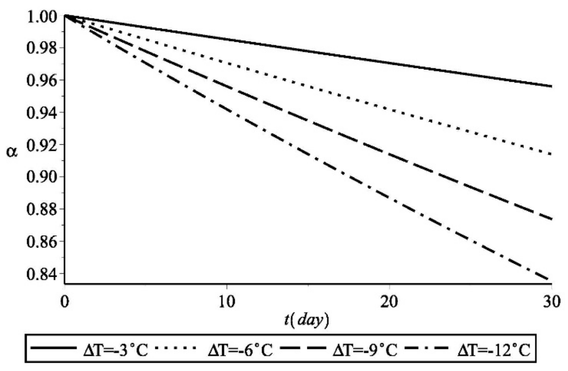
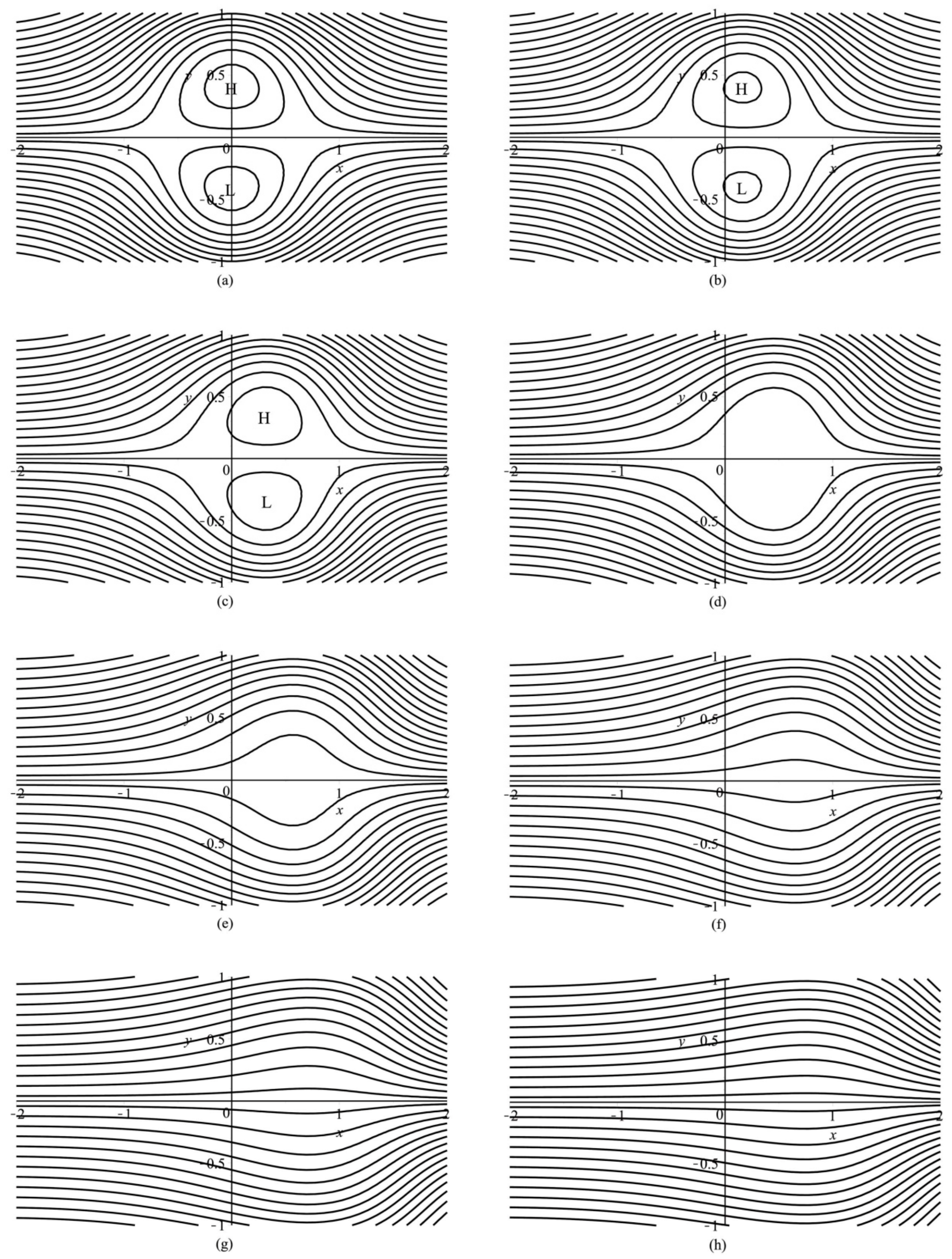
According to Equation (46), the soliton amplitude decays slowly with time under the action of thermal forcing. In other words, the temperature distribution of midlatitude warming and Arctic cooling has an inhibitory effect on the development of blocking during the maintenance phase of dipole blocking. Further analysis shows that the decay rate of the amplitude of the soliton is positively proportional to $\left|\Delta T\right|$—that is, the greater the temperature difference $\left|\Delta T\right|$, the faster the amplitude of the soliton will decrease. Based on this analysis, a decrease in the absolute difference in temperature between the Arctic and Eurasia—namely, $\left|\Delta T\right|$—is conducive to the development of a blocking dipole.

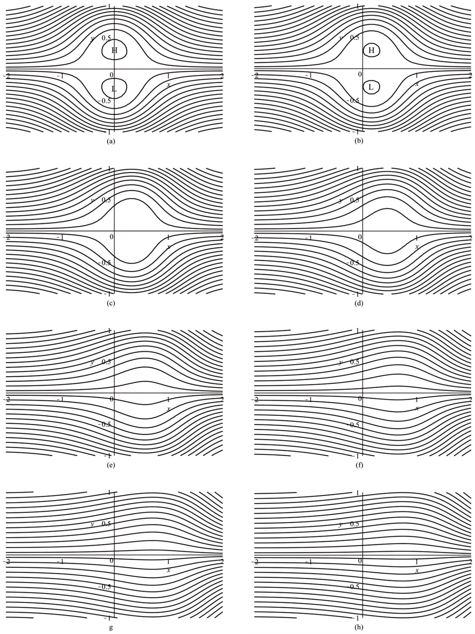
Similar to the analysis in Section 3, $L=3000$ km, $\overline{L}=6000$ km, $\overline{V}=10$ m/s, ${\overline{U}}_0=8$ m/s, and $m=2$ were established [15]. Then, $\gamma =1.4$, ${\alpha }_0=\sqrt{{\nu }_0/2\delta }\approx 1500\mathrm{km}$, $\iota =-1$ and ${\chi }_0=0.31\mathrm{m}/\mathrm{s}$, $\overline{T}=-23.8745$ °C, and Equations (7), (9), (11), and (32) were used to obtain the growth trend for the amplitude of the soliton (Figure 3) when the temperature difference $\Delta T$ is −3, −6, −9, and −12 °C and to obtain the dipole blocking flow when $\Delta T=-12$ °C (Figure 4) and $\Delta T=-9$ °C (Figure 5).

This analysis shows that if there is a perturbation in the zonal flow, the nonlinear interactions between waves and flows within the westerly zone in the northern hemisphere probably induce dipole blocking of the Schrödinger solitons. In addition, the distribution of lower Arctic and higher midlatitude temperatures inhibits the development of solitons. The decrease in the absolute difference in temperature between the Arctic and Eurasia originating from Arctic warming weakens the inhibitory effect on dipole blocking—that is, dipole blocking becomes stronger and lasts for longer as the Arctic warms. It is easy to stimulate the generation of dipole blocking structures over the Ural Mountains, Lake Baikal, and the Okhotsk Sea [15] due to the shear in the zonal base flow caused by the large-scale compulsive action of the Tibetan Plateau, which further strengthens dipole blocking over Eurasia as the Arctic warms.

In January 2008, for example, the Arctic temperature at a 2-m height over a wide area showed positive anomalies, particularly over the Barents–Kara Sea. This caused the westerlies in mid- to high latitudes to weaken [36,37] and formed an anomalous dipole consisting of a Ural blocking high and a low-pressure center over Eurasia, causing the northern branch of the circulation in the Urals to develop strongly toward the Arctic. The northern branch of the circulation then turned south from the Arctic, guiding the cold air of the Arctic in a southeasterly direction to invade East Asia (Figure 6), causing the extremely cold event recorded over eastern China in January 2008.

6. Discussion and Conclusions

We simplified the barotropic modes of thermal forcing for the difference in temperature between the Arctic and midlatitude regions as a nonlinear Schrӧdinger equation with perturbation terms using the multiscale perturbation method. By using the direct approach to perturbation theory for solitons, the effect of Arctic warming in winter was shown to reinforce the blocking dipole in Eurasia, leading to anomalies in winter temperatures in the midlatitudes of Eurasia. The results can be summarized by the following points.

(1)

If only nonlinear effects between waves and zonal flows exist, then the atmospheric circulation in the westerly air flow can present a blocking structure.

(2)

The temperature gradient formed by warming in midlatitude regions and cooling in the Arctic inhibits the development of blocking dipole structures.

(3)

The inhibitory effect on the development of a blocking dipole is weakened by Arctic warming, which has led to smaller temperature gradients between the Arctic and midlatitude regions in the last few decades. As a consequence, blocking dipole structures are generated with relative ease and the cold air over the Arctic is more easily transported southward, resulting in anomalously low winter temperatures in midlatitudes, especially in regions with initial blocking dipole conditions (such as the Ural Mountains and Lake Baikal).

These conditions can trigger regionally cold events at mid- and even lower latitudes over some regions of Eurasia. This study has therefore confirmed theoretically the results of previous observations and data analyses (e.g., [1,2,3,4,7]), although two problems still need to be resolved. First, the association between Arctic warming and a blocking dipole is based on an idealized barotropic model solution, which requires more supporting experimental data and the addition of a baroclinic component for further study. Second, as a result of the evolution of the blocking dipole, the barotropic or baroclinic structure of the atmospheric circulation tends to change. Under normal circumstances, the baroclinic structure in the development stage will evolve into a blocking dipole with an equivalent barotropic structure in the maintenance stage and is then converted into a baroclinic structure during the decay stage. The equivalent barotropic structure in the maintenance stage can be considered as an approximation of the baroclinic structure (where the shear between the upper and lower approach is zero). Therefore, it is necessary to study the formation, maintenance, decrease, and re-formation of the blocking dipole under the framework of a baroclinic atmosphere. The thermodynamic and dynamic processes determining the effects of Arctic warming on the weather and climate can then be explored in mid- to high-latitude regions.