Understanding and Predicting Nonlinear Turbulent Dynamical Systems with Information Theory

Abstract

Complex nonlinear turbulent dynamical systems are ubiquitous in many areas. Quantifying the model error and model uncertainty plays an important role in understanding and predicting complex dynamical systems. In the first part of this article, a simple information criterion is developed to assess the model error in imperfect models. This effective information criterion takes into account the information in both the equilibrium statistics and the temporal autocorrelation function, where the latter is written in the form of the spectrum density that permits the quantification via information theory. This information criterion facilitates the study of model reduction, stochastic parameterizations, and intermittent events. In the second part of this article, a new efficient method is developed to improve the computation of the linear response via the Fluctuation Dissipation Theorem (FDT). This new approach makes use of a Gaussian Mixture (GM) to describe the unperturbed probability density function in high dimensions and avoids utilizing Gaussian approximations in computing the statistical response, as is widely used in the quasi-Gaussian (qG) FDT. Testing examples show that this GM FDT outperforms qG FDT in various strong non-Gaussian regimes.

1. Introduction

Complex nonlinear turbulent dynamical systems are ubiquitous in geophysics, engineering, neuroscience, and material science [1,2,3,4,5,6,7,8]. Key features of these complex nonlinear systems include, but are not limited to, multiscale dynamics, high dimensional phase space, nonlinear energy transfers, highly non-Gaussian Probability Density Functions (PDFs), intermittent instability, random internal, and external forcing, as well as extreme events. Understanding and predicting these complex turbulent dynamical systems have both scientific and practical significance.

Nonlinear stochastic models are often utilized to describe the multiscale and turbulent behavior in many complex turbulent dynamical systems. These stochastic models provide an effective way to capture the nonlinear interactions between variables in different spatial and temporal scales, which avoids modeling the small-scale dynamics in a complicated and deterministic way. They also facilitate an efficient computation of the complex systems, capturing both the dynamical features in large-scale physics and the statistics in small- or unresolved-scale variables. Note that due to the complexity and turbulent nature of the underlying dynamics, quantifying the uncertainty and model error becomes an extremely important topic.

Recently, an information-theoretic framework has been developed to assess the uncertainty and model error in complex turbulent dynamical systems in an unbiased fashion [9,10,11,12,13,14,15,16,17,18]. This information-theoretic framework has been widely applied to study the model fidelity and model sensitivity in complex nonlinear dynamical systems, which in turn offers a systematic procedure for model selection and parameter estimation within a given class of imperfect models [1,9,10,11]. Here, model fidelity means the skill of reduced models in capturing the long-term (or equilibrium) statistical features, such as the non-Gaussian PDFs at the statistical equilibrium state. On the other hand, model sensitivity involves the dynamical consistency of the imperfect model related to nature, and it is reflected by the skill of recovering the system response to the changes in internal or external variabilities. Notably, both the model fidelity and model sensitivity are indispensable components in applying imperfect models to describe nature. The combination of the model fidelity and the model sensitivity then provides important guidelines for developing reduced-order models [19,20,21] and data-driven prediction strategies using physics-constrained nonlinear stochastic models [22,23,24]. Applying the information-theoretic framework for model calibration, the reduced-order models with suitable model structures are able to capture both the key dynamical and statistical features, as well as the crucial nonlinear and non-Gaussian characteristics such as intermittency and extreme events as observed in nature.

While the model sensitivity is an important criterion for the development of suitable imperfect models, it is sometimes difficult and expensive to apply in practice even to low-dimensional systems when the number of parameters is large. In this article, a simple information criterion of assessing the skill of imperfect models is developed. As a minimum requirement, this simple criterion takes into account both the equilibrium statistics and the dynamical (or temporal) information. In particular, instead of assessing the model sensitivity with respect to different parameters one by one, a spectral information criterion, which uses the information-theoretic framework for assessing the skill in fitting the autocorrelation function [25,26,27], is adopted to quantify the ability of the imperfect model in capturing the dynamical characteristics. Note that minimizing the error in the autocorrelation function does not guarantee the imperfect models to have the exact response as the perfect model or nature. However, it at least ensures that the imperfect models have a similar leading order dynamical behavior as nature, which is a necessary condition for capturing the model sensitivity and is beyond calibrating only the information in the equilibrium statistics. This simple, but practical information criterion will be adopted in this article for developing systematic model reduction strategies, quantifying the skill of stochastic parameterizations and distinguishing different intermittent events.

Going back to the model sensitivity, developing an efficient way of computing the statistical response of the system is of importance. In fact, a practical approach to compute the linear statistical response is via the so-called Fluctuation Dissipation Theorem (FDT) [28,29,30]. One crucial property of the FDT is that it does not require any linearization of the underlying complex nonlinear turbulent dynamical system. Only the evolution of the statistics is linearized. Therefore, the FDT captures the nonlinear features in the underlying turbulent systems and is able to detect the response to the internal or external perturbation of the system in the non-Gaussian regime.

However, computing the linear response operator using the FDT requires the knowledge of the PDF of the unperturbed system. Practically, the full non-Gaussian PDF is often hard to compute, especially when the dimension of the system is large. Thus, Gaussian approximation is widely utilized in practice [31,32]. Such a Gaussian approximation greatly reduces the computational complexity, but it may lead to a large bias in calculating the response in strongly-non-Gaussian systems. In fact, it usually fails to estimate the response caused by various non-Gaussian phenomena such as extreme events and intermittency. To overcome this fundamental difficulty, a mathematical framework is developed in the second part of this article, which incorporates a recent developed efficient and statistically-accurate algorithm [33,34] into the FDT, to facilitate the calculation of the unperturbed high non-Gaussian PDF for high dimensional systems. This greatly improves the accuracy of the linear response computation.

The rest of the article is organized as follows. An information-theoretic framework is developed in Section 2. Section 3 reviews the linear response theory and FDT. In Section 4, a new framework for computing the FDT using the full non-Gaussian PDF is developed, which facilitates the calculation of the linear response theory. Various applications of the simple information criterion that combines the information in the equilibrium statistics with that in the spectrum density for the temporal autocorrelation function developed in Section 2 are discussed in Section 5. Section 6 involves several illustrative examples to show the advantage of using the new FDT technique in computing the linear response over the FDT with Gaussian approximation. The article is concluded in Section 7.

2. An Information-Theoretic Framework

An information-theoretic framework has recently been developed and applied to quantify model error, model sensitivity, and prediction skill [9,10,11,12,13,14,15,16,17,18]. Suppose $u(t)$ is a resolved variable as a function of time, and one has nature (or the perfect model) and imperfect models to characterize its dynamics. It is a natural question to study how informative and skillful the imperfect models are and quantify the information distance between the perfect and the imperfect (empirical) models. Generally speaking, there are two types of information one is interested in: the long time behavior and the equilibrium state and the information about the dynamics in time. These two perspectives will be described in detail in the following two subsections.

2.1. Information Distance of Equilibria

A natural quantity that measures the lack of information in one probability density $q(\mathbf{u})$ compared with the true probability density $p(\mathbf{u})$ is the relative entropy $\mathcal{P}(p,q)$ [9,16,30],

$$\mathcal{P}(p,q)=\int plog\left(\frac{p}{q}\right),$$

(1)

which is also known as Kullback–Leibler divergence or information divergence [35,36,37]. Despite the lack of symmetry, the relative entropy has two attractive features. First, $\mathcal{P}(p,q)\ge 0$ with equality holds if and only if $p=q$. Second, $\mathcal{P}(p,q)$ is invariant under general nonlinear changes of variables. These make it an attractive quantity for assessing model errors in many applications [9,17,18,38,39,40,41,42].

One practical setup for utilizing the framework of empirical information theory in many applications arises when both the measurements of the perfect system and its imperfect model involve only the mean and covariance of the resolved variables $\mathbf{u}$. Therefore, the distribution of $\mathbf{u}$ from the perfect model and that from the imperfect model are approximately Gaussian functions, denoted by:

$${\pi }_L={\pi }_G\sim \mathcal{N}(\overline{\mathbf{u}},R),{\pi }^M:={\pi }_G^M\sim \mathcal{N}({\overline{\mathbf{u}}}_M,R_M),$$

where the perfect model has mean $\overline{\mathbf{u}}$ and covariance R, and the imperfect model has mean ${\overline{\mathbf{u}}}_M$ and covariance $R_M$. In this case, $\mathcal{P}({\pi }_G,{\pi }_G^M)$ has the explicit formula [2,9]:

$$\begin{array}{cc}\hfill \mathcal{P}({\pi }_G,{\pi }_G^M)=& \left[\frac{1}{2}{(\overline{\mathbf{u}}-{\overline{\mathbf{u}}}_M)}^{*}{({\mathbf{\Sigma }}_M)}^{-1}(\overline{\mathbf{u}}-{\overline{\mathbf{u}}}_M)\right]\hfill \\ & +\left[-\frac{1}{2}logdet(\mathbf{\Sigma }{\mathbf{\Sigma }}_M^{-1})+\frac{1}{2}(\mathrm{tr}(\mathbf{\Sigma }{\mathbf{\Sigma }}_M^{-1})-N)\right],\hfill \end{array}$$

(2)

where N is the dimension of the PDFs. The first term in brackets in (2) is called the “signal”, reflecting the model error in the mean, but weighted by the inverse of the model variance, ${\mathbf{\Sigma }}_M$, whereas the second term in brackets, called “dispersion”, involves only the model error covariance ratio, $\mathbf{\Sigma }{\mathbf{\Sigma }}_M^{-1}$. The signal and dispersion terms in (2) are individually invariant under any (linear) change of variables, which map Gaussian distributions to Gaussians. This property is very important for unbiased model calibration.

Assuming p and q are the long-term statistics of nature and the imperfect model, respectively, the information criterion (1) (or its Gaussian form (2)) provides a natural way to quantify the model error in the equilibrium statistics and thus assesses the model fidelity in the imperfect model. On the other hand, the relative entropy provides a way to evaluate the model sensitivity. In fact, the response of the PDFs in terms of certain small perturbations of the model parameters is given by $\delta p$ and $\delta q$ for the perfect and imperfect models, respectively, and the model sensitivity can be interpreted using the relative entropy defined by $p+\delta p$ and $q+\delta q$. See [9,10] for more details.

2.2. Information Distance on Dynamical Features

While the model fidelity focuses on recovering the long-term (or equilibrium) statistics in nature using the imperfect model, the model sensitivity aims at capturing short-term responses to perturbation in the underlying system, which is governed by the dynamical features of the system. A suitable imperfect or reduced model is expected to recover both the statistical and dynamical properties in nature, at least the leading orders. Since imperfect models usually have different model structures compared with the perfect model and often contain quite a few parameters, a direct validation of the model sensitivity in terms of all possible parameter perturbations may not be practical. A simpler approach to analyze the dynamical consistency of the imperfect model is to compare the temporal autocorrelation function associated with the imperfect model with that associated with nature. Note that minimizing the error in the autocorrelation function associated with imperfect models does not guarantee the imperfect models to have the exact response as the perfect model or nature. However, to ensure that the imperfect models have a similar dynamical behavior as nature, it serves as the most fundamental necessary condition for capturing the model sensitivity that is beyond calibrating only the information in the equilibrium. Autocorrelation is the correlation of a signal with a delayed copy of itself as a function of delay. For a zero mean and stationary random process u, the autocorrelation function can be calculated as:

$$R(t)=\underset{T\to \infty }{lim}\frac{1}{T}{\int }_0^T\frac{u(t+\tau )u^{*}(\tau )}{\mathrm{Var}(u)}d\tau ,$$

(3)

where $u(t+\tau )$ and $u(\tau )$ denote the variable u at time instants $t+\tau$ and $\tau$; $\mathrm{Var}(u)$ represents the variance of u; and $u^{*}$ denotes the complex conjugate of u. Clearly, a linear Gaussian process is completely determined by its mean and autocorrelation function, where the autocorrelation function characterizes the memory of the system. Note that for a strongly-non-Gaussian system, the autocorrelation function is not able to describe the entire temporal information since it only makes use of the information up to the second order statistics. In such a scenario, studying the discrepancy in the autocorrelation functions of the perfect and imperfect models can be regarded as an analog of the Gaussian approximation of (2) in the temporal direction. Note that obtaining the temporal information for the underlying dynamics in complex turbulent dynamical systems is usually more difficult than that for the equilibrium statistics. Therefore, the simple approach of using the autocorrelation functions, despite its potential biases in strongly-non-Gaussian systems, is often a practically useful strategy. Calibrating both the equilibrium PDF and the autocorrelation functions in imperfect models for prediction was a strategy used in [19,22].

Measuring the differences between the autocorrelation functions of imperfect and perfect models, however, is not straightforward. The quantity, the relative entropy defined in (1), requires both p and q to be positive, but $R(t)$ typically carries negative values, and so does $R^M(t)$, the autocorrelation function from the empirical model; thus, $\mathcal{P}(R,R^M)$ is not well-defined. To overcome the difficulty, one can first defines the spectral measure using the Fourier transform of R(t):

$$R(t)={\int }_{-\infty }^{\infty }{e}^{i\lambda t}E(\lambda )d\lambda ={\int }_{-\infty }^{\infty }{e}^{i\lambda t}dF(\lambda ).$$

(4)

As shown in [43], using Khinchin’s formula, whenever $R(t)$ is smooth and rapidly-decaying (which is valid for most systems), by using the theory of spectral representation of stationary random fields, it is always possible to show $E(\lambda )>0$, and integrate to one; thus, it can be regarded as a probability density. See the Appendix of [25] for a detailed proof. This allows us to quantize information distance in the temporary direction by:

$$\mathcal{P}(E(\lambda ),E^M(\lambda ))={\int }_{-\infty }^{\infty }\mathcal{P}log\left(\frac{E}{E^M}\right)d\lambda .$$

(5)

where $E(\lambda )$ and $E^M(\lambda )$ are the energy spectra corresponding to the autocorrelation functions $R(t)$ and $R^M(t)$ of nature and the model, respectively. To overcome the difficulty, as shown in [43], using Khinchin’s formula, whenever $R(t)$ is smooth and rapidly-decaying, as is the case for most physical systems, it is always possible to use the theory of spectral representation of stationary random fields to rewrite $R(t)$ using a non-negative function $E(\lambda )\ge 0$, termed the spectral measure:

$$R(t)={\int }_{-\infty }^{\infty }{e}^{i\lambda t}dF(\lambda ),$$

(6)

with $dF(\lambda )=E(\lambda )d\lambda$. The positivity of E means F is non-decreasing. The idea was utilized in [25,26,27], where the authors generalized the information-theoretic framework to include the autocorrelation functions. The spectral measure has a number of nice properties, and one of them is the independent increment. This allows us to approximate the Gaussian random fields of the true and imperfect models as:

$$p_G=\prod _j\mathcal{N}(0,E({\lambda }_j)\Delta \lambda ),p_G^M=\prod _j\mathcal{N}(0,E^M({\lambda }_j)\Delta \lambda ),$$

(7)

where $p_G$ and $p_G^M$ are partitioned into independent Gaussian random variables, $\mathcal{N}(\mu ,{\sigma }^2)$ denote Gaussian random variables with mean $\mu$ and variance ${\sigma }^2$, and j is an index for partition. The above equality is understood in the sense that the number of partitions j goes to infinity and $\Delta \lambda$ goes to zero. By directly plugging in the expressions of $p_G$ and $p_G^M$ as shown in (7), one can compute the normalized relative entropy between the two Gaussian fields with ease:

$$\begin{array}{cc}\hfill \mathcal{P}(p_G,p_G^M)& =\sum _j\mathcal{P}\left(p_G(x;{\lambda }_j),p_G^M(x;{\lambda }_j)\right)\Delta \lambda ,\hfill \\ & \to {\int }_{-\infty }^{\infty }\mathcal{P}\left(p_G(x;\lambda ),p_G^M(x;\lambda )\right)d\lambda ,as\Delta \lambda \to 0\hfill \end{array}$$

Therefore, given spectral density $E(\lambda )$ and $E^M(\lambda )$, the spectral relative entropy is given by:

$$\mathcal{P}(p_G,p_G^M)=\mathcal{P}(E(\lambda ),E^M(\lambda )):={\int }_{-\infty }^{\infty }\mathcal{P}\left(p_G(x;\lambda ),p_G^M(x;\lambda )\right)d\lambda .$$

(8)

An efficient algorithm of solving (8) can be found in [25].

2.3. The Overall Information Distance

Quantities defined in (1) and (8) provide simple, but systematic measurements assessing the model error and model uncertainty. If both the model and nature are stationary, then the overall model error including both equilibrium statistical information and temporal information is given by:

$$\mathcal{E}=w_1\mathcal{P}(p_{\mathrm{eq}}(\mathbf{u}),p_{\mathrm{eq}}^M(\mathbf{u}))+w_2\mathcal{P}(E(\lambda ),E^M(\lambda )),$$

(9)

where $w_1$ and $w_2$ are weight functions. The two weight functions represent the importance of the two target information measurements. They are usually chosen to be the same such that the equilibrium PDFs and the autocorrelation are equally important. In practice, time-periodic forcing may be involved in both the observed time series and the physics-constrained model. In such a situation, both $p_{\mathrm{eq}}^M$ and $R^M(t)$ can be formed by making use of the sample points in a long trajectory from the model. Since the stationary assumption is broken, the target function in (9) can be modified as the average value of the information distance at different points within one period. Nevertheless, constant weight functions can still be used. Alternatively, an even cruder, but practically useful target function involves a modified version of the first part in (9) given by the empirical measurements based on the time-averaged PDFs, while the second part in (9) is replaced by directly computing the difference between the two autocorrelation functions. The important issue here is that both the PDF and the temporal correlation must be included in the target function.

3. Linear Response Theory and Fluctuation Dissipation Theorem

Finding the optimal response has great significance in many applications. However, detecting the optimal response by searching the high dimensional phase space of complex turbulent dynamical systems is often impractical, especially in the presence of nonlinearity, as has been observed in many atmosphere and ocean phenomena [44]. The Fluctuation-Dissipation Theorem (FDT) [28,29,30,45] is an attractive way to assess the system response by making use of the statistics of only the present states. For instance, in climate science, each single run of a complex climate model is computationally prohibitive, but a skillful FDT algorithm could produce an efficient linear statistical response operator that can be used directly for multiple climate change scenarios, avoiding multiple running and saving computational cost [46,47]. With systematic approximations, FDT has been shown to have high skills in suitable regimes of General Circulation Models (GCMs), which have the degrees of freedom at the order of one million and are extremely complicated [46,47]. More applications of the FDT techniques include studying the sea surface temperature perturbations [48] and understanding a two-layer model of quasi-geostrophic turbulence [49], studying the linear response function of an idealized atmosphere [50] and in a simple atmospheric model [51], and the comparison between Gaussian and non-Gaussian PDFs [52].

3.1. The General Framework of the FDT

Here we provide a quick summary of the general framework of the FDT as discussed in [30]. Consider a general nonlinear dynamical system with noise:

$$\frac{d\mathbf{u}}{dt}=\mathbf{F}(\mathbf{u})+\sigma (\mathbf{u})\dot{\mathbf{W}},$$

(10)

where $\mathbf{F}(\mathbf{u})$ denotes any nonlinear function of $\mathbf{u}$. In (10), $\mathbf{u}\in {\mathbb{R}}^N$ is the state variables, $\sigma \in {\mathbb{R}}^{N\times K}$ is the noise matrix, and $\dot{\mathbf{W}}\in {\mathbb{R}}^K$ is the white noise. The evolution of the PDF $p(\mathbf{u})$ associated with $\mathbf{u}$ is driven by the so-called Fokker–Planck equation [53,54],

$$\begin{array}{cc}\hfill \frac{\partial p}{\partial t}& =-{\mathrm{div}}_{\mathbf{u}}\left[\mathbf{F}(\mathbf{u})p\right]+\frac{1}{2}{\mathrm{div}}_{\mathbf{u}}(\mathbf{\Sigma }·{\nabla }_{\mathbf{u}}p)\equiv L_{FP}p,\hfill \\ \hfill {p|}_{t=0}& =p_0(\mathbf{u})\hfill \end{array}$$

(11)

where $\mathbf{\Sigma }=\sigma {\sigma }^T$. Assume the equilibrium PDF exists, and let $p_{eq}(\mathbf{u})$ be the smooth equilibrium PDF that satisfies $L_{FP}{p}_{eq}=0$.

Associated with (10), the statistics of some function $A(\mathbf{u})$ are determined by:

$$\langle A(\mathbf{u})\rangle =\int A(\mathbf{u})p_{eq}(\mathbf{u})d\mathbf{u}.$$

(12)

Now, consider the dynamics in (10) by a small external forcing perturbation $\delta \mathbf{F}(\mathbf{u},t)$. The perturbed system reads:

$$\frac{d\mathbf{u}}{dt}=\mathbf{F}(\mathbf{u})+\delta \mathbf{F}(\mathbf{u},t)+\sigma (\mathbf{u})\dot{\mathbf{W}}.$$

(13)

We further assume a very natural explicit time-separable structure for $\delta \mathbf{F}(\mathbf{u},\mathbf{t})$, namely:

$$\delta \mathbf{F}(\mathbf{u},t)=\delta \mathbf{w}(\mathbf{u})f(t),$$

(14)

where $\mathbf{w}(\mathbf{u})$ is a function of $\mathbf{u}$ only and $f(t)$ is a function of t only. Then, the Fokker–Planck equation associated with the perturbed system (13) is given by:

$$\frac{\partial p^{\delta }}{\partial t}=L_{FP}{p}^{\delta }+\delta L_{ext}{p}^{\delta },$$

(15)

where $p^{\delta }$ is the PDF associated with the perturbed system,

$$\delta L_{ext}{p}^{\delta }={\mathbf{L}}_{ext}p·\delta \mathbf{F}(t),{({\mathbf{L}}_{ext}p)}_i=-\frac{\partial }{\partial {\mathbf{u}}_i}\sum _j{\mathbf{w}}_j(\mathbf{u})p.$$

(16)

Here, ${\mathbf{w}}_j$ is the jth element of $\mathbf{w}$, which is defined in (14). Similar to (12), for the perturbed system (15), the expected value of the nonlinear functional $A(\mathbf{u})$ is given by:

$${\langle A(\mathbf{u})\rangle }^{\delta }=\int A(\mathbf{u})p^{\delta }(\mathbf{u})d\mathbf{u}.$$

(17)

The goal here is to calculate the change in the expected value:

$$\delta \langle A(\mathbf{u})\rangle ={\langle A(\mathbf{u})\rangle }^{\delta }-\langle A(\mathbf{u})\rangle .$$

(18)

This can be computed by taking the difference between (11), evaluated at $p_{eq}$, and (15),

$$\frac{\partial }{\partial t}\delta p=L_{FP}\delta p+\delta L_{ext}{p}_{eq}+\delta L_{ext}\delta p,$$

(19)

where $\delta p=p^{\delta }-p_{eq}$ is the small perturbation in the PDF. Ignoring the higher order term $\delta L_{ext}\delta p$ assuming $\delta$ is small, (19) reduces to:

$$\begin{array}{cc}\hfill \frac{\partial }{\partial t}\delta p& =L_{FP}\delta p+\delta L_{ext}{p}_{eq},\hfill \\ \hfill {\delta p|}_{t=0}& =0.\hfill \end{array}$$

(20)

Since $L_{FP}$ is a linear operator, the solution of (20) can be written explicitly with semigroup notation:

$$\delta p={\int }_0^{t}exp\left[(t-t^{\prime })L_{FP}\right]\left(\delta L_{ext}(t^{\prime })p_{eq}\right)d{t}^{\prime }.$$

(21)

Now, combining (21) with (18) and (15), we arrive at the linear response formula:

$$\delta \langle A(\mathbf{u})\rangle (t)={\int }_{{\mathbb{R}}^N}A(\mathbf{u})\delta p(\mathbf{u},t)d\mathbf{u}={\int }_0^{t}R(t-t^{\prime })\delta f(t^{\prime })d{t}^{\prime },$$

(22)

where the vector linear response operator is given by:

$$R(t)={\int }_{{\mathbb{R}}^N}A(\mathbf{u})\left(exp\left[t{L}_{FP}\right]\left[L_{ext}{p}_{eq}\right]\right)(\mathbf{u})d\mathbf{u}.$$

(23)

This general calculation is the first step in the FDT. However, for nonlinear systems with many degrees of freedom, direct use of the formula in (23) is completely impractical because the exponential $exp\left[t{L}_{FP}\right]$ cannot be calculated directly.

FDT states that if $\delta$ is small enough, then the leading-order correction to the statistics in (12) can be computed using (22), where $R(t)$ is the linear response operator, which is calculated through correlation functions in the unperturbed climate [30]:

$$R(t)=\langle A\left[\mathbf{u}(t)\right]B\left[\mathbf{u}(0)\right]\rangle ,B(\mathbf{u})=-\frac{{\mathrm{div}}_{\mathbf{u}}(\mathbf{w}{p}_{eq})}{p_{eq}},$$

(24)

where the bracket notation takes integration over the probability space. See [30] for a rigorous proof of (22)–(24). Clearly, calculating the correlation functions in (24) via FDT is much less expensive and practical than directly computing the linear response operator (23).

Before we move on to the more specific FDT algorithms, let us comment on the perturbation function in (13) and (14). In fact, if $\mathbf{w}$ has no dependence on $\mathbf{u}$, then $\delta \mathbf{F}(t)$ naturally represents the forcing perturbation. If $\mathbf{w}(\mathbf{u})$ is a linear function of $\mathbf{u}$, then $\delta \mathbf{F}(\mathbf{u},t)$ represents the perturbation in dissipation. It is also clear that if the functional $A(\mathbf{u})$ in (22) is given by $A(\mathbf{u})=\mathbf{u}$, then the response computed is for the statistical mean. Likewise, $A(\mathbf{u})={(\mathbf{u}-\overline{\mathbf{u}})}^2$ is used for computing the response in the variance.

Notably, FDT (22)–(24) does not require any linearization of the underlying dynamics in (10). The linearization from (19)–(20) is only applied for the evolution of the statistical response. Therefore, the FDT captures the nonlinear features in the underlying turbulent systems.

3.2. Quasi-Gaussian FDT

One major issue in applying FDT directly in the form of (24) is that the equilibrium measure $p_{eq}(\mathbf{u})$ is hard to obtain, especially when the system has a high dimensional phase space. This is because solving the high dimensional Fokker–Planck equation (11) is often extremely difficult, known as the curse of dimensionality [55,56]. Therefore, different approximate methods have been proposed to compute the linear response operator.

Among all the approximate methods, the quasi-Gaussian (qG) approximation is one of the most effective and widely-applied approaches. It uses the approximate equilibrium measure:

$$p_{eq}^G=C_{N}exp\left[-\frac{1}{2}{(\mathbf{u}-\overline{\mathbf{u}})}^{*}{\mathbf{\Sigma }}^{-1}(\mathbf{u}-\overline{\mathbf{u}})\right],$$

(25)

where the mean $\overline{\mathbf{u}}$ and covariance matrix $\mathbf{\Sigma }$ match those in the equilibrium $p_{eq}$, and $C_N=\frac{1}{\sqrt{{(2\pi )}^N\left|\mathbf{\Sigma }\right|}}$ is the normalization constant. One then calculates:

$$B^G(\mathbf{u})=-\frac{{\mathrm{div}}_{\mathbf{u}}(\mathbf{w}{p}_{eq}^G)}{p_{eq}^G}$$

(26)

as a surrogate for $B(\mathbf{u})$. This procedure is termed qG FDT. The Gaussian form in (25) allows one to compute (26) explicitly, alleviating computational complexity. Note that the correlation in (24) with this approximation is calculated in practice by integrating the original system in (10) over a long trajectory or an ensemble of trajectories covering the attractor for shorter times assuming mixing and ergodicity for (24).

A special case of $\delta \mathbf{F}$ is to set $\mathbf{w}{(\mathbf{u})}_i={\mathbf{e}}_i$, $1\le i\le N$, where N is the dimension of $\mathbf{w}$, and thus, the perturbation is independent of the state $\mathbf{u}$. Here, the response operator for the qG FDT is given by the matrix:

$${\mathbf{R}}^G(t)=\langle A(\mathbf{u}(t)){\mathbf{\Sigma }}^{-1}(\mathbf{u}-\overline{\mathbf{u}})(0)\rangle .$$

(27)

The qG FDT will be applied in Section 5.

As a remark, another strategy to approximate the linear response operator that avoids direct evaluation of $p_{\mathrm{eq}}$ through the FDT formula is through the kicked response of an unperturbed system to a perturbation $\delta \mathbf{u}$ of the initial state from the equilibrium measure. See [14] for more details, and see [27,30,57] for the use of kicked FDT in calibrating the reduced-order models.

4. An Efficient and Accurate Algorithm for Calculating Linear Response

As discussed in Section 3, one of the central difficulties in calculating the linear response operator (24) lies in obtaining the unperturbed PDF $p_{eq}$, which requires solving the Fokker–Planck equation associated with the complex turbulent dynamical system (10). This is often quite difficult in practice due to the curse of dimensionality in solving the high dimensional Fokker–Planck equation. On the other hand, applying the qG FDT may lead to some bias, especially in the presence of intermittency, extreme events, and other strong non-Gaussian features, which are frequently observed in the observational data of temperature, wind and rainfall, etc. [58,59]. In fact, it has been shown in [14] using simple non-Gaussian models mimicking the atmosphere behavior in some realistic regimes that the qG FDT fails to capture the correct response.

Recently, an efficient statistically-accurate algorithm for solving the high dimensional Fokker–Planck equations has been developed for nonlinear complex turbulent dynamical systems with conditional Gaussian structures [33,34,60]. Decomposing the state variables $\mathbf{u}$ into two groups $\mathbf{u}=({\mathbf{u}}_{\mathbf{I}},{\mathbf{u}}_{\mathbf{II}})$ with ${\mathbf{u}}_{\mathbf{I}}\in R^{N_{\mathbf{I}}}$ and ${\mathbf{u}}_{\mathbf{II}}\in R^{N_{\mathbf{II}}}$, the conditional Gaussian systems are characterized by the fact that once a single trajectory of ${\mathbf{u}}_{\mathbf{I}}(s\le t)$ is given, ${\mathbf{u}}_{\mathbf{II}}(t)$ conditioned on ${\mathbf{u}}_{\mathbf{I}}(s\le t)$ becomes a Gaussian process. Despite the conditional Gaussianity, the coupled systems remain highly nonlinear and are able to capture strong non-Gaussian features such as skewed or fat-tailed distributions, as observed in nature [61]. Many complex turbulent dynamical systems belong to this conditional Gaussian model family, such as the noisy versions of the Lorenz models, the Boussinesq equations with noise, and quite a few stochastically-coupled reaction-diffusion models in neuroscience and ecology. A gallery of examples of conditional Gaussian systems can be found in [62]. One of the desirable features of such conditional Gaussian system is that they allow closed analytical formulae for solving the conditional distribution $p({\mathbf{u}}_{\mathbf{II}}(t)|{\mathbf{u}}_{\mathbf{I}}(s\le t))$ [63]. Applications of the conditional Gaussian systems to strongly-nonlinear systems include predicting the intermittent time series of the Madden-Julian Oscillation (MJO) and monsoon intraseasonal variabilities [22,64,65,66], filtering the stochastic skeleton model for the MJO [67], and recovering the turbulent ocean flows with noisy observations from Lagrangian tracers [68,69,70]. Other studies that also fit into the conditional Gaussian framework include the inexpensive exactly solvable forecast models in dynamic stochastic superresolution of sparsely-observed turbulent systems [71,72], stochastic super-parameterization for geophysical turbulence [73], physics constrained nonlinear regression models [23,24], and blended particle filters for large dimensional chaotic systems [74].

This efficient statistically-accurate algorithm allows us to apply the full non-Gaussian PDF in computing the linear response in (24).

4.1. The Efficient Statistically-Accurate Algorithm for Solving the Non-Gaussian PDF in Large Dimensions

Here, we state the efficient statistically-accurate algorithms in solving the equilibrium PDF $p_{eq}$ of the unperturbed system. Note that in most applications, only one single trajectory for each observed variable is available. Therefore, the algorithm here is based on the one developed in [34], and the ergodicity is assumed so that the time average is utilized to replace the ensemble average in order to obtain $p_{eq}$. It is also easy to generalize the algorithm to the situation where the state variables have periodic behavior that corresponds to the seasonal cycle and other climate periodic effects. In that case, the climatology is a periodic function, and the PDF at each time instant within one period can be estimate using a similar technique as described below. As in [34], the only underlying assumption here is that the dimension of ${\mathbf{u}}_{\mathbf{I}}$ is low, while the dimension of ${\mathbf{u}}_{\mathbf{II}}$ can be arbitrarily high.

A hybrid strategy is adopted to deal with ${\mathbf{u}}_{\mathbf{I}}$ and ${\mathbf{u}}_{\mathbf{II}}$, respectively. The PDF of ${\mathbf{u}}_{\mathbf{II}}$ is estimated via a parametric method that exploits the closed form of the conditional Gaussian statistics,

$$p_{eq}({\mathbf{u}}_{\mathbf{II}})=\underset{L\to \infty }{lim}\frac{1}{L}\sum _{i=1}^{L}p({\mathbf{u}}_{\mathbf{II}}(t_i)|{\mathbf{u}}_{\mathbf{I}}(s\le t_i)).$$

(28)

Note that the limit $L\to \infty$ in (28) (as well as (29) and (30) below) is taken to illustrate the statistical intuition, while the estimator is the non-asymptotic version. On the other hand, due to the underlying assumption of the low dimensionality of ${\mathbf{u}}_{\mathbf{I}}$, a Gaussian kernel density estimation method is used for solving the PDF of the observed variables ${\mathbf{u}}_{\mathbf{I}}$,

$$p_{eq}\left({\mathbf{u}}_{\mathbf{I}}\right)=\underset{L\to \infty }{lim}\frac{1}{L}\sum _{i=1}^L{K}_{\mathbf{H}}\left({\mathbf{u}}_{\mathbf{I}}-{\mathbf{u}}_{\mathbf{I}}(t_i)\right),$$

(29)

where $K_{\mathbf{H}}(·)$ is a Gaussian kernel centered at each sample point ${\mathbf{u}}_{\mathbf{I}}(t_i)$ with covariance given by the bandwidth matrix $\mathbf{H}(t)$. The kernel density estimation algorithm here involves a “solve-the-equation plug-in” approach for optimizing the bandwidth [75] that works for any non-Gaussian PDFs. Finally, combining (28) and (29), the joint PDF of ${\mathbf{u}}_{\mathbf{I}}$ and ${\mathbf{u}}_{\mathbf{II}}$ is solved through a Gaussian mixture,

$$p_{eq}({\mathbf{u}}_{\mathbf{I}},{\mathbf{u}}_{\mathbf{II}})=\underset{L\to \infty }{lim}\frac{1}{L}\sum _{i=1}^L\left(K_{\mathbf{H}}({\mathbf{u}}_{\mathbf{I}}-{\mathbf{u}}_{\mathbf{I}}(t_i))·p({\mathbf{u}}_{\mathbf{II}}(t_i)|{\mathbf{u}}_{\mathbf{I}}(s\le t_i))\right).$$

(30)

See Proposition 3 in [34] for the detailed derivations. Practically, $L\sim O(100)$ is sufficient for the hybrid method to solve the joint PDF with $N_{\mathbf{I}}\le 3$ and $N_{\mathbf{II}}\sim O(10)$. Rigorous analysis [60] shows that the hybrid algorithm (30) requires a much lesser number of samples as compared with the traditional Monte Carlo method, especially when the dimension of ${\mathbf{u}}_{\mathbf{II}}$ is large. To solve the equilibrium PDF in even larger systems, block decomposition and statistical symmetry can be further applied. See [33] for details.

4.2. Gaussian Mixture FDT

Now, we apply the tools developed in Section 4.1 to calculate the linear response operator in (24), where the underlying dynamics has conditional Gaussian structures. In light of (30), the full PDF can be approximated as a Gaussian mixture,

$$p_{eq}({\mathbf{u}}_{\mathbf{I}},{\mathbf{u}}_{\mathbf{II}})=\underset{L\to \infty }{lim}\sum _{l=1}^L{w}_l{p}^l,$$

(31)

where ${\sum }_{l=1}^L{w}_l=1$ and:

$$\begin{array}{cc}\hfill p^l& =\frac{1}{\sqrt{{(2\pi )}^{N_{\mathrm{I}}}\left|\mathbf{H}\right|}}exp\left(-\frac{1}{2}{({\mathbf{u}}_I-{\overline{\mathbf{u}}}_{\mathbf{I}}^l)}^T{(\mathbf{H})}^{-1}({\mathbf{u}}_{\mathbf{I}}-{\overline{\mathbf{u}}}_{\mathbf{I}}^l)\right)\times \hfill \\ & \frac{1}{\sqrt{{(2\pi )}^{N_{\mathrm{II}}}\left|{\mathbf{R}}_{\mathbf{II}}\right|}}exp\left(-\frac{1}{2}{({\mathbf{u}}_{\mathbf{II}}-{\overline{\mathbf{u}}}_{\mathbf{II}}^l)}^T{({\mathbf{R}}_{\mathbf{II}}^l)}^{-1}({\mathbf{u}}_{\mathbf{II}}-{\overline{\mathbf{u}}}_{\mathbf{II}}^l)\right).\hfill \end{array}$$

(32)

In (32), the mean and covariance ${\overline{\mathbf{u}}}_{\mathbf{II}}^l$ and ${\mathbf{R}}_{\mathbf{II}}^l$ are computed from (28). In addition, each ${\overline{\mathbf{u}}}_{\mathbf{I}}^l$ is a sample point on the observed trajectory. The scalars $N_{\mathrm{I}}$ and $N_{\mathrm{II}}$ are the dimension of ${\mathbf{u}}_{\mathbf{I}}$ and ${\mathbf{u}}_{\mathbf{II}}$, respectively. Then, with (32) in hand, one has the following explicit expression of $B(\mathbf{u})$:

$$\begin{array}{cc}\hfill B(\mathbf{u})& =-\frac{{\mathrm{div}}_{\mathbf{u}}(\mathbf{w}(\mathbf{u})p_{eq})}{p_{eq}}\hfill \\ & =-\sum _{i=1}^N\frac{\partial }{\partial {\mathbf{u}}_i}{\mathbf{w}}_i({\mathbf{u}}_{\mathbf{I}},{\mathbf{u}}_{\mathbf{II}})-\sum _{i=1}^N{\mathbf{w}}_i\frac{{\sum }_{l=1}^{L}exp(X^l)·Y_{2,i}^l}{{\sum }_{l=1}^{L}exp(X^l)·Y_1^l},\hfill \end{array}$$

(33)

where:

$$\begin{array}{cc}\hfill X^l& =\left(-\frac{1}{2}{({\mathbf{u}}_{\mathbf{I}}-{\overline{\mathbf{u}}}_{\mathbf{I}}^l)}^T{(\mathbf{H})}^{-1}({\mathbf{u}}_{\mathbf{I}}-{\overline{\mathbf{u}}}_{\mathbf{I}}^l)-\frac{1}{2}{({\mathbf{u}}_{\mathbf{II}}-{\overline{\mathbf{u}}}_{\mathbf{II}}^l)}^T{({\mathbf{R}}_{\mathbf{II}}^l)}^{-1}({\mathbf{u}}_{\mathbf{II}}-{\overline{\mathbf{u}}}_{\mathbf{II}}^l)\right),\hfill \\ \hfill Y_1^l& =\frac{1}{\sqrt{{(2\pi )}^{N_I+N_{II}}|\mathbf{H}||{\mathbf{R}}_{\mathbf{II}}^l|}},Y_{2,i}^l=\frac{\partial X^l}{\partial {\mathbf{u}}_i}·Y_1^l.\hfill \end{array}$$

(34)

For the comparison with the qG FDT, we name this method as GM FDT, where “GM” stands for Gaussian Mixture. The details of a two-dimensional example of the GM FDT are illustrated in Appendix C. Note that there has been other work that involved using the fully-non-Gaussian PDF in the FDT formula. For example, a direct kernel density estimation was used in [76] for recovering the non-Gaussian PDF. Nevertheless, there is a fundamental difference between the hybrid strategy adopted in this work and the direct kernel density estimation for calculating the fully-non-Gaussian PDF. In fact, despite the fact that the direct kernel density estimation is skillful in recovering the non-Gaussian PDF in low dimensions, it is well known to suffer from the curse of dimensionality. On the other hand, as has been shown rigorously in [60], the method of recovering the PDF here can be applied to systems where the dimension of ${\mathbf{u}}_{\mathbf{II}}$ is arbitrarily large.

5. Applications of the Simple Information Criterion: Model Reduction, Stochastic Parameterizations, and Intermittent Events

5.1. Model Reduction

Due to the high dimensionality and complicated structures of many complex turbulent dynamical systems, developing a systematical model reduction procedure is of great importance in many practical issues [77,78,79]. Here, we discuss the application of the information-theoretic framework (9) to the model reduction. In fact, the information theory can be utilized to quantify the information gain of each process in the complex turbulent dynamical systems, especially the processes associated with unobserved variables, which facilitates the study of model reduction.

As a concrete example, consider the following complex system as a starting model,

$$\begin{array}{cc}\hfill \frac{du}{dt}& =(-\gamma +i\omega )u+F(t)+b+{\sigma }_u{\dot{W}}_u,\hfill \\ \hfill \frac{d\gamma }{dt}& =-d_{\gamma }(\gamma -\widehat{\gamma })+{\sigma }_{\gamma }{\dot{W}}_{\gamma },\hfill \\ \hfill \frac{d\omega }{dt}& =-d_{\omega }(\omega -\widehat{\omega })+{\sigma }_{\omega }{\dot{W}}_{\omega },\hfill \\ \hfill \frac{db}{dt}& =-d_b(b-\widehat{b})+{\sigma }_b{\dot{W}}_b,\hfill \end{array}$$

(35)

The model in (35) is the so-called Stochastic Parameterized Extended Kalman Filter (SPEKF) model [32,80] that was introduced to filter and predict the highly nonlinear and intermittent turbulent signals as observed in nature. In the SPEKF model (35), the process $u(t)$ is driven by the stochastic damping $\gamma (t)$, stochastic phase $\omega (t)$, and stochastic forcing correction $b(t)$, all of which are specified as Ornstein–Uhlenbeck (OU) processes [53]. In (35), $F(t)$ is a deterministic large-scale forcing, representing external effects such as the seasonal cycle. Physically, the variable $u(t)$ in (35) represents one of the resolved modes (i.e., observable) in the turbulent signal, while $\gamma (t),\omega (t)$, and $b(t)$ are hidden processes. In particular, $\gamma (t),\omega (t)$, and $b(t)$ are surrogates for the nonlinear interaction between $u(t)$ and other unobserved modes in the perfect model.

The following parameters are utilized in the SPEKF model (35),

$$\begin{array}{c}{\sigma }_u=1,d_{\gamma }=1,\widehat{\gamma }=1,{\sigma }_{\gamma }=1,d_{\omega }=0.5,\widehat{\omega }=1.5,{\sigma }_{\omega }=1,\\ d_b=0.5,\widehat{b}=0.5+i0.5,{\sigma }_b=1,F(t)=0.\end{array}$$

(36)

See Figure 1 for sample trajectories of each variable (where only the real part of u and b is shown). Due to the switching between positive and negative values of $\gamma$, the signal of u has an intermittent behavior. The oscillation frequency also varies at different time instants due to the interactions between different stochastic sources with the phase term $\omega$.

Below, the information-theoretic framework (9) is utilized to study the model reduction. In the SPEKF model (35), the three stochastic parameterized variables $\gamma$, $\omega$, and b are typically hidden and unresolved. It is important to see whether these processes are essential in contributing to the statistical and dynamical behavior of the observed variable u in the dynamical regime with the parameters in (36).

Three simplified models are proposed. In the first reduced model, the randomness in the phase is removed, and $\omega$ is set to be $\widehat{\omega }$ throughout time. In the second model, both the stochastic phase and stochastic forcing are replaced by their mean states $\omega =\widehat{\omega }$ and $b=\widehat{b}$, and only the stochastic damping is retained in (35). The last reduced model contains a constant damping $\gamma =\widehat{\gamma }$, while the stochasticity in the phase and forcing is unchanged.

Figure 2 compares the trajectories of the full SPEKF model and the three reduced models. The overall statistical and dynamical behavior of the first two models look similar to those in the full SPEKF model. On the other hand, the third reduced model seems to miss all the extreme events since the stochastic damping is removed. Figure 3 shows the PDFs and the autocorrelation functions associated with different models. It is clear that the PDFs associated with the first two reduced models are still non-Gaussian with fat tails, but the third one is nearly Gaussian. In addition, the large variability in the stochastic forcing dominates the stochastic phase, and therefore, the autocorrelation function in the third model involves almost no oscillation structure. As shown in

Table 1. Model error in the resolved variable u in approximating the Stochastic Parameterized Extended Kalman Filter (SPEKF) model (35) using the information criterion (9). The model error in the equilibrium statistics and the spectrum density is listed, respectively, for the three imperfect models (a) with a constant phase, (b) with both a constant phase and a constant forcing, and (c) with a constant damping.

	(a) $\mathbf{\omega }=\widehat{\mathbf{\omega }}$	(b) $\mathbf{\omega }=\widehat{\mathbf{\omega }},\mathit{b}=\widehat{\mathit{b}}$	(c) $\mathbf{\gamma }=\widehat{\mathbf{\gamma }}$
model error in equilibrium statistics	0.0142	0.0578	0.5420
model error in spectrum density	0.0173	0.0185	0.1023

, using the information measurement (9), the model errors in terms of the equilibrium statistics in the three reduced models were 0.0142, 0.0578, and 0.542, respectively. The model errors in terms of the spectrum density associated with the autocorrelation functions were 0.0173, 0.0185, and 0.1023. Clearly, the first reduced model captured both the dynamical and statistical information of the full SPEKF model almost perfectly. Notably, although the stochastic phase was dropped, the randomness in the damping and forcing interacted with the phase, and the resulting patterns of u still contained random oscillations. The second reduced model with both constant phase and constant forcing was also a good approximate model. However, some error in the equilibrium PDF was found. On the other hand, the reduced model with no stochastic damping was not an appropriate one as a significant lack of information was found in both the statistics and dynamics.

5.2. Stochastic Parameterizations

Stochastic parameterizations are important tools that have been widely applied in developing simpler models that nevertheless capture most key features of the underlying complex nature [81,82,83,84]. Simple and analytically-tractable processes are often utilized to replace the full dynamics for the unresolved variables. A suitable stochastic parameterization is able to recover the statistical and dynamical features in the observed variables. The information-theoretic framework in (9) can be used to assess the skill of stochastic parameterizations.

Consider the following starting modeling:

$$\begin{array}{cc}\hfill \frac{du}{dt}& =-\gamma u+f_u+{\sigma }_u{\dot{W}}_u,\hfill \\ \hfill \frac{d\gamma }{dt}& =f_{\gamma }+a\gamma +b{\gamma }^2-c{\gamma }^3+(A-B\gamma ){\dot{W}}_C+{\sigma }_{\gamma }{\dot{W}}_A,\hfill \end{array}$$

(37)

where u can be regarded as a large-scale variable, while $\gamma$ is an unresolved variable that interacts with u in a nonlinear way. Here, the process of $\gamma$ is given by a highly nonlinear equation, which is a canonical model for low frequency atmospheric variability and was derived based on stochastic mode reduction strategies. This one-dimensional, normal form was applied in a regression strategy in [85,86] for data from a prototype AOSmodel [87] to build one-dimensional stochastic models for low-frequency patterns such as the North Atlantic Oscillation (NAO) and the leading Principal Component (PC-1) that has features of the Arctic Oscillation. Note that the scalar model of $\gamma$ has both correlated additive and multiplicative noise $(A-B\gamma ){\dot{W}}_C$, as well as an extra uncorrelated additive noise ${\sigma }_{\gamma }{\dot{W}}_A$. The nonlinearity interacting with noise allows rich dynamical features in the model such as strongly-non-Gaussian PDFs and multiple attractors.

The following parameters are utilized in this model,

$$\begin{array}{c}{f}_u=1,{\sigma }_u=1,f_{\gamma }=1.5,a=-5.5,b=4.6,\\ c=1,A=0.4,B=0.2,{\sigma }_{\gamma }=1.\end{array}$$

(38)

With these parameters, the process of $\gamma$ shows a bimodal distribution, and the associated trajectory has roughly two states, where one state has an averaged value that is slightly negative and it triggers the intermittent instability in u. See Panels (a,b) in Figure 4.

Below, a simple stochastic parameterization is adopted to describe the process of $\gamma$, and the goal here is to capture the nonlinear dynamical and statistical behavior of the large-scale resolved variable u. Thus, the process of u is unchanged, but that of $\gamma$ is simplified,

$$\begin{array}{cc}\hfill \frac{du}{dt}& =-\gamma u+f+{\sigma }_u{\dot{W}}_u,\hfill \\ \hfill \frac{d\gamma }{dt}& =-d_{\gamma }(\gamma -\widehat{\gamma })+{\sigma }_{\gamma }{\dot{W}}_{\gamma }.\hfill \end{array}$$

(39)

In (39), the process of $\gamma$ is given by a Gaussian model. There are only three parameters $d_{\gamma },{\sigma }_{\gamma }$, and $\widehat{\gamma }$ to calibrate, which are determined by matching the mean, variance, and decorrelation time of $\gamma$ in the full model (37). A model simulation of (39) is shown in Panel (c) of Figure 4. Despite the completely different structure in $\gamma$, the resulting process of u resembles that of the full model (37). This is because $\gamma$ in (39) nevertheless alternates between positive and negative values, and the feedback from $\gamma$ to u is retained. As a result, the PDF of u with the simple stochastic parameterization (39) remains skewed with a one-sided fat tail. To quantify the difference between (39) and (37) in describing the features of u, the simple information criterion (9) is used to measure the two information distances. The relative entropy of the equilibrium PDF is $0.0095$, and that of the spectrum density associated with the autocorrelation function is $0.0298$, both of which are almost negligible. Furthermore, if the forcing f is changed within $\pm 50\%$, the maximum model errors with the simple stochastic parameterization (39) are $0.01199$ and $0.03651$ in terms of the equilibrium PDF and the spectrum density, respectively. These facts imply that the stochastic parameterization in (39) is not only skillful for the specific parameters given by (38), but also robust to the parameter perturbation.

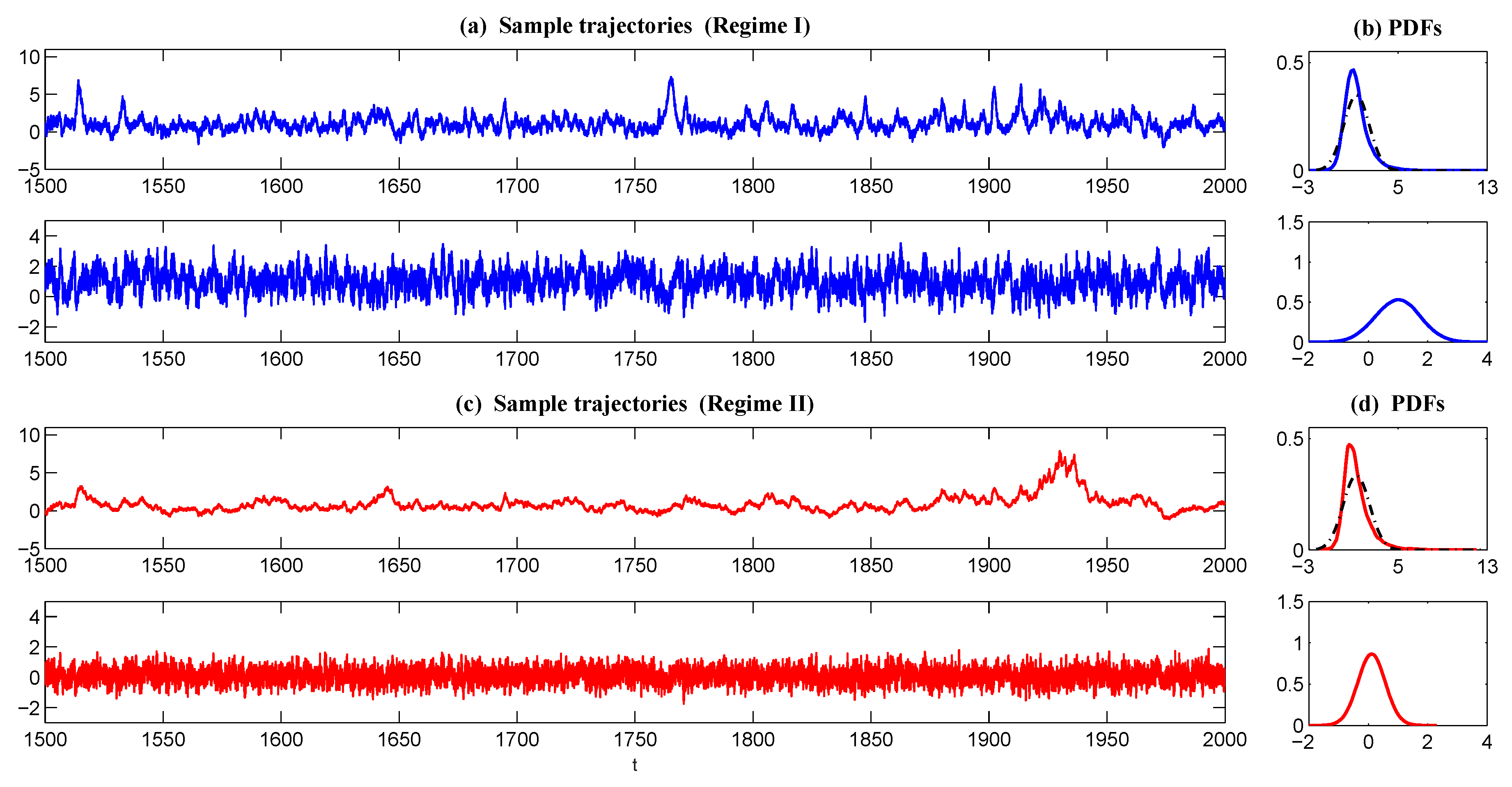
5.3. Intermittency with the Same Statistics, but Different Dynamical Behavior

Intermittency is an important topic in complex dynamical systems. They are typically characterized by strongly-non-Gaussian PDFs and extreme events. This subsection aims at quantifying the difference between different intermittencies using the information theory and emphasizing that simply using the non-Gaussian PDFs is not sufficient to distinguish different intermittent events.

The test example used here is a simplified version of the SPEKF model with only the stochastic damping,

$$\begin{array}{cc}\hfill \frac{du}{dt}& =-\gamma u+f+{\sigma }_u{\dot{W}}_u,\hfill \\ \hfill \frac{d\gamma }{dt}& =-d_{\gamma }(\gamma -\widehat{\gamma })+{\sigma }_{\gamma }{\dot{W}}_{\gamma }.\hfill \end{array}$$

(40)

From Section 5.1, it is clear that the stochastic damping $\gamma$ is able to trigger non-Gaussian features with intermittency and extreme events. However, focusing only on the equilibrium PDF may lead to a misleading conclusion for intermittent events since there are different mechanisms in generating these events. Consider the following two dynamical regimes,

$$\begin{array}{cc}\hfill \mathrm{Regime}\mathrm{I}:& f=1,\widehat{\gamma }=1,d_{\gamma }=2,{\sigma }_u=1,{\sigma }_{\gamma }=1.5,\hfill \\ \hfill \mathrm{Regime}\mathrm{II}:& f=0.1,\widehat{\gamma }=0.11,d_{\gamma }=6.8,{\sigma }_u=0.3,{\sigma }_{\gamma }=1.7.\hfill \end{array}$$

(41)

The corresponding trajectories and PDFs are shown in Figure 5. Both regimes contain extreme events, and the associated PDFs shown in Panels (b) and (d) are both skewed with a one-sided fat tail. As expected, the information distance computed from the relative entropy (1) between the two PDFs was tiny with $\mathcal{P}({\pi }^{\mathrm{I}}(\mathbf{u}),{\pi }^{\mathrm{II}}(\mathbf{u}))=0.0065$, where the superscripts I and II stand for Regimes I and II. However, this is not sufficient to make the conclusion that the two dynamical regimes have a similar dynamical behavior. In fact, the trajectories shown in Panels (a) and (c) clearly indicate the difference in these two regimes. In Regime I, the intermittency happened quite frequently, but has only a short duration. On the other hand, a less frequent occurrence, but longer duration time were found for the intermittent events in Regime II. These differences are mainly due to the mean damping $\widehat{\gamma }$ and the memory time of $\gamma$. In fact, the mean state of $\gamma$ in Regime I is relatively far from zero. Thus, only when negative $\gamma$ is triggered by the stochastic noise, the intermittency occurs. In Regime II, the mean value of $\gamma$ was nearly zero, which allowed the time series of u to stay in a nearly neural stable or weakly unstable status for a long time. Such a difference in the temporal patterns can be quantified by the spectrum density. In fact, the relative entropy between the two spectrum density functions in (9) was quite large with $\mathcal{P}(E^{\mathrm{I}}(\lambda ),E^{\mathrm{II}}(\lambda ))=0.8742$. Note that these different dynamical behavior of extreme events have been studied in [14]. The discussion here provides a quantitative way to assess the information distance in both temporal and statistical behavior.

6. Applying the GM FDT for Calculating the Linear Response in Strongly-Non-Gaussian Models

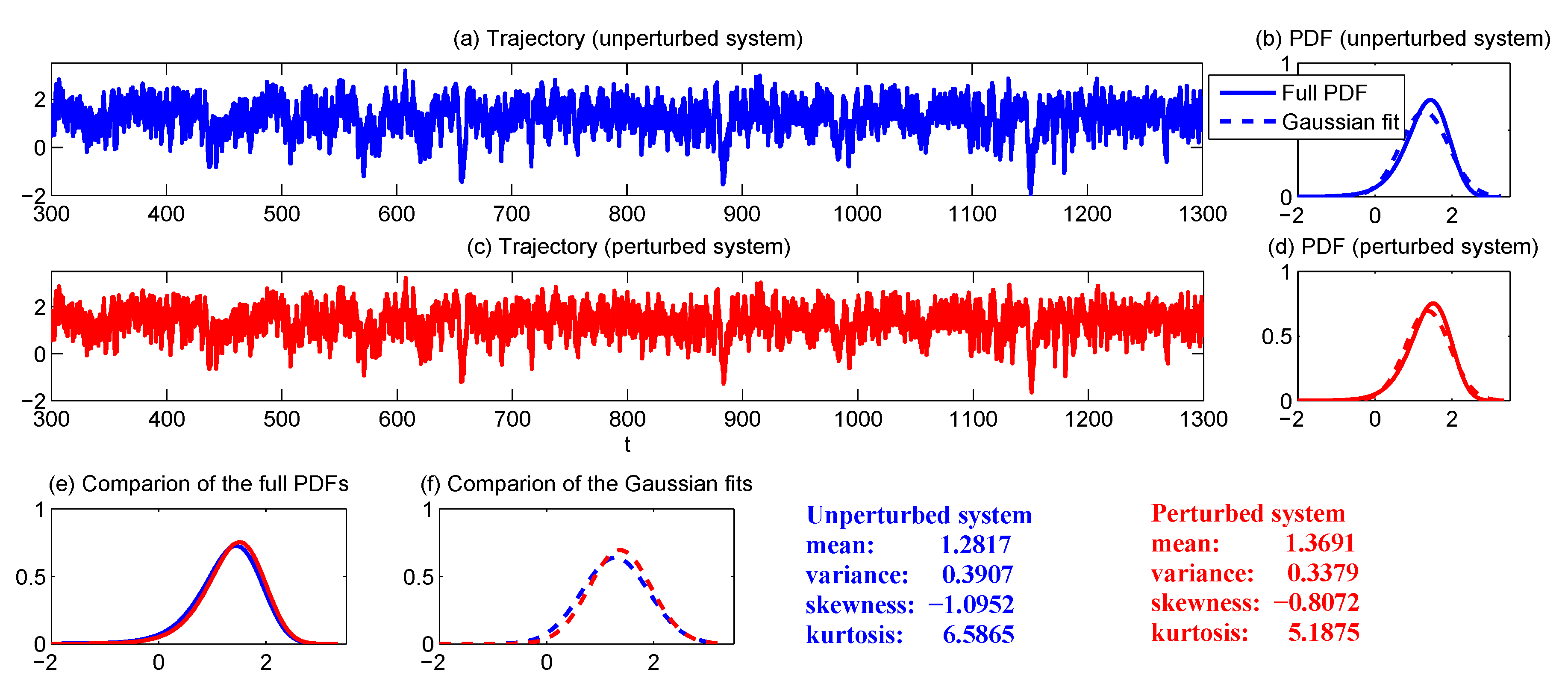
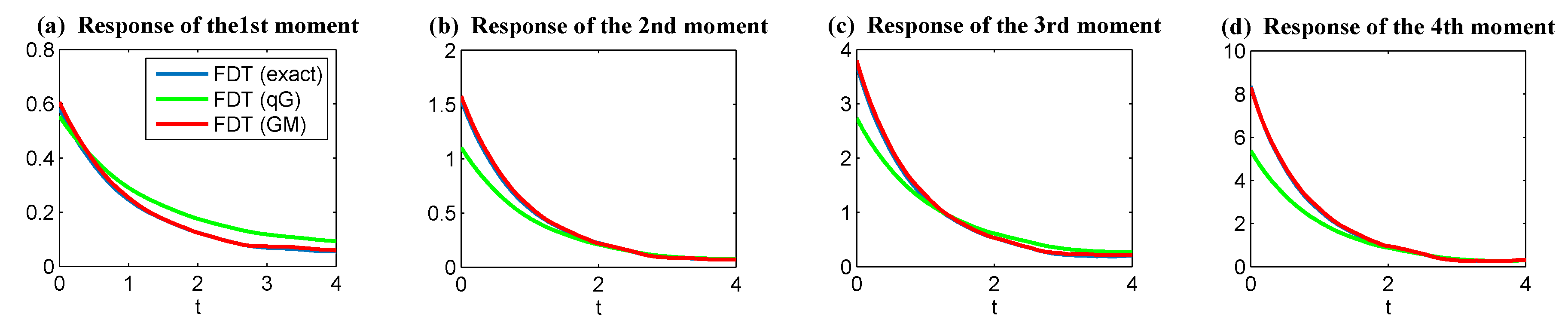
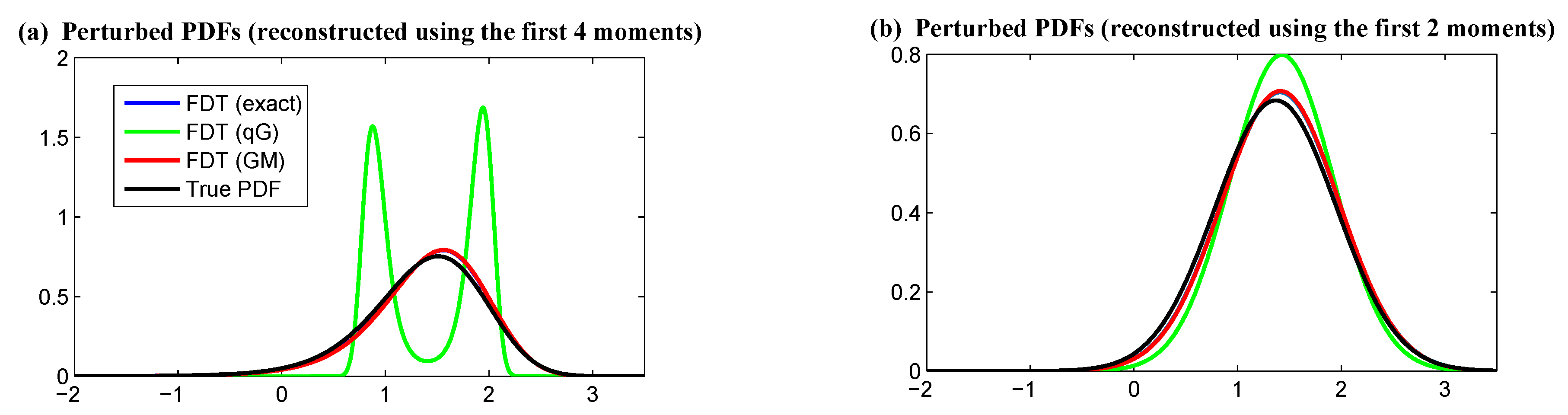
6.1. A Scalar Nonlinear Model

In the first example, the scalar nonlinear model for low frequency atmospheric variability with cubic nonlinearity and Correlated Additive and Multiplicative (CAM) noise [85,86] as used in Section 5.2 was studied,

$$\begin{array}{cc}\hfill \frac{du}{dt}& =F(u,t)+\sigma (u){\dot{W}}_u\hfill \\ & =(-c{u}^3+b{u}^2+au+f)+(A-Bu){\dot{W}}_C+{\sigma }_A{\dot{W}}_A,\hfill \end{array}$$

(42)

where $c>0,b,a,f,A,B$, and ${\sigma }_A$ are given constants and ${\dot{W}}_C$, ${\dot{W}}_A$ are independent white noise [53]. Due to the nonlinearity and the multiplicative noise, the statistics of (42) can be highly non-Gaussian. Therefore, it provides a testbed for understanding the skill of the linear response.

One desirable property of (42) is that the equilibrium PDF of (42) can be written down explicitly. Particularly, for the case of zero CAM noise, i.e., $A=B=0$, the PDF is given by:

$$\pi (u)=N_{0}exp\left(\frac{2}{{\sigma }_A^2}\left(fu+\frac{a}{2}{u}^2+\frac{b}{3}{u}^3-\frac{c}{4}{u}^4\right)\right),$$

(43)

where $N_0$ is a normalizing constant to make $\pi (u)$ integrate to one.

Note that since (42) is a scalar model, its PDF is recovered using the kernel estimation (29). The following parameter values are adopted for the system of the unperturbed state,

$$\begin{array}{c}a=-0.0222,b=-0.2,c=0.0494,f=0.6,\\ A=B=0,{\sigma }_A=0.7071.\end{array}$$

(44)

The perturbation is on the forcing term f with the perturbed amplitude:

$$\delta f=0.1\times f=0.06.$$

(45)

A trajectory and the associated PDF of the unperturbed PDF (Panels (a,b)), as well as those with the forcing perturbation (Panels (c,d)) are shown in Figure 6. For a fair comparison, the same random number seed was used in both experiments. It is clear that some extreme events appeared in the trajectory, and the PDF was skewed with an one-sided fat-tail, indicating that the regime, in the setup of (44), was strongly non-Gaussian. With the forcing perturbation in (45), the mean and variance increased and decreased, respectively. The skewness and kurtosis both decreased, which implies the perturbation reduced the non-Gaussian features.

In Figure 7, the linear response operator $R(t)$ in (24) for the response of the first four moments is shown. To obtain $p_{eq}$, three different methods were used: 1. the explicit expression given by (43), namely the exact FDT; 2. the computation from qG FDT (26), and 3. computation from GM FDT using $L=500$ samples (see Section 4.2). The linear response computed using these three $p_{eq}$s are represented in blue, red, and green curves in Figure 7. It is clear that since the Gaussian mixture provided an accurate recovery of the full non-Gaussian PDF, the linear response using the GM FDT led to results that were nearly the same as those from the FDT using the analytic PDF.

Finally, we compared the perturbed PDFs that were reconstructed by adding the response statistics to the unperturbed PDFs. Here, the perturbed PDFs correspond to the system state that has been transited to the new equilibrium state, which was achieved after a sufficiently long time. The difference between the perturbed and unperturbed PDFs was quantified by the relative entropy. The reference solution was given by the analytic Formula (43) with perturbed parameters (45), as shown in black in Figure 8. Other perturbed PDFs were obtained through the maximum entropy principle, a technique presented in Appendix B, which was applied to reconstruct PDFs upon the linear response correction from the first four (or two) moments being added. An interesting feature of this problem is that according to the analytic Formula (43) and the general recovered PDFs from the maximum entropy principle (A7), the full PDF of the nonlinear scalar model (42) without CAM noise is fully determined by the first four moments. Therefore, using four moments to recover the perturbed PDF is expected to give the full PDF, while using two moments for the recovery only gives a Gaussian approximation (see (A8)).

From Figure 8, it is clear that the reconstructed PDFs using the response of the moments calculated from the GM FDT (red) overlapped with the ones using those calculated from the exact FDT (blue). Note that this is not the true response since the linear response itself (24) represents only the leading order approximation (see (19) and (20)). Therefore, a small gap is seen between the black and the blue/red curves, which can be regarded as an intrinsic barrier due to the linearization in FDT, and it cannot be overcome by improving the accuracy of computing the $p_{eq}$ in the FDT. On the other hand, the reconstructed full PDF using the qG FDT (green), which is bimodal based on the maximum entropy principle, was very different from the truth. In fact, even the recovered Gaussian approximation (Panel (b)) from the qG FDT contained an obvious error, which indicates that the qG FDT cannot accurately capture the variance response in this case. See the error listed in

Table 2. Nonlinear scalar model. Errors in the perturbed PDFs reconstructed by the linear response compared with the true perturbed PDF. The error is given by the relative entropy (1).

	FDT (exact)	FDT (qG)	FDT (GM)
u (2 moments)	0.0034	0.0268	0.0040
u (4 moments)	0.0040	0.7524	0.0044

. The error was mainly due to the non-symmetry of the unperturbed PDF, where the qG FDT had no skill in including this information. On the other hand, the GM FDT was computationally efficient, and it was able to take into account non-Gaussian features in $p_{eq}$; thus, it outperformed qG FDT in the computation of the linear response.

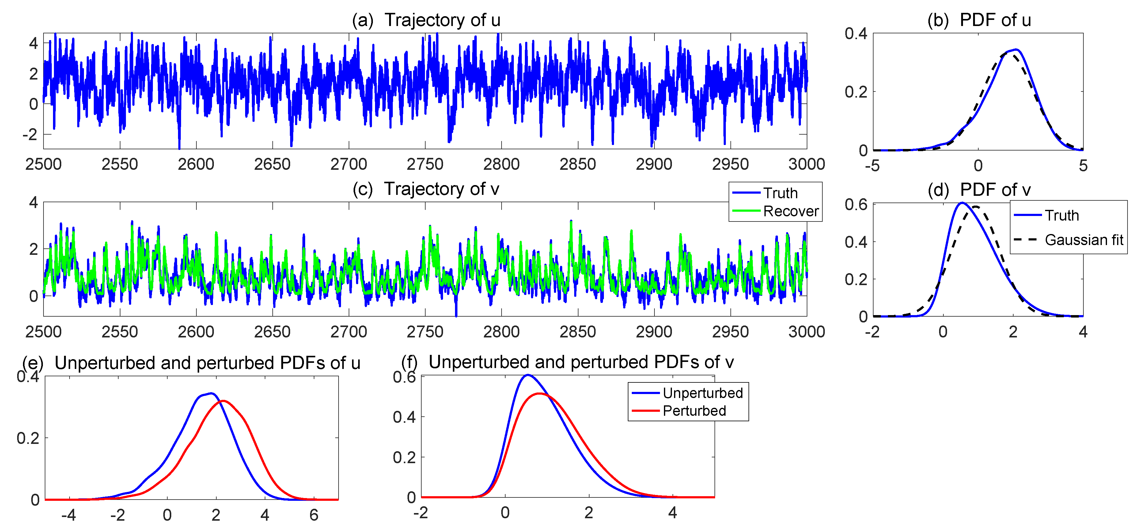
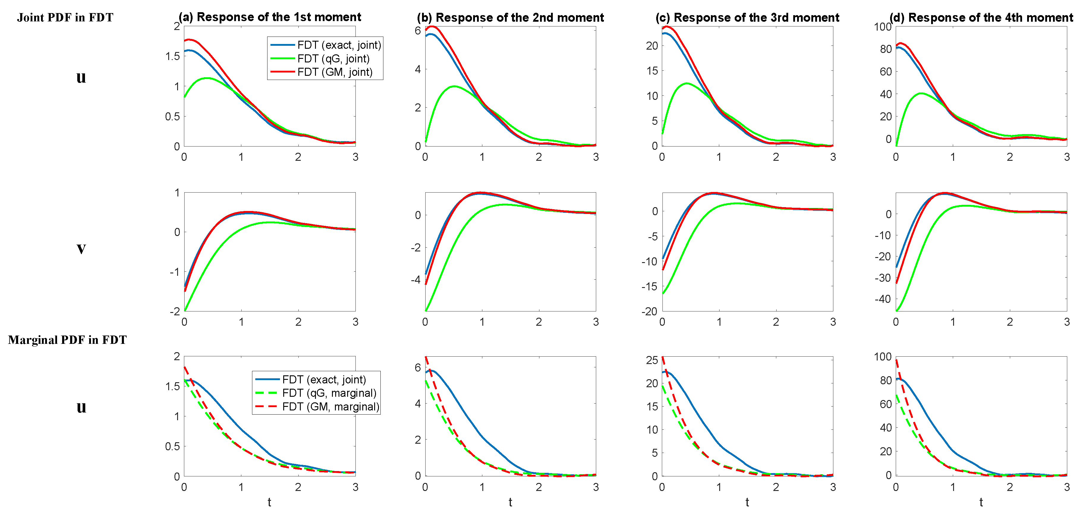
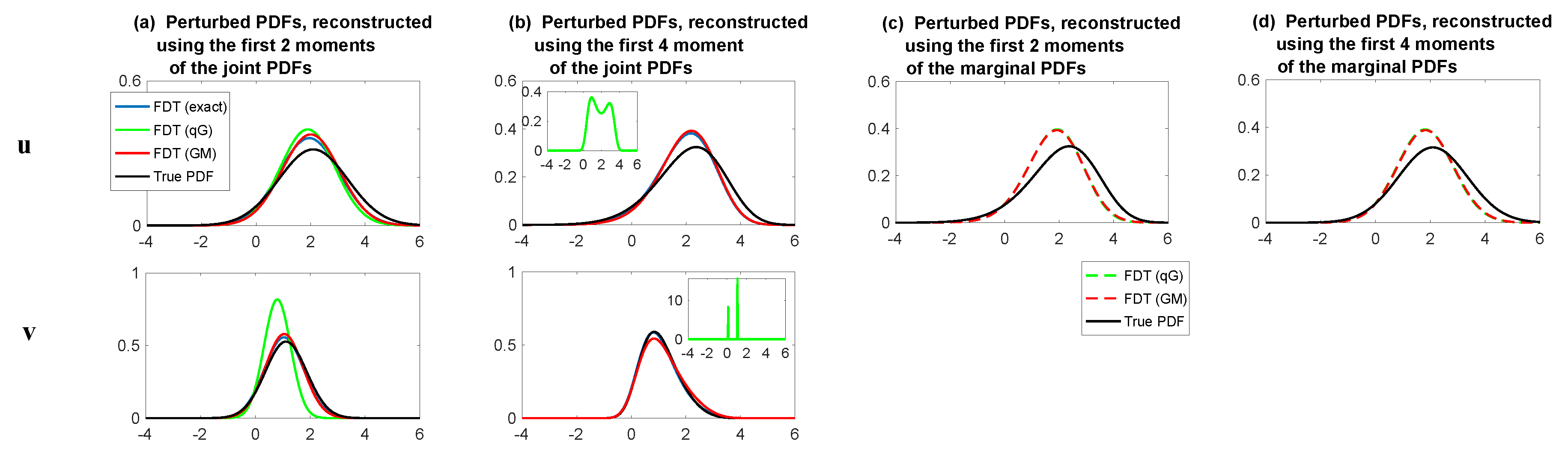
6.2. A Dyad Model with Energy-Conserving Nonlinearity

The second test example here involves a dyad model with energy-conserving nonlinearity:

$$\begin{array}{cc}\hfill \frac{du}{dt}& =(-d_{uu}+cv)u+F+{\sigma }_u{\dot{W}}_u,\hfill \\ \hfill \frac{dv}{dt}& =(-d_{vv}v+c{u}^2)+{\sigma }_v{\dot{W}}_v,\hfill \end{array}$$

(46)

where $c,d_{uu},d_{vv},{\sigma }_u,{\sigma }_v$, and F are given constants and ${\dot{W}}_u$ and ${\dot{W}}_v$ are independent white noise. In this nonlinear model, the total energy in the nonlinear terms is conserved, which is also known as the physical constraint [23,24]. This crucial property allows a systematical framework for model reduction, data assimilation, and prediction. Note that in most of the applications, u can be regarded as one of the large-scale resolved variables and is fully observed, while v is a small-scale variable containing unknown details. Given the observed trajectory of u, the variable v conditioned on the historical trajectory of u is conditional Gaussian. The hybrid strategy (30) was applied to solve the full non-Gaussian joint PDF of u and v.

The following parameters were adopted in the dyad model (46) for computing the unperturbed equilibrium states,

$$\begin{array}{c}{d}_{uu}=0.2,d_{vv}=1.5,\gamma =-0.4,\\ F=1,{\sigma }_u=1.5,{\sigma }_v=0.5.\end{array}$$

(47)

Sample trajectories of both u and v, as well as the associated PDFs are shown in Panels (a–d) (in blue color) of Figure 9. It is clear that both u and v were highly non-Gaussian with negative and positive skewness, respectively.

The perturbation was on both the nonlinear feedback coefficient $\gamma$ and the forcing F with:

$$\delta \gamma =-0.3\gamma =0.12,\delta F=0.3F=0.3.$$

(48)

The perturbed PDFs are shown in Panels (e) and (f) in red. The perturbation of the parameters changed the statistics of both u and v.

The first two rows of Figure 10 show the linear response operator $R(t)$ in (24) with the two components associated with u and v, respectively. Here, the linear responses were computed using the FDT Formula (24) with the two dimensional joint PDF $p(u,v)$. Similar to the results in the nonlinear scalar model, the response computed from the qG FDT (26) contained errors for both u and v. On the other hand, the GM FDT with $L=500$ matched very well with the exact FDT based on a large number of Monte Carlo samples (${10}^6$). Consequently, the recovered PDFs based on the GM FDT as shown in Columns (a) and (b) in Figure 11 were very similar to those based on the exact FDT. However, the PDFs recovered using the response from the qG FDT were far from the truth.

In many real applications, it is quite difficult to obtain the full information of the variables in the unresolved or unobserved scales. Therefore, marginal PDFs of the large-scale or resolved scale variables were utilized to compute the linear response. Obviously, this simplification saves the computational cost, but may lead to extra model error. Here, we assumed that only the response in u was of interest. We tested the skill of the response using FDT, where the $p_{eq}$ in the FDT was based only on the marginal PDF of u. Since the model (46) involves v in the first equation of the large-scale or resolved scale variable u, the trajectory of v was needed to compute the linear response operator. We assumed that we knew the form of the model (46) here. Then, we computed the conditioned mean of v via data assimilation, using that as the recovered trajectory of v. Note that the conditional mean of v can be compute from the closed form (A1a), as shown in Appendix A, and therefore, there was no extra numerical error here. The recovered trajectory of v is shown in Figure 9 (Panels (c) and (d) in green).

The linear response operators are shown in the third row of Figure 10, and the recovered PDFs are shown in Panels (c) and (d) in Figure 11. Using the marginal PDF in the GM FDT only resulted in slightly worse results compared with those using the joint PDF. This indicates some potentials for a further simplification in computing the linear response. An interesting phenomenon was that the qG FDT with the marginal PDF became skillful. See Panels (c) and (d) in Figure 11 and

Table 3. Dyad model. Errors in the perturbed PDFs reconstructed by the linear response compared with the true perturbed PDF. The error is given by the relative entropy (1).

	FDT (exact; joint)	FDT (qG; joint)	FDT (GM; joint)	FDT (qG; marginal)	FDT (GM; marginal)
u (2 moments)	0.0241	0.0596	0.0312	0.0659	0.0601
v (2 moments)	0.0074	0.2340	0.0121
u (4 moments)	0.0346	0.1696	0.0379	0.0823	0.0752
v (4 moments)	0.0061	2.9144	0.0093

. A possible explanation is that the largest error source came from the Gaussian approximation of v in computing the FDT. A biased PDF of v may provide a worse result than simply using the marginal PDF of u in computing the FDT. In fact, if v is regarded as a stochastic parameterization that provides the key mechanisms for the non-Gaussian behavior of u, then these results imply that a suitable stochastic parameterization of the unresolved variables is extremely important in the linear response, especially considering that perfect models cannot always be available in practice.

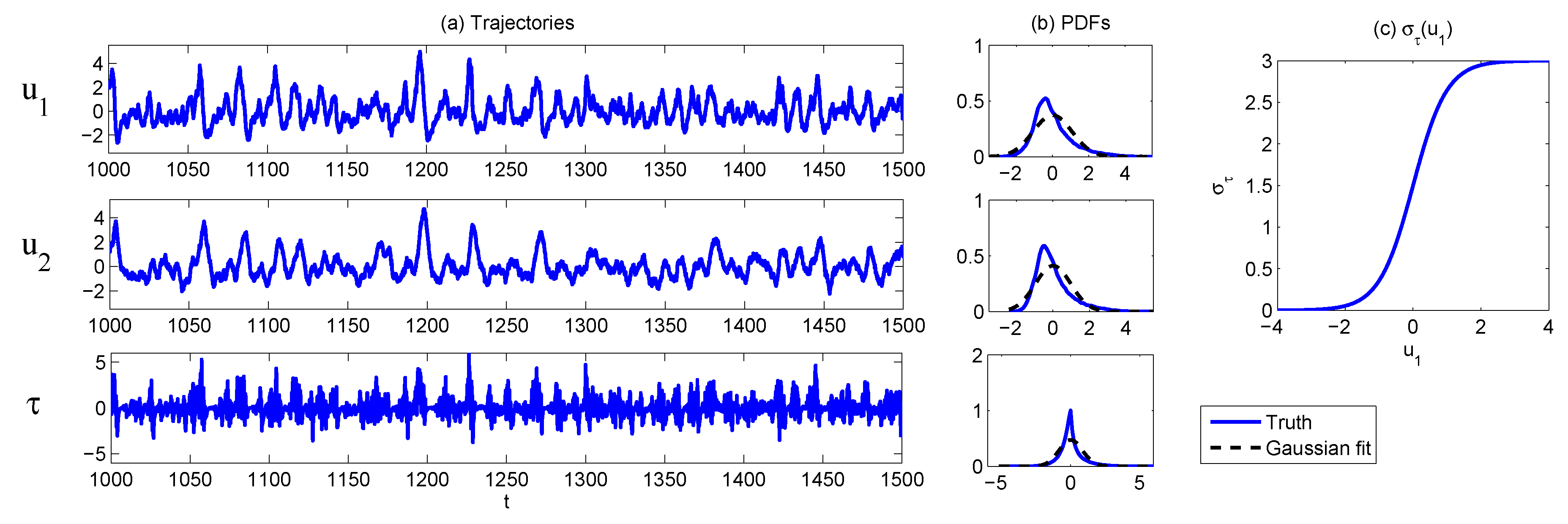
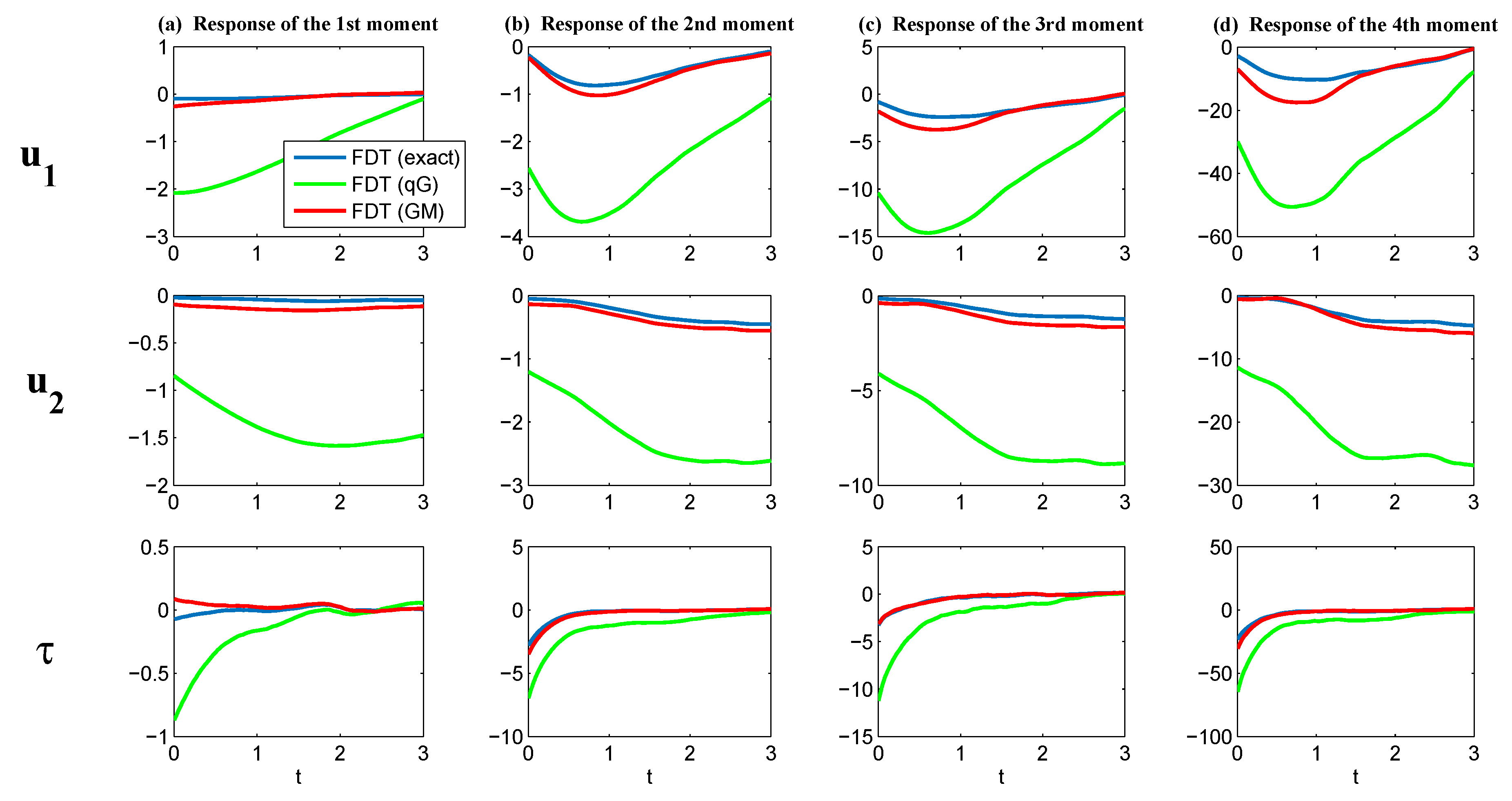
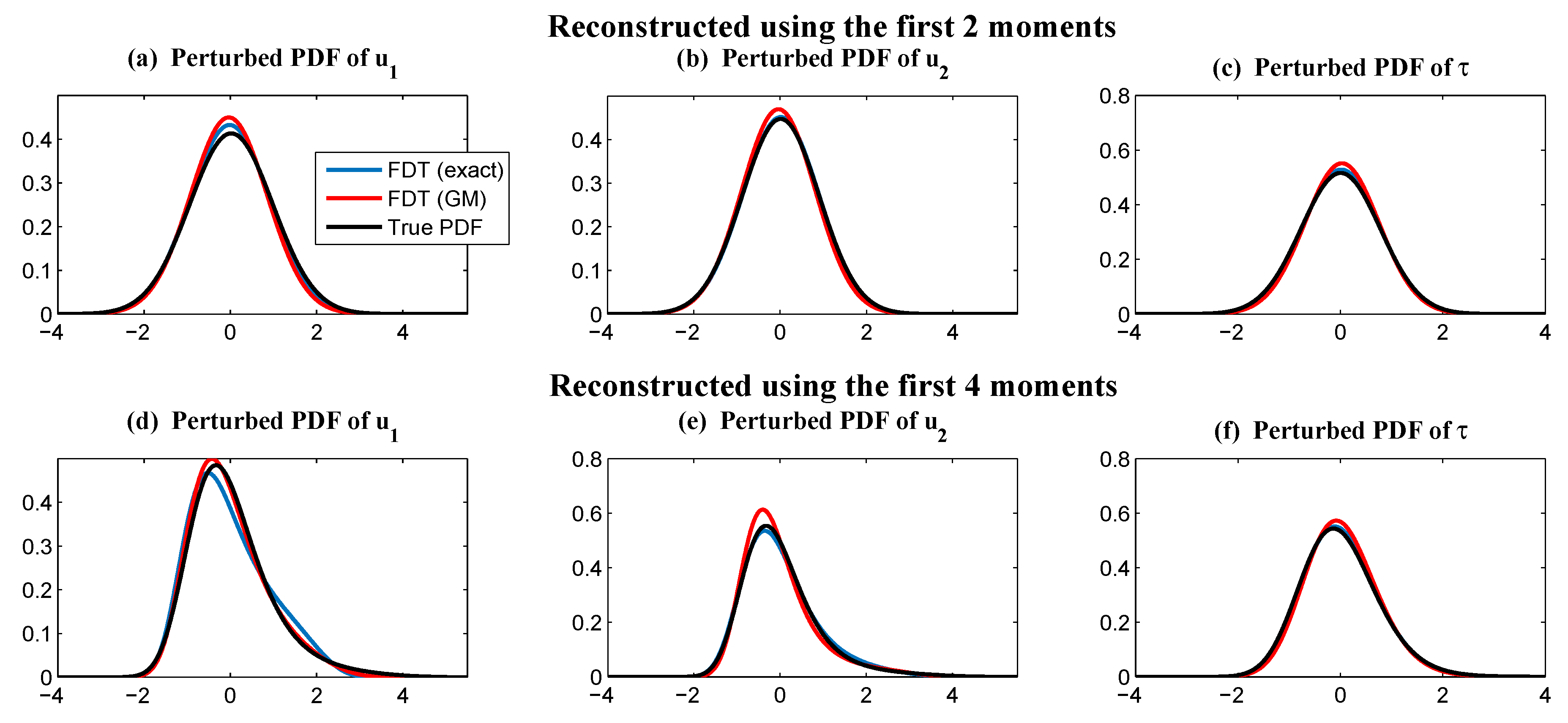
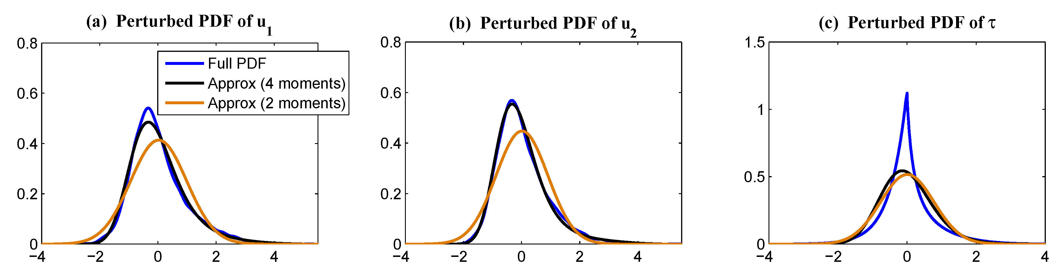
6.3. A Slow-Fast Triad Model with Potential Application to the Study of the El Niño-Southern Oscillation

Now, we consider a simple triad model with multiscale linear structure and multiplicative noise,

$$\begin{array}{cc}\hfill \frac{d{u}_1}{dt}& =(-d_u{u}_1-w_u{u}_2+\tau )+{\sigma }_{u_1}{\dot{W}}_{u_1}\hfill \\ \hfill \frac{d{u}_2}{dt}& =(-d_u{u}_2+w_u{u}_1)+{\sigma }_{u_2}d{\dot{W}}_{u_1}\hfill \\ \hfill \frac{d\tau }{dt}& =-d_{\tau }\tau +{\sigma }_{\tau }(u_1){\dot{W}}_{\tau },\hfill \end{array}$$

(49)

where $u_1$ and $u_2$ are a pair of slow variables that form an oscillation, and they can usually be resolved; while $\tau$ lies in the fast time scale; and its random amplitude depends on the state variable $u_1$. This model belongs to the conditional Gaussian framework, and it allows us to study the effect of linear response in the presence of hidden multiplicative noise. This model can be derived from the leading modes of an intermediate model [88] and thus serves as a toy model for the El Niño Southern Oscillation (ENSO) that preserves the very basic structures of physics. In fact, if $u_1$ and $u_2$ are thought as the Western Pacific thermocline depth (or heat content) and the Eastern Pacific sea surface temperature, then $\tau$ can be regarded as the zonal wind bursts in the Western Pacific. We choose the following parameters:

$$d_u=0.2,d_{\tau }=2,\omega =0.4,{\sigma }_{u_1}=0.3,{\sigma }_{u_2}=0.3.$$

(50)

Note that in (50), the memory (or damping) time of $\tau$ (wind bursts) is 10-times faster than that of $u_1,u_2$ (SST and thermocline), reflecting the correct ratio in physics (roughly one month vs. one year). The state-dependent noise coefficient in the third equation of (49) was chosen to be:

$${\sigma }_{\tau }(u_1)=1.5\left(tanh(u_1)+1\right),$$

(51)

which is shown in Panel (c) of Figure 12. This relation reflects the fact that the increases of the heat content in the Western Pacific will lead to more active wind bursts [89,90]. With these parameters, the model simulation is shown in Panel (a) of Figure 12, and the associated PDFs are shown in Panel (b). Clearly, the trajectories of $u_1$ and $u_2$ formed an oscillator, where the positive phase had a larger amplitude, but the negative phase had a longer duration for each event. These are consistent with the observed ENSO features found in various ENSO indices [91,92]. In addition, the PDFs of $u_1$ and $u_2$ are highly non-Gaussian with extreme events in the positive direction that correspond to strong El Niños.

Now, we perturb the system by putting:

$$\delta d_{\tau }=-0.2d_{\tau }=-0.4,$$

(52)

which means the memory time of $\tau$ is increased and, meanwhile, the strength of the wind bursts is enhanced. Physically, this can be regarded as the increase of the Madden-Julian oscillation or the monsoon activities in the Western Pacific that modify the ENSO behavior [93,94,95]. A direct consequence is that the variance of $u_1$ and $u_2$ becomes larger, increasing the occurrence of strong ENSO events.

Now, we test various FDT methods in computing the linear response. Figure 13 shows the linear response operator $\mathbf{R}(t)$ for both the slow variables $u_1,u_2$ and the fast variable $\tau$. In this strongly-non-Gaussian model, the qG FDT completely failed, while the GM FDT with $L=500$ was extremely skillful. Note that the blue curves in Figure 13 show the linear response computed from the exact FDT, with the PDF constructed using ${10}^6$ Monte Carlo samples. Figure 14 shows that the reconstructed PDFs based on the GM FDT were almost the same as the perfect perturbed PDFs from the linear response. See also the error computed via relative entropy between various reconstructed PDFs with the one computed directly from Monte Carlo in

Table 4. Triad model. Errors in the perturbed PDFs reconstructed by the linear response compared with the true perturbed PDF. The error is given by the relative entropy (1).

	FDT (exact)	FDT (qG)	FDT (GM)
$u_1$ (2 moments)	0.0028	4.4909	0.0086
$u_2$ (2 moments)	0.0001	4.3432	0.0038
$\tau$ (2 moments)	0.0006	3.5908	0.0047
$u_1$ (4 moments)	0.0230	2.1175	0.0107
$u_2$ (4 moments)	0.0047	2.3717	0.0096
$\tau$ (4 moments)	0.0006	2.0072	0.0050

. Note that, despite that the reconstructed PDFs of $u_1$ and $u_2$ using the leading four moments were nearly the same as the full PDFs, the gap between the reconstructed PDF of $\tau$ was quite big in this extremely non-Gaussian case, even when there were four moments that were being adjusted. See Figure 15. This reflects some fundamental difficulties in capturing the statistical response in the wind bursts for the study of ENSO, especially considering that the higher order moments are numerically challenging to capture.

7. Conclusions

In this article, information theory was applied to understand the complex turbulent dynamical systems with nonlinear and non-Gaussian features. In the first part of this article, an information-theoretic framework was developed that involved the quantification of model error in both the equilibrium statistics and the spectrum density associated with the temporal autocorrelation function via relative entropy. This information-theoretic framework was applied to the study of the model reduction, stochastic parameterizations, and intermittent events. In the second part of this article, an efficient method of calculating the statistical response was proposed. This new method involves a Gaussian Mixture (GM) FDT that takes into account non-Gaussian information in the computation of the linear response. Several simple, but illustrative examples in light of information measurement showed that this GM FDT had significant advantages over the quasi-Gaussian (qG) FDT, especially in the regimes that present strongly non-Gaussian features.

One important future topic is to study the effect of various errors in the response theory systematically. The first error appeared in applying the FDT due to the linearization of the evolution of the statistics. This is an intrinsic barrier in the FDT methods. Another error came from computing the unperturbed PDF $p_{eq}$ in the linear response. Experiments showed that such error could be significantly reduced and even eliminated by GM FDT. One other potential error appeared if marginal PDFs were adopted in computing the FDT. It is interesting to investigate and compare, especially in high dimensional systems, the skill of the FDT utilizing marginal, but non-Gaussian, PDFs and joint, but Gaussian, PDFs.

References

1. Majda, A.J. Introduction to Turbulent Dynamical Systems in Complex Systems; Springer: New York, NY, USA, 2016. [Google Scholar]
2. Majda, A.; Wang, X. Nonlinear Dynamics and Statistical Theories for Basic Geophysical Flows; Cambridge University Press: Cambridge, UK, 2006. [Google Scholar]
3. Strogatz, S.H. Nonlinear Dynamics and Chaos: With Applications to Physics, Biology, Chemistry, and Engineering; CRC Press: Boca Raton, FL, USA, 2018. [Google Scholar]
4. Baleanu, D.; Machado, J.A.T.; Luo, A.C. Fractional Dynamics and Control; Springer Science & Business Media: New York, NY, USA, 2011. [Google Scholar]
5. Deisboeck, T.; Kresh, J.Y. Complex Systems Science in Biomedicine; Springer Science & Business Media: New York, NY, USA, 2007. [Google Scholar]
6. Stelling, J.; Kremling, A.; Ginkel, M.; Bettenbrock, K.; Gilles, E. Foundations of Systems Biology; MIT Press: Cambridge, MA, USA, 2001. [Google Scholar]
7. Sheard, S.A.; Mostashari, A. Principles of complex systems for systems engineering. Syst. Eng. 2009, 12, 295–311. [Google Scholar] [CrossRef]
8. Wilcox, D.C. Multiscale model for turbulent flows. AIAA J. 1988, 26, 1311–1320. [Google Scholar] [CrossRef]
9. Majda, A.J.; Gershgorin, B. Quantifying uncertainty in climate change science through empirical information theory. Proc. Natl. Acad. Sci. USA 2010, 107, 14958–14963. [Google Scholar] [CrossRef] [Green Version]
10. Majda, A.J.; Gershgorin, B. Improving model fidelity and sensitivity for complex systems through empirical information theory. Proc. Natl. Acad. Sci. USA 2011, 108, 10044–10049. [Google Scholar] [CrossRef] [Green Version]
11. Majda, A.J.; Gershgorin, B. Link between statistical equilibrium fidelity and forecasting skill for complex systems with model error. Proc. Natl. Acad. Sci. USA 2011, 108, 12599–12604. [Google Scholar] [CrossRef] [Green Version]
12. Gershgorin, B.; Majda, A.J. Quantifying uncertainty for climate change and long-range forecasting scenarios with model errors. part I: Gaussian models. J. Clim. 2012, 25, 4523–4548. [Google Scholar] [CrossRef]
13. Majda, A.J.; Branicki, M. Lessons in uncertainty quantification for turbulent dynamical systems. Discret. Contin. Dyn. Syst.-A 2012, 32, 3133–3221. [Google Scholar] [Green Version]
14. Branicki, M.; Majda, A.J. Quantifying uncertainty for predictions with model error in non-Gaussian systems with intermittency. Nonlinearity 2012, 25, 2543. [Google Scholar] [CrossRef]
15. Branicki, M.; Majda, A. Quantifying Bayesian filter performance for turbulent dynamical systems through information theory. Commun. Math. Sci 2014, 12, 901–978. [Google Scholar] [CrossRef] [Green Version]
16. Kleeman, R. Information theory and dynamical system predictability. Entropy 2011, 13, 612–649. [Google Scholar] [CrossRef]
17. Kleeman, R. Measuring dynamical prediction utility using relative entropy. J. Atmos. Sci. 2002, 59, 2057–2072. [Google Scholar] [CrossRef]
18. Majda, A.; Kleeman, R.; Cai, D. A mathematical framework for quantifying predictability through relative entropy. Methods Appl. Anal. 2002, 9, 425–444. [Google Scholar]
19. Majda, A.J.; Qi, D. Strategies for reduced-order models for predicting the statistical responses and uncertainty quantification in complex turbulent dynamical systems. SIAM Rev. 2018, in press. [Google Scholar] [CrossRef]
20. Sapsis, T.P.; Majda, A.J. A statistically accurate modified quasilinear Gaussian closure for uncertainty quantification in turbulent dynamical systems. Phys. D Nonlinear Phenom. 2013, 252, 34–45. [Google Scholar] [CrossRef]
21. Sapsis, T.P.; Majda, A.J. Statistically accurate low-order models for uncertainty quantification in turbulent dynamical systems. Proc. Natl. Acad. Sci. USA 2013, 110, 13705–13710. [Google Scholar] [CrossRef] [Green Version]
22. Chen, N.; Majda, A.J.; Giannakis, D. Predicting the cloud patterns of the Madden-Julian Oscillation through a low-order nonlinear stochastic model. Geophys. Res. Lett. 2014, 41, 5612–5619. [Google Scholar] [CrossRef] [Green Version]
23. Harlim, J.; Mahdi, A.; Majda, A.J. An ensemble Kalman filter for statistical estimation of physics constrained nonlinear regression models. J. Comput. Phys. 2014, 257, 782–812. [Google Scholar] [CrossRef]
24. Majda, A.J.; Harlim, J. Physics constrained nonlinear regression models for time series. Nonlinearity 2012, 26, 201. [Google Scholar] [CrossRef]
25. Qi, D.; Majda, A.J. Predicting fat-tailed intermittent probability distributions in passive scalar turbulence with imperfect models through empirical information theory. Commun. Math. Sci. 2016, 14, 1687–1722. [Google Scholar] [CrossRef]
26. Qi, D.; Majda, A.J. Low-dimensional reduced-order models for statistical response and uncertainty quantification: Two-layer baroclinic turbulence. J. Atmos. Sci. 2016, 73, 4609–4639. [Google Scholar] [CrossRef]
27. Majda, A.; Chen, N. Model error, information barriers, state estimation and prediction in complex multiscale systems. Entropy 2018, 20, 644. [Google Scholar] [CrossRef]
28. Marconi, U.M.B.; Puglisi, A.; Rondoni, L.; Vulpiani, A. Fluctuation–dissipation: Response theory in statistical physics. Phys. Rep. 2008, 461, 111–195. [Google Scholar] [CrossRef] [Green Version]
29. Leith, C. Climate response and fluctuation dissipation. J. Atmos. Sci. 1975, 32, 2022–2026. [Google Scholar] [CrossRef]
30. Majda, A.; Abramov, R.V.; Grote, M.J. Information Theory and Stochastics for Multiscale Nonlinear Systems; American Mathematical Society: Providence, RI, USA, 2005; Volume 25. [Google Scholar]
31. Majda, A.J.; Gershgorin, B.; Yuan, Y. Low-frequency climate response and fluctuation–dissipation theorems: Theory and practice. J. Atmos. Sci. 2010, 67, 1186–1201. [Google Scholar] [CrossRef]
32. Gershgorin, B.; Majda, A.J. A test model for fluctuation–dissipation theorems with time-periodic statistics. Phys. D Nonlinear Phenom. 2010, 239, 1741–1757. [Google Scholar] [CrossRef]
33. Chen, N.; Majda, A.J. Beating the curse of dimension with accurate statistics for the Fokker–Planck equation in complex turbulent systems. Proc. Natl. Acad. Sci. USA 2017, 114, 12864–12869. [Google Scholar] [CrossRef] [Green Version]
34. Chen, N.; Majda, A.J. Efficient statistically accurate algorithms for the Fokker–Planck equation in large dimensions. J. Comput. Phys. 2018, 354, 242–268. [Google Scholar] [CrossRef] [Green Version]
35. Kullback, S.; Leibler, R.A. On information and sufficiency. Ann. Math. Stat. 1951, 22, 79–86. [Google Scholar] [CrossRef]
36. Kullback, S. Letter to the editor: The Kullback–Leibler distance. Am. Stat. 1987, 41, 338–341. [Google Scholar]
37. Kullback, S. Statistics and Information Theory; John & Wiley Sons: New York, NY, USA, 1959. [Google Scholar]
38. Branstator, G.; Teng, H. Two limits of initial-value decadal predictability in a CGCM. J. Clim. 2010, 23, 6292–6311. [Google Scholar] [CrossRef]
39. DelSole, T. Predictability and information theory. Part I: Measures of predictability. J. Atmos. Sci. 2004, 61, 2425–2440. [Google Scholar] [CrossRef]
40. DelSole, T. Predictability and information theory. Part II: Imperfect forecasts. J. Atmos. Sci. 2005, 62, 3368–3381. [Google Scholar] [CrossRef]
41. Giannakis, D.; Majda, A.J. Quantifying the predictive skill in long-range forecasting. Part II: Model error in coarse-grained Markov models with application to ocean-circulation regimes. J. Clim. 2012, 25, 1814–1826. [Google Scholar] [CrossRef]
42. Teng, H.; Branstator, G. Initial-value predictability of prominent modes of North Pacific subsurface temperature in a CGCM. Clim. Dyn. 2011, 36, 1813–1834. [Google Scholar] [CrossRef]
43. Yaglom, A.M. An Introduction to the Theory of Stationary Random Functions; Courier Corporation: New York, NY, USA, 2004. [Google Scholar]
44. McGraw, M.C.; Barnes, E.A. Seasonal Sensitivity of the Eddy-Driven Jet to Tropospheric Heating in an Idealized AGCM. J. Clim. 2016, 29, 5223–5240. [Google Scholar] [CrossRef]
45. Majda, A.; Wang, X. Linear response theory for statistical ensembles in complex systems with time-periodic forcing. Commun. Math. Sci. 2010, 8, 145–172. [Google Scholar] [CrossRef]
46. Gritsun, A.; Branstator, G. Climate response using a three-dimensional operator based on the fluctuation–dissipation theorem. J. Atmos. Sci. 2007, 64, 2558–2575. [Google Scholar] [CrossRef]
47. Gritsun, A.; Branstator, G.; Majda, A. Climate response of linear and quadratic functionals using the fluctuation–dissipation theorem. J. Atmos. Sci. 2008, 65, 2824–2841. [Google Scholar] [CrossRef]
48. Fuchs, D.; Sherwood, S.; Hernandez, D. An Exploration of Multivariate Fluctuation Dissipation Operators and Their Response to Sea Surface Temperature Perturbations. J. Atmos. Sci. 2015, 72, 472–486. [Google Scholar] [CrossRef] [Green Version]
49. Lutsko, N.J.; Held, I.M.; Zurita-Gotor, P. Applying the Fluctuation-Dissipation Theorem to a Two-Layer Model of Quasigeostrophic Turbulence. J. Atmos. Sci. 2015, 72, 3161–3177. [Google Scholar] [CrossRef]
50. Hassanzadeh, P.; Kuang, Z. The Linear Response Function of an Idealized Atmosphere. Part II: Implications for the Practical Use of the Fluctuation-Dissipation Theorem and the Role of Operator’s Nonnormality. J. Atmos. Sci. 2016, 73, 3441–3452. [Google Scholar] [CrossRef]
51. Gritsun, A.; Lucarini, V. Fluctuations, response, and resonances in a simple atmospheric model. Phys. D Nonlinear Phenom. 2017, 349, 62–76. [Google Scholar] [CrossRef] [Green Version]
52. Nicolis, C.; Nicolis, G. The Fluctuation-Dissipation Theorem Revisited: Beyond the Gaussian Approximation. J. Atmos. Sci. 2015, 72, 2642–2656. [Google Scholar] [CrossRef]
53. Gardiner, C.W. Handbook of Stochastic Methods for Physics, Chemistry and the Natural Sciences, Volume 13 of Springer Series in Synergetics; Springer: Berlin/Heidelberg, Germany, 2004. [Google Scholar]
54. Risken, H. Fokker-planck equation. In The Fokker–Planck Equation; Springer: Berlin/Heidelberg, Germany, 1996; pp. 63–95. [Google Scholar]
55. Daum, F. Nonlinear filters: Beyond the Kalman filter. IEEE Aerosp. Electron. Syst. Mag. 2005, 20, 57–69. [Google Scholar] [CrossRef]
56. Sjöberg, P.; Lötstedt, P.; Elf, J. Fokker–Planck approximation of the master equation in molecular biology. Comput. Vis. Sci. 2009, 12, 37–50. [Google Scholar] [CrossRef]
57. Majda, A.J.; Qi, D. Improving prediction skill of imperfect turbulent models through statistical response and information theory. J. Nonlinear Sci. 2016, 26, 233–285. [Google Scholar] [CrossRef]
58. Proistosescu, C.; Rhines, A.; Huybers, P. Identification and interpretation of nonnormality in atmospheric time series. Geophys. Res. Lett. 2016, 43, 5425–5434. [Google Scholar] [CrossRef] [Green Version]
59. Loikith, P.C.; Neelin, J.D. Short-tailed temperature distributions over North America and implications for future changes in extremes. Geophys. Res. Lett. 2015, 42, 8577–8585. [Google Scholar] [CrossRef]
60. Chen, N.; Majda, A.J.; Tong, X.T. Rigorous Analysis for Efficient Statistically Accurate Algorithms for Solving Fokker–Planck Equations in Large Dimensions. SIAM/ASA J. Uncertain. Quantif. 2018, 6, 1198–1223. [Google Scholar] [CrossRef]
61. Chen, N.; Majda, A.J. Filtering nonlinear turbulent dynamical systems through conditional Gaussian statistics. Mon. Weather Rev. 2016, 144, 4885–4917. [Google Scholar] [CrossRef]
62. Chen, N.; Majda, A. Conditional Gaussian Systems for Multiscale Nonlinear Stochastic Systems: Prediction, State Estimation and Uncertainty Quantification. Entropy 2018, 20, 509. [Google Scholar] [CrossRef]
63. Liptser, R.S.; Shiryaev, A.N. Statistics of Random Processes II: Applications; Springer: Berlin/Heidelberg, Germany, 2001; pp. 177–218. [Google Scholar]
64. Chen, N.; Majda, A.J. Predicting the real-time multivariate Madden–Julian oscillation index through a low-order nonlinear stochastic model. Mon. Weather Rev. 2015, 143, 2148–2169. [Google Scholar] [CrossRef]
65. Chen, N.; Majda, A.J. Predicting the Cloud Patterns for the Boreal Summer Intraseasonal Oscillation Through a Low-Order Stochastic Model. Math. Clim. Weather Forecast. 2015, 1, 1–20. [Google Scholar] [CrossRef]
66. Chen, N.; Majda, A.J.; Sabeerali, C.; Ajayamohan, R. Predicting Monsoon Intraseasonal Precipitation using a Low-Order Nonlinear Stochastic Model. J. Clim. 2018, 31, 4403–4427. [Google Scholar] [CrossRef]
67. Chen, N.; Majda, A.J. Filtering the stochastic skeleton model for the Madden–Julian oscillation. Mon. Weather Rev. 2016, 144, 501–527. [Google Scholar] [CrossRef]
68. Chen, N.; Majda, A.J.; Tong, X.T. Information barriers for noisy Lagrangian tracers in filtering random incompressible flows. Nonlinearity 2014, 27, 2133. [Google Scholar] [CrossRef]
69. Chen, N.; Majda, A.J.; Tong, X.T. Noisy Lagrangian tracers for filtering random rotating compressible flows. J. Nonlinear Sci. 2015, 25, 451–488. [Google Scholar] [CrossRef]
70. Chen, N.; Majda, A.J. Model error in filtering random compressible flows utilizing noisy Lagrangian tracers. Mon. Weather Rev. 2016, 144, 4037–4061. [Google Scholar] [CrossRef]
71. Branicki, M.; Majda, A.J. Dynamic stochastic superresolution of sparsely observed turbulent systems. J. Comput. Phys. 2013, 241, 333–363. [Google Scholar] [CrossRef]
72. Keating, S.R.; Majda, A.J.; Smith, K.S. New methods for estimating ocean eddy heat transport using satellite altimetry. Mon. Weather Rev. 2012, 140, 1703–1722. [Google Scholar] [CrossRef]
73. Majda, A.J.; Grooms, I. New perspectives on super-parameterization for geophysical turbulence. J. Comput. Phys. 2014, 271, 60–77. [Google Scholar] [CrossRef]
74. Majda, A.J.; Qi, D.; Sapsis, T.P. Blended particle filters for large-dimensional chaotic dynamical systems. Proc. Natl. Acad. Sci. USA 2014, 111, 7511–7516. [Google Scholar] [CrossRef] [Green Version]
75. Botev, Z.I.; Grotowski, J.F.; Kroese, D.P. Kernel density estimation via diffusion. Ann. Stat. 2010, 38, 2916–2957. [Google Scholar] [CrossRef] [Green Version]
76. Cooper, F.C.; Haynes, P.H. Climate Sensitivity via a Nonparametric Fluctuation–Dissipation Theorem. J. Atmos. Sci. 2011, 68, 937–953. [Google Scholar] [CrossRef]
77. Crommelin, D.; Majda, A. Strategies for model reduction: Comparing different optimal bases. J. Atmos. Sci. 2004, 61, 2206–2217. [Google Scholar] [CrossRef]
78. Mezić, I. Spectral properties of dynamical systems, model reduction and decompositions. Nonlinear Dyn. 2005, 41, 309–325. [Google Scholar] [CrossRef]
79. Gouda, M.; Danaher, S.; Underwood, C. Building thermal model reduction using nonlinear constrained optimization. Build. Environ. 2002, 37, 1255–1265. [Google Scholar] [CrossRef]
80. Majda, A.J.; Harlim, J.; Gershgorin, B. Mathematical strategies for filtering turbulent dynamical systems. Discret. Contin. Dyn. Syst. 2010, 27, 441–486. [Google Scholar] [CrossRef] [Green Version]
81. Plant, R.; Craig, G.C. A stochastic parameterization for deep convection based on equilibrium statistics. J. Atmos. Sci. 2008, 65, 87–105. [Google Scholar] [CrossRef]
82. Lin, J.W.B.; Neelin, J.D. Influence of a stochastic moist convective parameterization on tropical climate variability. Geophys. Res. Lett. 2000, 27, 3691–3694. [Google Scholar] [CrossRef] [Green Version]
83. Frenkel, Y.; Majda, A.J.; Khouider, B. Using the stochastic multicloud model to improve tropical convective parameterization: A paradigm example. J. Atmos. Sci. 2012, 69, 1080–1105. [Google Scholar] [CrossRef]
84. Jung, T.; Palmer, T.; Shutts, G. Influence of a stochastic parameterization on the frequency of occurrence of North Pacific weather regimes in the ECMWF model. Geophys. Res. Lett. 2005, 32. [Google Scholar] [CrossRef] [Green Version]
85. Majda, A.J.; Abramov, R.; Gershgorin, B. High skill in low-frequency climate response through fluctuation dissipation theorems despite structural instability. Proc. Natl. Acad. Sci. USA 2010, 107, 581–586. [Google Scholar] [CrossRef]
86. Majda, A.J.; Franzke, C.; Crommelin, D. Normal forms for reduced stochastic climate models. Proc. Natl. Acad. Sci. USA 2009, 106, 3649–3653. [Google Scholar] [CrossRef] [Green Version]
87. Franzke, C.; Majda, A.J. Low-order stochastic mode reduction for a prototype atmospheric GCM. J. Atmos. Sci. 2006, 63, 457–479. [Google Scholar] [CrossRef]
88. Thual, S.; Majda, A.J.; Chen, N.; Stechmann, S.N. Simple stochastic model for El Niño with westerly wind bursts. Proc. Natl. Acad. Sci. USA 2016, 113, 10245–10250. [Google Scholar] [CrossRef] [Green Version]
89. Vecchi, G.A.; Harrison, D. Tropical Pacific sea surface temperature anomalies, El Niño, and equatorial westerly wind events. J. Clim. 2000, 13, 1814–1830. [Google Scholar] [CrossRef]
90. Tziperman, E.; Yu, L. Quantifying the dependence of westerly wind bursts on the large-scale tropical Pacific SST. J. Clim. 2007, 20, 2760–2768. [Google Scholar] [CrossRef]
91. Wolter, K.; Timlin, M.S. El Niño/Southern Oscillation behaviour since 1871 as diagnosed in an extended multivariate ENSO index (MEI. ext). Int. J. Climatol. 2011, 31, 1074–1087. [Google Scholar] [CrossRef]
92. McPhaden, M. Playing hide and seek with El Niño. Nat. Clim. Chang. 2015, 5, 791. [Google Scholar] [CrossRef]
93. Hendon, H.H.; Wheeler, M.C.; Zhang, C. Seasonal dependence of the MJO–ENSO relationship. J. Clim. 2007, 20, 531–543. [Google Scholar] [CrossRef]
94. Tang, Y.; Yu, B. MJO and its relationship to ENSO. J. Geophys. Res. Atmos. 2008, 113. [Google Scholar] [CrossRef] [Green Version]
95. Lau, W.K.M.; Waliser, D.E. Intraseasonal Variability in the Atmosphere-Ocean Climate System; Springer Science & Business Media: Berlin/Heidelberg, Germany, 2011. [Google Scholar]
96. Kalman, R.E.; Bucy, R.S. New results in linear filtering and prediction theory. J. Basic Eng. 1961, 83, 95–108. [Google Scholar] [CrossRef]
97. Brammer, K.; Siffling, G. Kalman-Bucy Filters; Artech House on Demand: London, UK, 1989. [Google Scholar]
98. Bucy, R.S.; Joseph, P.D. Filtering for Stochastic Processes with Applications to Guidance; American Mathematical Society: Providence, RI, USA, 1987; Volume 326. [Google Scholar]
99. Jazwinski, A.H. Stochastic Processes and Filtering Theory; Courier Corporation: New York, NY, USA, 2007. [Google Scholar]
100. Ratnaparkhi, A. A Simple Introduction to Maximum Entropy Models for Natural Language Processing; IRCS Technical Reports Series; Penn Libraries: Philadelphia, PA, USA, 1997; p. 81. [Google Scholar]
101. Sobezyk, K.; Trebicki, J. Maximum entropy principle in stochastic dynamics. Probab. Eng. Mech. 1990, 5, 102–110. [Google Scholar] [CrossRef]
102. Branicki, M.; Chen, N.; Majda, A.J. Non-Gaussian test models for prediction and state estimation with model errors. Chin. Ann. Math. Ser. B 2013, 34, 29–64. [Google Scholar] [CrossRef]
Figure 1. Trajectories of the full SPEKF model with the parameters in (36). Note that only the real part of u and b is shown here. The same random number seed is utilized in all the tests shown here.
Atmosphere 10 00248 g001
Figure 2. Trajectories of the real part of u in the full SPEKF model (a), in the reduced model with ω = ω ^ (b), in the reduced model with ω = ω ^ and b = b ^ (c), and in the reduced model with γ = γ ^ (d).
Atmosphere 10 00248 g002
Figure 3. PDFs and the autocorrelation functions of the real part of u in the full SPEKF model (a), in the reduced model with ω = ω ^ (b), in the reduced model with ω = ω ^ and b = b ^ (c), and in the reduced model with γ = γ ^ . The subpanels in (ad) are the PDFs shown in logarithm scales.
Atmosphere 10 00248 g003
Figure 4. (a,b) Sample trajectories and PDFs of the nonlinear model with γ driven by a cubic nonlinear process (37). The parameters are given by (38). (c,d) are similar, but are for the system (39) with the simple stochastic parameterized equation of γ .
Atmosphere 10 00248 g004
Figure 5. Trajectories and PDFs of the simplified SPEKF model with only stochastic damping (40). The two regimes with different parameters have the same non-Gaussian PDFs (b,d), but the dynamical behavior is different (a,c).
Atmosphere 10 00248 g005
Figure 6. Trajectories and the PDFs of the nonlinear scalar model (42) with the parameters (44). (a,b) Sample trajectory and the associated PDFs of the unperturbed system. (c,d) Sample trajectory and the associated PDFs of the perturbed system, where the perturbation is given by (45). Note that the same random number seed was utilized in the unperturbed and the perturbed systems. (e) compares the PDFs with and without perturbations. (f) shows the Gaussian fits of the PDFs in (e).
Atmosphere 10 00248 g006
Figure 7. Linear response operator R ( t ) in (24) for the response of the first four moments of the nonlinear scalar model (42). All the results were computed using the FDT (24). In each panel, the blue curve shows the results where p e q in (24) was computed from (43); the green curves shows the quasi-Gaussian (qG) FDT (26); the red curve shows the results where p e q in (24) was computed using the GM FDT discussed in Section 4.2).
Atmosphere 10 00248 g007
Figure 8. Reconstruction of the perturbed PDFs of the nonlinear scalar model (42). The blue, green, and red curves show the reconstructed PDF based on the increment of the statistical response from the FDT. The black curve shows the exact PDF after perturbation, which was computed from the analytic Formula (43) with the perturbed forcing in (45). (a) shows the reconstructed PDF using the first four moments, and (b) shows that using the first two moments. The reconstruction was based on maximum entropy principle. Note that the blue and red curves overlap with each other here.
Atmosphere 10 00248 g008
Figure 9. Trajectories and the PDFs of the dyad model (46) with parameters (47) ((ad) in blue). The trajectory of the recovered v from data assimilation is also shown in (c) in green. (e,f) compare the unperturbed and perturbed PDFs where the perturbations are on both the nonlinear feedback coefficient γ and the forcing F, and the strengths of the perturbation are given by (48).
Atmosphere 10 00248 g009
Figure 10. Linear response operator R ( t ) in (24) for the response of the first four moments of the dyad model (46). All the results were computed using the FDT (24). In each panel, the blue curve shows the results where p e q in (24) was computed from (43); the green curves shows the qG FDT (26); the red curve shows the results where p e q in (24) was computed using the GM FDT discussed in Section 4.2). The first two rows show the response based on the joint PDF p ( u , v ) , while the third row shows that based only on the marginal PDF p ( u ) , and the corresponding response was only on u as well.
Atmosphere 10 00248 g010
Figure 11. Reconstruction of the perturbed PDFs of the dyad model (46). The blue, green, and red curves show the reconstructed PDF based on the increment of the statistical response from the FDT. The black curve shows the exact PDF after perturbation, which was computed from the analytic Formula (43) with the perturbed forcing in (45). (a) shows the reconstructed PDF using the first four moments, and (b) shows that using the first two moments, based on the joint PDF p ( u , v ) in the FDT. (c,d) are similar to (a,b), but are based on the marginal PDF of p ( u ) in the FDT. The reconstruction is based on maximum entropy principle.
Atmosphere 10 00248 g011
Figure 12. Model simulations (a) and PDFs (b) of the model (49), where the Gaussian fit of the true PDF is also included. The state-dependent noise amplitude σ τ ( u 1 ) is shown in (c).
Atmosphere 10 00248 g012
Figure 13. Linear response operator R ( t ) in (24) for the response of the first four moments of the triad model (49). All the results were computed using the FDT (24). In each panel, the blue curve shows the results where p e q in (24) was computed from (43); the green curve shows the qG FDT (26); the red curve shows the results where p e q in (24) was computed using the GM FDT discussed in Section 4.2).
Atmosphere 10 00248 g013
Figure 14. Reconstruction of the perturbed PDFs of the triad model (49). The blue and red curves show the reconstructed PDF based on the increment of the statistical response from the FDT. The black curve shows the exact PDF after perturbation, which was computed from the analytic Formula (43) with the perturbed forcing in (45). (a) shows the reconstructed PDF using the first four moments, and (b) shows that using the first two moments. The reconstruction was based on maximum entropy principle. Note that due to the large errors in the reconstructed PDFs based on the qG FDT, we omit those PDFs.
Atmosphere 10 00248 g014
Figure 15. Comparison of the full PDFs (blue) with the reconstruction of the PDFs of the triad model (49) using the first two (brown) and first four moments (black). All the PDFs shown here are the perturbed ones.
Atmosphere 10 00248 g015