1. Introduction
Wire icing is a major disaster that disrupts the normal operation of transmission lines. For example, due to certain stratification conditions and continuous precipitation, large-scale freezing rain and snow disasters occurred in southern China from 10 January to 5 February 2008. Compared with the average minimum and maximum temperatures for the same period in previous years, the average minimum temperatures in Hunan, Guizhou, Hubei, and Guangxi were 2–4 °C lower, and the average maximum temperatures were 5–9 °C lower. The number of winter freezing days in the middle and lower reaches of the Yangtze River and Guizhou exceeded the historical maximums [
1]. Aviation outages, highway closures, and power outages occurred in many provinces, and the State Grid Corporation’s direct economic loss was 10.45 billion yuan [
2]. Research on wire icing evolution mechanisms and predictions, and early-warning methods for freezing rain and snow disasters are of great significance for disaster prevention and reduction.
Freezing rain, wet snow, and supercooled fog are the main weather types that form wire icing. Rich data based on icing observations in the three types of weather have been accumulated for macroscopic and microscopic physical mechanism studies. Freezing rain formation requires melting and refreezing layers with appropriate temperatures and thicknesses [
3,
4,
5,
6], which means that freezing rain icing requires a strict stratification configuration. Mckay and Thompson [
7] and Farzaneh and Savadjiev [
8] explored the influence of meteorological elements on freezing precipitation icing growth and established multiple regression relationships between them. Sanders and Barjenbruch [
9] calculated the ice:liquid ratios (ILRs) during freezing rain ice accumulation using data collected from 2013–2015 by the American Automated Surface Observing System (ASOS), and the average ILR of the elevated horizontal (radial) ice accumulation was 0.72:1 (0.28:1). Wet snow is a partially melted aggregate of snowflakes [
10], and its density and water content are determined by the temperature, wind speed, and snow intensity, etc. [
11]. The maximum ice weight of a wet snow disaster in Münsterland, Germany, in late November 2005 was approximately 50 N m
−1 [
12]. Cloud/fog icing occurs mainly in mid- to high-altitude mountainous areas, which are characterized by low temperatures and sufficient water vapor [
13]. Jiang [
14] analyzed 1978–1981 icing observation data from the Lushan Cloud Test Station, Jiangxi Province, China, and found that the rime formation average temperature was −3.2 °C and that the rime growth speed was the highest when the temperature was from −4.1 to −6.0°C. Makkonen and Ahti [
15] assessed the icing risk throughout Finland using 23 years of observation data from airports, and found that in-cloud icing was closely related to local topographical fluctuations. Niu et al. [
16] and Zhou et al. [
17] observed the microphysical characteristics of clouds/fog during icing at Enshi Radar Station in Hubei Province of China, and found that the fog liquid water content during the icing growth period was significantly greater than that during the pre-icing and stable periods. The correlation coefficient between the fog liquid water content and the icing growth rate was 0.62.
Based on the observational data, different types of ice accretion models, such as glaze, wet snow, and rime, have been proposed, and a variety of frozen disaster prediction and warning methods have been established. Jones [
18] proposed a model for freezing rain ice loads that included parameters such as the precipitation rate and wind speed. Szilder and Lozowski [
19] simulated pendant ice formation and found that the average absolute error in the growth rate was 3.4 cm h
−1. Makkonen [
20] proposed a wet snow accretion model using the wet-bulb temperature as an index to judge the occurrence of wet snow, with the visibility as the input. Researchers then applied and improved upon this model [
12,
21]. The sticking efficiency
β (ratio of the flux density of the particles that stick to the object to the flux density of the particles that hit the object) of the wire to the snow particles is affected by the snow particle wetness, the wind direction, and the wire surface properties, etc., and its calculation in this model requires further refinement [
20]. Poots and Skelton [
22] simulated wet snow accretion by studying the falling trajectories of snow particles, their angles with the wires, and the ice shape. Makkonen [
23,
24] summarized and compared a variety of ice accumulation models for different types of freezing precipitation and proposed new integrated models, where simulations showed that the strongest ice load occurred near 0 °C. Fu et al. [
25] simulated wire icing under dry and wet ice conditions using a 2D ice model, which included additional calculations, such as the airflow and droplet trajectories, and they achieved good results.
Combined with the numerical weather prediction models and power models, ice growth models achieved good results in production and real-life applications. Sundin and Makkonen [
26] studied ice accumulation on a 323 m high lattice tower in Arvidsjaur, Sweden. The ice weight calculated from the meteorological conditions and the simulated ice weight were compared, and the importance of the temperature in the ice weight simulations was determined. Drage and Hauge [
27], Musilek et al. [
28], Pytlak et al. [
29], Hosek et al. [
30], Davis et al. [
31], and Grünewald et al. [
32] combined the Mesoscale Model 5 (MM5), Weather Research and Forecasting (WRF) model, and Consortium for Small Scale modeling (COSMO-2) with ice accretion models to simulate icing. The selection of microphysical and boundary layer schemes had a considerable influence on the ice weight simulations. Lamraoui et al. [
33] combined an ice growth model with a power loss model and estimated the power loss for wind turbines in Quebec, Canada. The results showed that the peak value of the power loss corresponded to a freezing ratio of 0.88.
Most icing research has focused on growth mechanisms, while ice shedding studies have been rare; moreover, simulations of ice events in China have also been rare. Based on wire icing observations during the winters of 2015/2016 and 2016/2017 at the Lushan Mountain Meteorological Bureau Observatory, Jiangxi Province, China, four icing cases were obtained. The icing growth and shedding mechanisms in freezing rain, snow, and supercooled fog were classified and comparatively studied using high resolution observation data. A localization test for the sticking efficiency was performed. For mixed ice-producing conditions, a model was established by integrating freezing rain, snow, and supercooled fog ice accumulation models. Three types of icing evolution mechanisms were explored, and forecasting and early-warning methods suitable for ice disasters in China were explored.
2. Observational Instruments and Data
Lushan Mountain (Jiangxi Province, China) is situated between Poyang Lake (China's largest freshwater lake) and the Yangtze River (
Figure 1), and, therefore, it is rich in moisture sources. The humid air is lifted by the mountains during advancement, so it is usually surrounded by clouds. Freezing rain, snow, and other precipitation often occur when cold air intrudes in winter. The observatory is located at the Lushan Mountain Meteorological Bureau (115.98° E, 29.58° N; elevation of 1164.5 m) (
Figure 1).
The data measured by instruments and used in this study are listed in
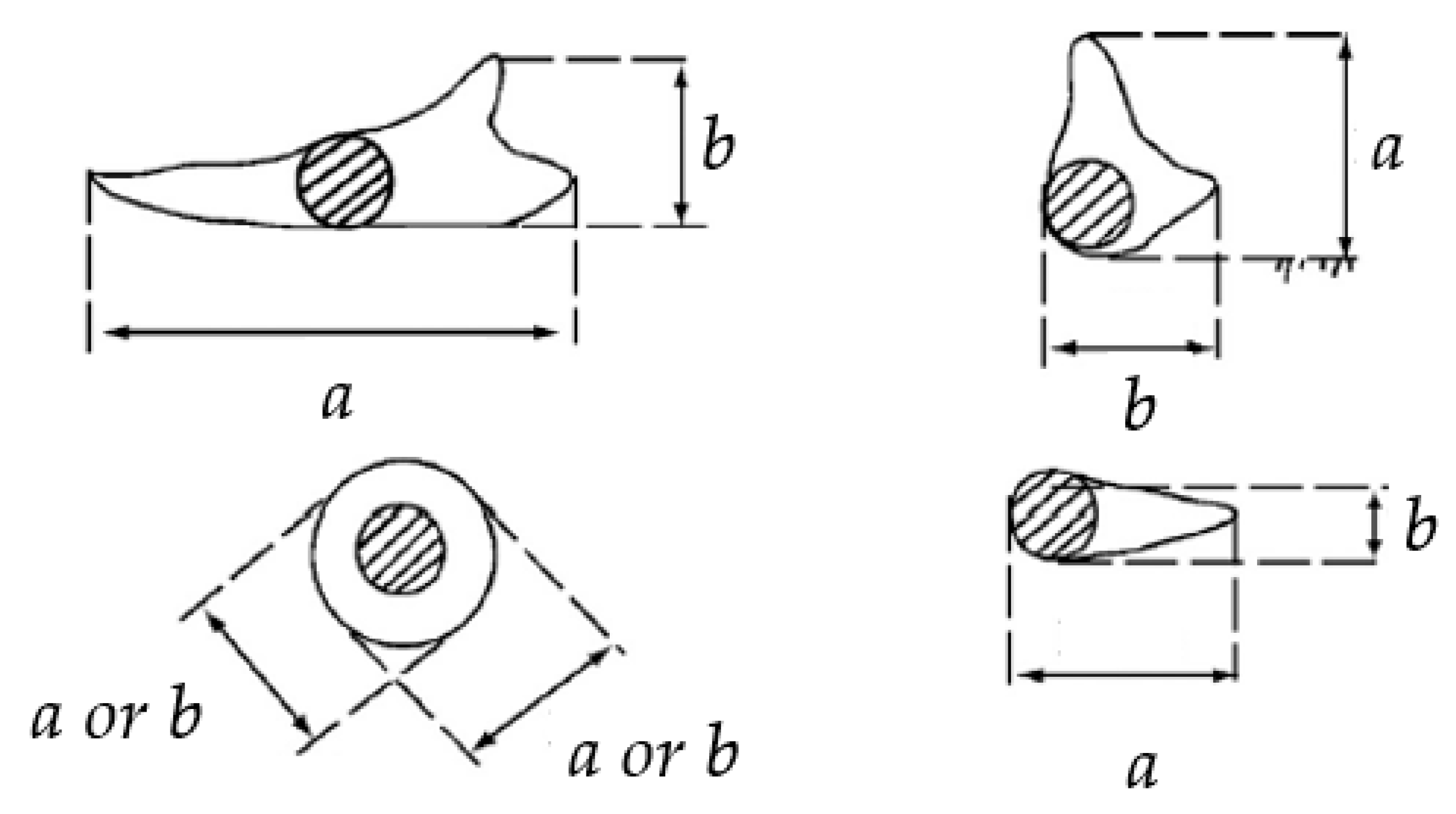
Table 1. A hotplate total precipitation sensor and a weather identifier and visibility sensor were set in the observation field of the Lushan Mountain Meteorological Bureau, approximately 2 m above the ground, continuously detecting the precipitation and visibility. The fog droplet spectrometer was approximately 1 m above the ground in the observation field, and was switched on during fog occurrence. In the winter of 2015/2016, wires were placed along the east–west, north–south and northeast–southwest directions on a 10 m tower on the west side of the observation field. During the winter of 2016/2017, wires were placed along the east–west and north–south directions at an empty location outside the observation field, and the ice frame was approximately 3.5 m above the ground. The wire diameters were all 26.8 mm, and the ice diameter
a (the maximum accumulated ice on the cut surface perpendicular to the wire, including the wire diameter, units: mm) and ice thickness
b (the maximum accumulated ice perpendicular to the ice diameter on the cut surface of the wire, units: mm) were measured hourly [
34] by a vernier caliper (
Figure 2). Wind, temperature, and humidity probes (see
Table 1) were installed at the same height as the ice frame.
Four longer-duration wire icing cases were acquired from the two years of observations, and data on the ice thickness, weather phenomena, meteorological elements, and fog spectrum were collected with a higher temporal resolution and greater reliability. Limited by the observations and severe weather conditions, the ice thickness data of the northeast–southwest wire were selected for cases 1 and 2 (the winter of 2015/2016), which represented the average icing conditions of the wires (along east–west and north–south directions). In cases 3 and 4 (the winter of 2016/2017), a mainly northerly wind was observed; therefore, the east–west wire was selected for study. The wire diameter is
(mm), the equivalent ice diameter is
D (mm), and the equivalent ice thickness is
W (mm), with calculation formulas as follows:
The ice thickness (mentioned later) was the equivalent ice thickness. During the icing periods, the frozen blade-type anemometer resulted in a zero wind speed; thus, the ice on it was removed from time to time, and such (zero) data were removed during the data processing. Nonzero wind data might have been collected when the ice was not completely removed, which means that the wind speed could have been underestimated; however, this is inevitable for freezing weather, and the wind speed data still have a reference value.
3. Overview of Four Icing Cases
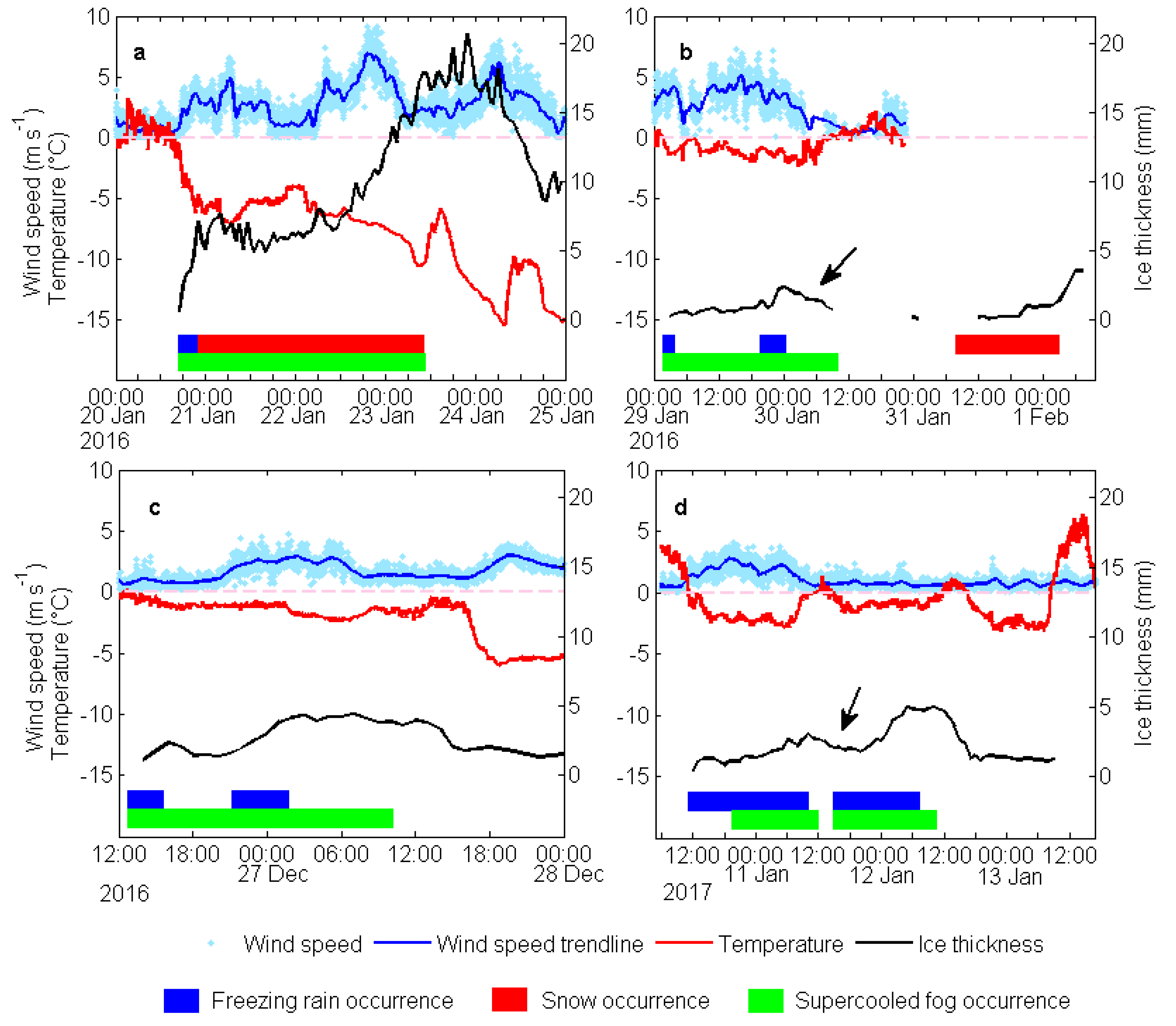
Figure 3 and
Table 2 show the ice thickness, temperature, wind speed, precipitation rate (rain and snow were both measured using the hotplate total precipitation sensor and are collectively referred to as the precipitation rate), fog liquid water content (FLWC), fog droplet number concentration (
NF), fog droplet mean diameter (
DF), and freezing rain, snow, and supercooled fog durations (LST, LST = UTC + 8 h, hereinafter inclusive) during the four icing cases. The freezing rain, snow, and supercooled fog occurrences were evaluated by the combination of manual observation records and weather phenomenon codes from the weather identifier and visibility sensor. In addition, all three types of weather occurrence evaluations required air temperatures of less than 0 °C at the same height as the wire, and the supercooled fog occurrence evaluations required visibility values below 1 km.
All four icing cases began with freezing rain, and the initial icing temperature was from −1.8 to −0.8 °C (
Figure 3 and
Table 2). The icing duration (102 h) and ice thickness (maximum 20.7 mm) of case 1 were much greater than those of the other three cases. There were three reasons for this. First, the rain (14 h) and snow (60 h) in case 1 lasted for the longest time. Second, in case 1, the temperature during icing remained below 0 °C, the temperature drop rate (−0.2 °C h
−1) was the highest, and the average temperature (−8.2 °C) was the lowest among the four icing cases, and these conditions were beneficial to the freezing of raindrops, fog droplets, and snow particles on the wire surface [
33]. The temperature during case 3 also remained below 0 °C, but the lowest temperature (−6.0 °C, 18:43 on 27 Dec 2016) was higher than that of case 1 (−15.5 °C, 07:56 on 24 Jan 2016). The temperatures in cases 2 and 4 exceeded 0 °C (10:05–21:42 on 30 Jan 2016, 11:05–15:05 on 11 Jan 2017, 11:43–16:24 on 12 Jan 2017) and reached a maximum of 2.1 °C (16:59 on 30 Jan 2016), during which the ice melted. Finally, the case 1 wind speed (3.1 m s
−1) was the highest among the four icing cases. The wind was beneficial for heat dissipation at the ice surface and led to increases in the horizontal particle flow [
9] and collision efficiency (the ratio of the flux density of the particles that hit the object to the maximum flux density) between the particles and wires [
24,
27,
31].
The characteristics of the four cases of icing were different. Cases 1 and 2 had lower temperatures, and their weather type was mainly snow and supercooled fog with a lower liquid water content, and these snow particles and fog droplets froze quickly after adhering to the wire. A dry growth was observed, and the ice was white with a lower density. The temperatures of cases 3 and 4 were relatively high, and their weather type was mainly freezing rain with a higher liquid water content, which converged and flowed along the wire surface after adhering to it. A wet growth was observed, and the ice was uniform and transparent and had almost no bubbles.
4. Distributions of Icing Growth Rates in Freezing Rain, Snow, and Supercooled Fog
To reduce the influence of measurement errors and other factors, a five point moving average of the ice thickness data of cases 1–4 during the icing growth period was determined. The hourly icing growth rate of the four icing cases was then calculated, and a total of 101 icing growth rate samples were obtained and classified for freezing rain, snow, and supercooled fog. The three types of weather occurrence evaluations were consistent with those in
Section 3. The freezing rain and snow appeared mixed with supercooled fog for most of the durations of the four icing cases; therefore, the freezing rain and snow mentioned below were actually freezing rain mixed with supercooled fog and snow mixed with supercooled fog, while the supercooled fog mentioned below was pure fog (no simultaneous rain or snow). The distributions of the icing growth rates in the three types of weather and their influencing factors were analyzed.
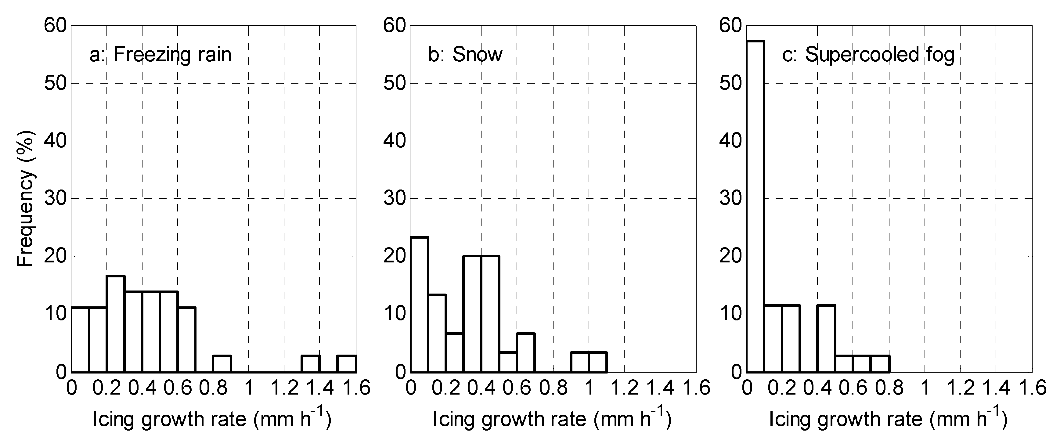
Figure 4 shows the icing growth rate frequency distributions in freezing rain, snow, and supercooled fog. The average icing growth rates of freezing rain, snow, and supercooled fog were 0.4, 0.3, and 0.2 mm h
−1; the standard deviations were 0.3, 0.3, and 0.2; the highest frequencies appeared at 0.2–0.3, 0.0–0.1, and 0.0–0.1 mm h
−1; the ratios above 0.5 mm h
−1 were 33.3%, 16.7%, and 8.6%; and the maximum values were 1.6, 1.1, and 0.7 mm h
−1, respectively. The ice accumulation was the fastest in freezing rain for the following reasons. First, the average precipitation rate of the freezing rain was 0.8 mm h
−1, which indicated sufficient rainfall. Second, the sticking efficiency
β (ratio of the flux density of the particles that stick to the object to the flux density of the particles that hit the object) of the wires to the raindrops was close to 1, which was higher than the
β value of the wires to snow, which was dependent on the liquid water content of the snow [
21,
24]. Finally, the typical raindrop radius is 100-fold greater than that of a fog droplet [
36]; therefore, raindrops can provide abundant supercooled water for ice accumulation; moreover, because of their larger volume, the inertial force of raindrops is greater than that of fog droplets, which hinders raindrops from flowing around the wire and leads to a higher collision efficiency [
24,
27]. Because the FLWC in case 1 and the wind speeds in cases 3 and 4 were lower, the icing growth rate in supercooled fog was lower than that of the previous rime observations [
17,
27]. For example, the icing growth rate in supercooled fog calculated by Zhou et al. [
17] was 0.4 mm h
−1, which is twice as high as that in our study.
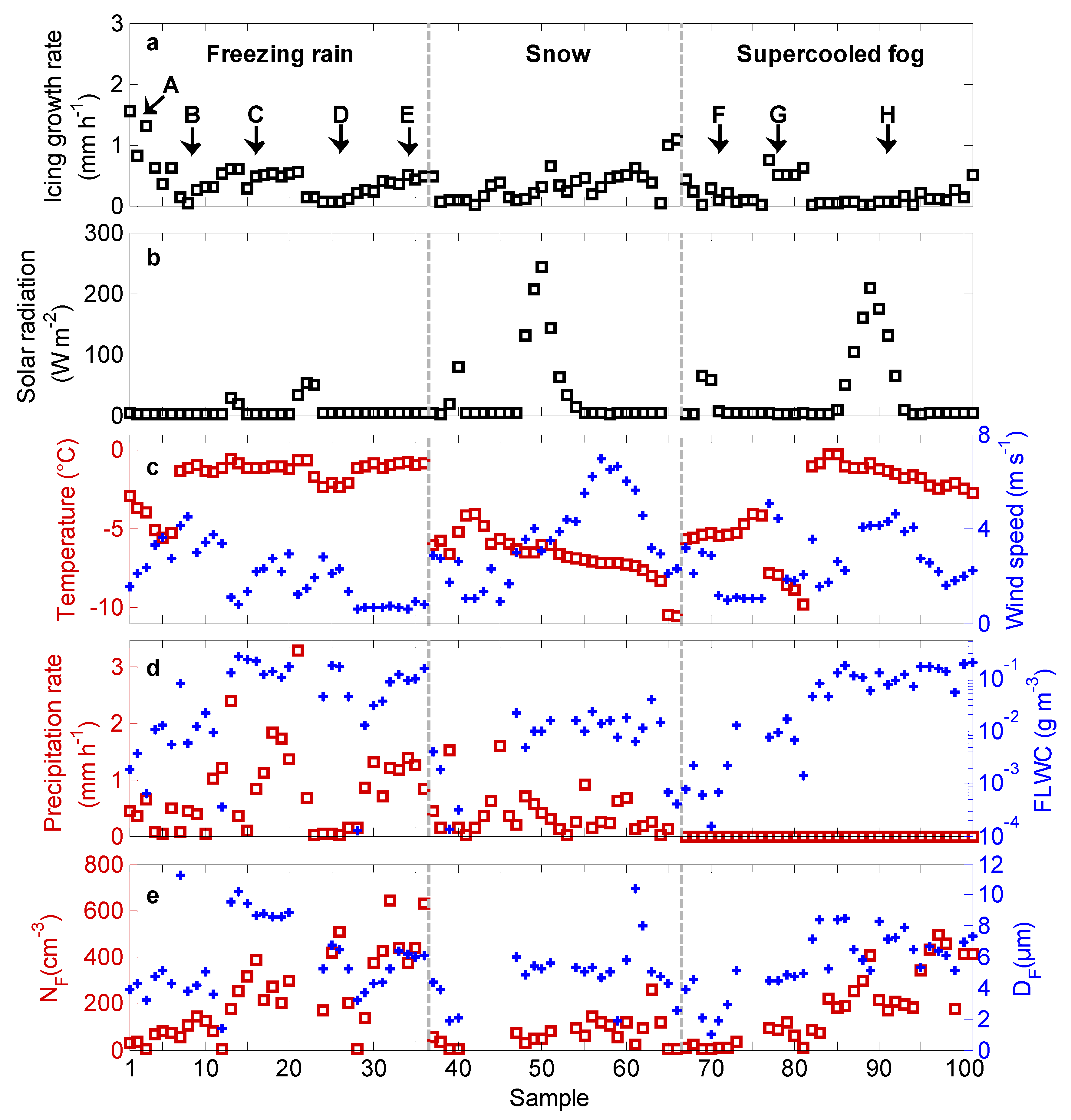
Figure 5a shows the distributions of the icing growth rate samples from the four icing cases for the three types of weather. The icing growth rate in each weather was arranged in chronological order, respectively.
Figure 5b–e shows the corresponding hourly average meteorological elements, precipitation rate, and fog droplet microphysical parameters. The average temperatures of the freezing rain, snow, and supercooled fog were −1.7, −6.7, and −3.5 °C, respectively, and supercooled fog had the largest temperature span (from −9.8 to −0.2 °C). The average wind speeds of the freezing rain, snow, and supercooled fog were 2.0, 3.6, and 2.6 m s
−1, respectively; the freezing rain and supercooled fog had lower wind speeds due to stable stratification.
The weather type of samples 1–36 was freezing rain. The temperature was lower for samples 1–3 (−3.5 °C), the precipitation rate increased significantly for samples 12–21 and 29–36 (means of 1.4 and 1.1 mm h
−1, respectively), and the ice grew rapidly during these three periods, with average growth rates of 1.2, 0.5, and 0.4 mm h
−1, respectively (arrows A, C, and E in
Figure 5). The freezing rain was weaker for samples 7–8 and 24–28 (average precipitation rates of 0.3 and 0.1 mm h
−1, respectively), and the average icing growth rate dropped to 0.1 mm h
−1 during both periods (arrows B and D in
Figure 5).
The weather type of samples 37–66 was snow. The icing growth rate and temperature during the snow showed opposite change trends, i.e., the icing accelerated with the decreasing temperature. Snow appeared along with supercooled fog in our study, and wires covered with rime or hoarfrost or a surface wetted by simultaneously impinging water droplets were conducive to capturing snow particles [
20]. Cooling promoted the rapid freezing of snow particles mixed with fog droplets.
The weather type of samples 67–101 was supercooled fog. For samples 77–81, the temperature was lower (−8.6 °C), and the wind speed was higher (maximum 5.1 m s
−1). The FLWC,
NF, and
DF were 0.008 g m
−3, 73 cm
−3, and 4.7 μm, respectively. The ice thickness increased significantly (0.6 mm h
−1, arrow G in
Figure 5). For samples 67–76, the FLWC,
NF, and
DF were lower (0.003 g m
−3, 14 cm
−3, and 3.1 μm, respectively), the temperature and wind speed were –5.1 °C and 1.7 m s
−1, respectively, and the icing growth was slower (0.2 mm h
−1, arrow F in
Figure 5). For samples 82–101, the FLWC,
NF, and
DF increased to 0.115 g m
−3, 270 cm
−3, and 6.8 μm, respectively, but the temperature rose to −1.5 °C and the wind speed dropped to 2.9 m s
−1, resulting in a slow icing growth rate (0.1 mm h
−1, arrow H in
Figure 5).
5. Correlations between the Icing Growth Rates and Meteorological Elements and Ice Thickness in Freezing Rain, Snow and Supercooled Fog
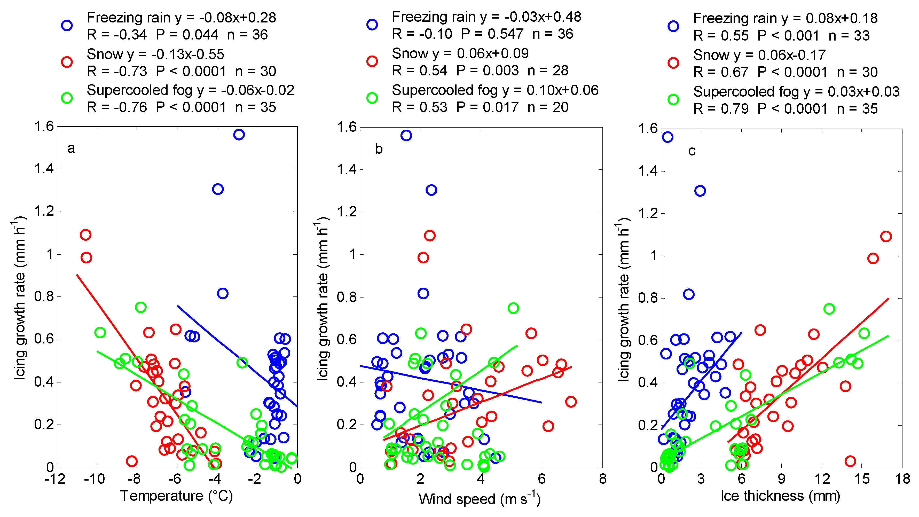
Figure 6a shows the correlation between the hourly mean temperature and the hourly icing growth rate in the three types of weather. In the snow and supercooled fog, the correlation coefficients between the temperature and the icing growth rate were −0.73 and −0.76, respectively, passing the significance test at the 0.0001 level. The slope of the fitted line was higher in snow (−0.13) than in fog (−0.06) because the snow particle volume was larger than the fog droplet volume; thus, the snow more easily collided with and froze on the wire, and the icing growth rate in snow increased faster than that in fog as the temperature decreased. The correlation between the temperature and icing growth rate under freezing rain was poor, because the temperature range for freezing rain is relatively narrow.
Figure 6b shows the correlation between the hourly mean wind speed and the hourly icing growth rate in the three types of weather. The icing growth rates in snow and supercooled fog presented increasing trends as the wind speed increased (
Figure 6b fitted lines), although the goodness of fit of all samples was lower. The goodness of fit was improved after eliminating the maximum and minimum icing growth rates, which were greatly affected by the temperature. In snow, the correlation coefficient between the wind speed and icing growth rate in the range of 0.00–0.80 mm h
−1 was 0.54, passing the significance test at the 0.01 level; in supercooled fog, the correlation coefficient between the wind speed and icing growth rate in the range of 0.07–0.80 mm h
−1 was 0.53, passing the significance test at the 0.02 level. Comparing the three types of weather, it was revealed that the slope of the fitted line was higher in supercooled fog (0.10) than in snow (0.06), and no obvious positive relationship between the wind speed and icing growth rate was observed in freezing rain. The flow of particles colliding with the wire is the vector sum of the vertical and horizontal mass flows [
9]. The fog droplet volume was the smallest among the three types of water sources; thus, the fog droplets were the most susceptible to the effects of the horizontal wind on the original trajectory and the resulting increase in the horizontal particle flow. Therefore, the increase in the icing growth rate as the horizontal wind speed increased was most obvious in the supercooled fog, and the slope of the fitted line was the largest. Due to the larger inertia force, the original trajectory of the raindrop was not easily affected by the horizontal wind; the icing growth rate was greatly affected by the vertical particle flow, and its relationship with the wind speed was not obvious.
Figure 6c shows the correlation between the hourly ice thickness and the hourly icing growth rate in the three types of weather. In freezing rain, the correlation coefficient between the ice thickness and icing growth rate in the range of 0.00–0.80 mm h
−1 was 0.55, passing the significance test at the 0.001 level. In snow and supercooled fog, the icing growth rates were both positively correlated with the ice thickness, with correlation coefficients of 0.67 and 0.79, respectively, passing the significance test at the 0.0001 level. As the ice thickness increased, the surface of the iced wire increased to allow more precipitation particles and fog droplets to stick, and the icing accelerated. The slope of the fitted line was higher in freezing rain (0.08) than in snow (0.06) or supercooled fog (0.03), but the correlation was poorer. This was because the ice thickness (2.2 mm on average) and its range (0.2–5.2 mm) were both relatively small during the freezing rain in our four icing cases; more icing cases need to be collected to analyze the relationship between the ice thickness and icing growth rate.
In conclusion, the correlations between the temperature and wind speed and the icing growth rate were stronger in snow and supercooled fog than in freezing rain. With the decrease in the temperature, the icing growth rate in the snow increased faster, while that in the supercooled fog increased faster as the wind speed increased. In freezing rain, snow, and supercooled fog, the icing growth rates were all positively correlated with the ice thickness, with correlation coefficients of 0.55, 0.67 and 0.79, respectively.
6. Impermanent Ice Shedding Phenomenon in Freezing Rain and Supercooled Fog
Ice shedding includes three mechanisms; melting, sublimation, and mechanical breaking [
13], and it usually occurs at the end of the icing period under changed weather conditions. The phenomenon in which ice was shed temporarily during a growth period and then grew again was observed in cases 2 and 4 (arrows in
Figure 3b,d). The shedding durations were both more than 9 h, and the ice thickness decreased by more than 40%. The observations and simulations should focus on the "inflection points" of the ice accumulation.
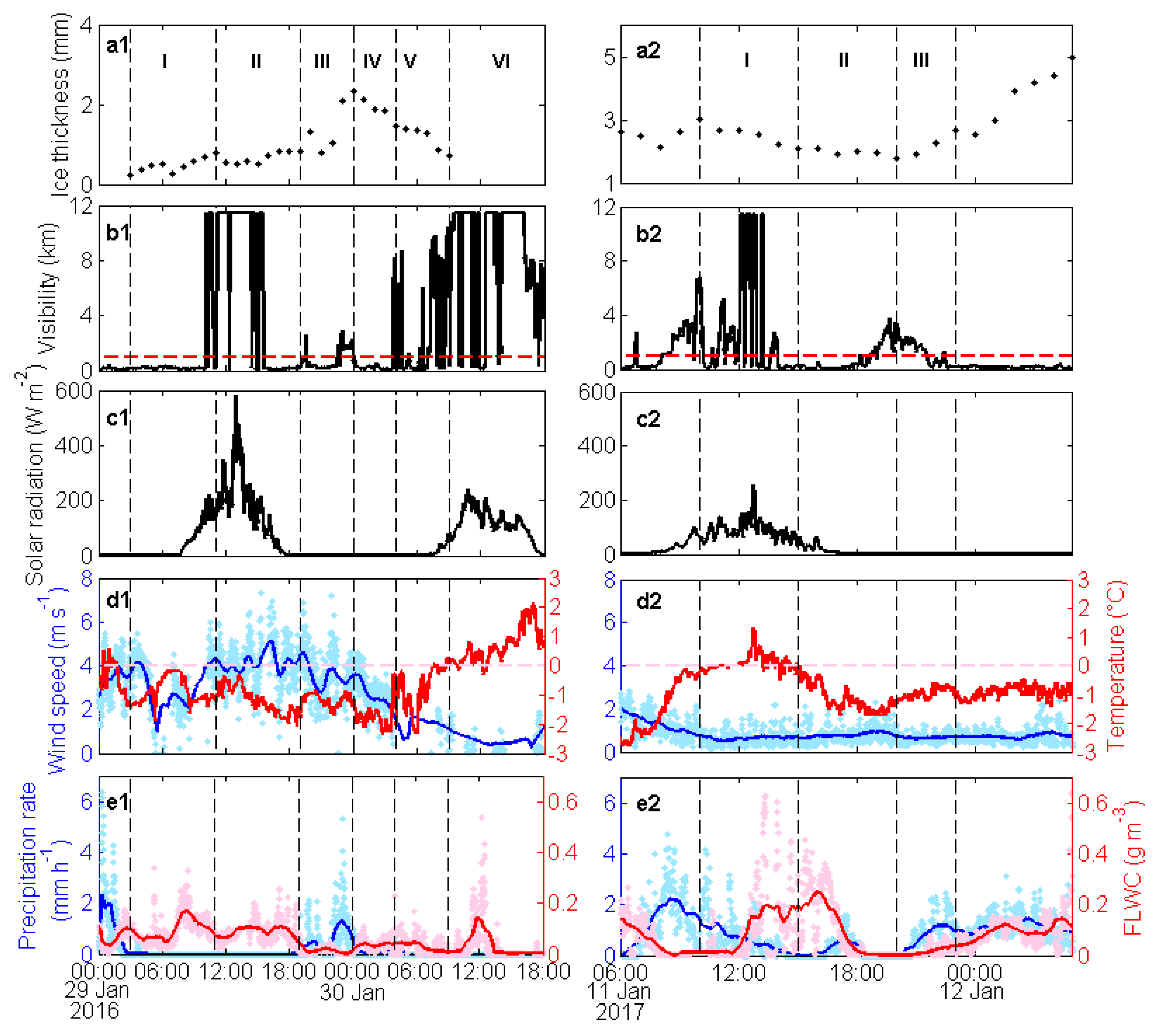
Figure 7 shows the temporal variations in the ice thickness, meteorological elements, precipitation rate, and FLWC during the impermanent ice shedding periods of cases 2 and 4. According to the variations in the ice thickness, they were divided into phases I–VI (
Figure 7(a1)) and phases I–III (
Figure 7(a2)).
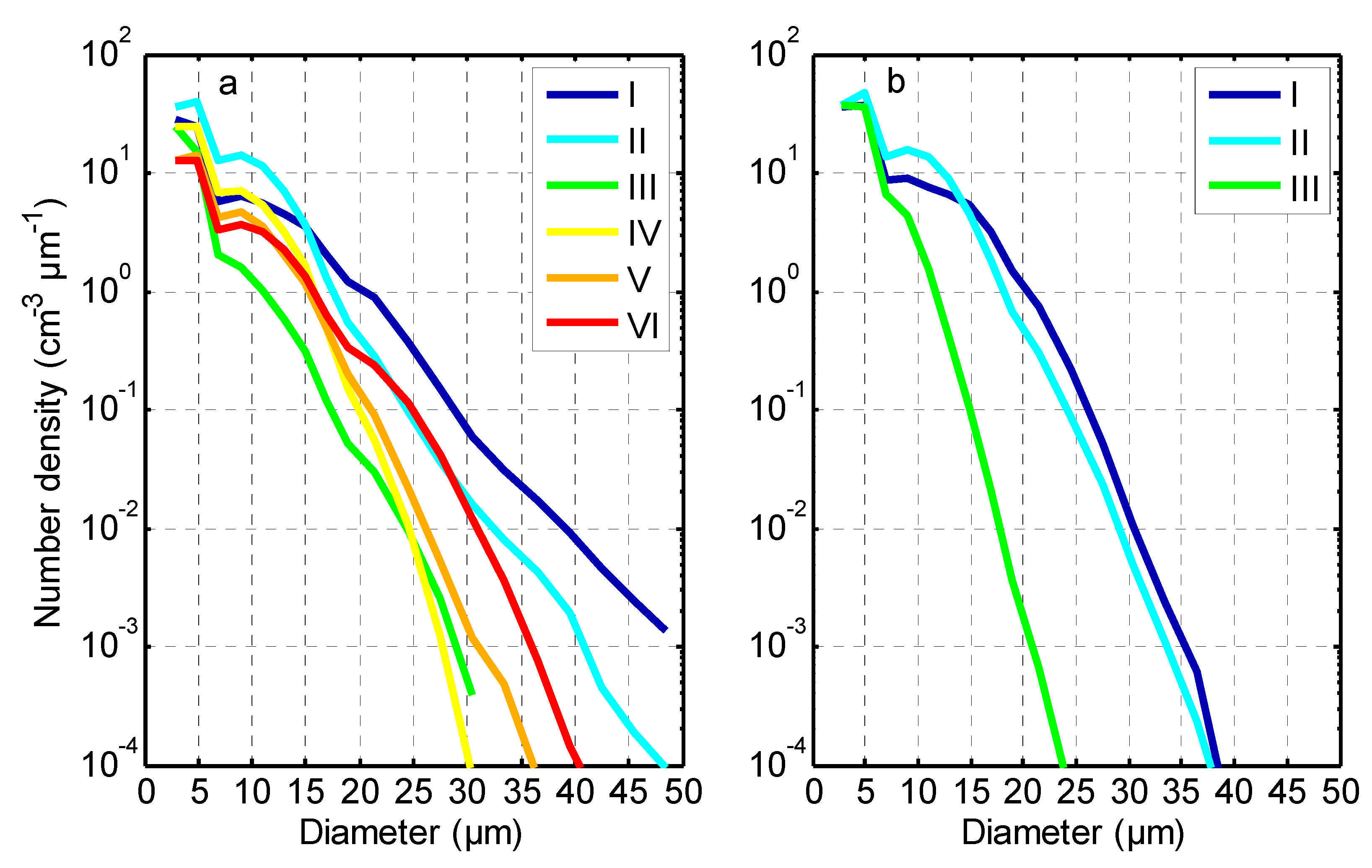
Table 3 and
Figure 8 show the ice shedding rate, meteorological elements, and fog droplet spectrum of each phase of
Figure 7. The causes of the impermanent ice shedding phenomenon were analyzed as follows.
In case 2-I, the fog droplet number density for the 15–50 μm particles (
Figure 8) and FLWC (0.095 g m
−3) (
Table 3) were the highest in each phase, and the ice thickness increased from 0.2 to 0.8 mm (
Figure 7). In case 2-II, the fog droplet number density for the 2–15 μm particles increased and that for the 15–50 μm particles decreased (
Figure 8), resulting in a slight decrease in the FLWC (0.087 g m
−3,
Table 3), although the wind speed (4.1 m s
−1,
Table 3) was the highest in each phase and the ice thickness remained stable (
Figure 7). In case 2-III, freezing rain appeared from 19:42 on 29 to 00:00 on 30 Jan 2016 (
Figure 7). The precipitation rate reached a peak of 5.3 mm h
−1 at 23:07 on 29 Jan 2016 (
Figure 7), and the average precipitation rate was the highest in each phase (0.6 mm h
−1,
Table 3). The icing growth rate (0.3 mm h
−1,
Table 3) was much larger than that of the first two freezing-rain-free phases, and the ice thickness reached a peak of 2.3 mm at 00:00 on 30 Jan 2016 (
Figure 7). In case 2-IV, the freezing rain intensity decreased (0.1 mm h
−1,
Table 3) and completely stopped at 00:25 on 30 Jan 2016 (
Figure 7); therefore, the weather type was mainly supercooled fog (visibility 0.4 km,
Table 3). In cases 2-I and II, the weather types of which were also mainly supercooled fog, the ice thickness slightly increased or remained stable (
Figure 7), while in case 2-IV, ice shedding occurred from 00:00 on 30 Jan 2016 (−0.2 mm h
−1,
Figure 7 and
Table 3). The wind speed (2.7 m s
−1,
Table 3), fog droplet number density in every spectral range (
Figure 8), and FLWC (0.036 g m
−3,
Table 3) in case 2-IV were all lower than those in cases 2-I and II. Moreover, the ice thickness was low and the structure was loose, facilitating sublimation and mechanical breaking; thus, the amount of ice accumulated was exceeded by the amount of ice lost to breaking and sublimation. In case 2-V, the temperature increased (−0.8 °C,
Table 3) and the wind speed decreased (1.2 m s
−1,
Table 3). The fog droplet number density for the 2–17 μm and 17–50 μm particles decreased and increased slightly (
Figure 8), respectively, the FLWC declined (0.027 g m
−3,
Table 3), and the icing continued to fall off (−0.1 mm h
−1,
Table 3). In case 2-VI, the temperature gradually rose with the enhanced solar radiation after sunrise (the highest value was 243.0 W m
−2 at 10:46 on 30 Jan 2016,
Figure 7), and it fluctuated around 0 °C from 07:32 to 10:00 on 30 Jan 2016 and exceeded 0 °C at 10:05, and the ice was shed completely at 10:00 (
Figure 7). The temperature dropped below 0 °C at 21:42 on 30 Jan 2016, and at 12:00 on 31 Jan 2016, ice began to grow again with the snowfall.
In case 4-I, the rain was stronger (0.7 mm h
−1,
Table 3), but the solar radiation reached a peak of 258.0 W m
−2 (12:44 on 11 Jan 2017,
Figure 7). The temperature exceeded 0 °C at 11:05 on 11 Jan 2017, and it reached a maximum of 1.3 °C at 12:44 on 11 Jan 2017 (
Figure 7). The ice thickness decreased significantly due to melting (−0.2 mm h
−1,
Table 3). In case 4-II, the temperature dropped below 0 °C again (15:05 on 11 Jan 2017,
Figure 7), the rain intensity weakened (0.2 mm h
−1,
Table 3), and the fog droplet spectrum (
Figure 8) and FLWC (
Table 3) remained stable. The ice was not frozen completely, and its growth was not obvious (
Figure 7). In case 4-III, the temperature was below 0 °C, and the freezing rain strengthened (0.8 mm h
−1,
Table 3). Inhibited by the rainfall, the fog droplet number density in every spectral range (
Figure 8) and the FLWC (0.015 g m
−3,
Table 3) decreased. The fully frozen ice began to grow again under the influence of the freezing rain at 20:00 on 11 Jan 2017 (
Figure 7).
Ice was shed temporarily in supercooled fog when the temperature remained below 0 °C, the wind speed fell to 2.7 m s−1, and the fog liquid water content fell to 0.036 g m−3 (case 2, mechanical breaking and sublimation). In addition, ice was shed temporarily in freezing rain when the solar radiation increased and the temperature exceeded 0 °C (case 4, melting).
7. Icing Simulation
Icing models have been built previously for different ice-producing conditions, such as freezing rain, snow, and supercooled fog. In our four observed cases, mixed conditions were present, so suitable models and parameters to use for our cases were further explored.
7.1. Brief Introduction of the Models
7.1.1. Freezing Rain Ice Accumulation Model
Jones [
18] described freezing rain ice loads on a horizontal cylinder using a simple model according to the precipitation rate and wind speed. The ice thickness (
W, units: mm) was determined as follows:
where
P,
L, and
U are the precipitation rate (mm h
−1), liquid water content (g m
−3) of freezing rain, and wind speed (m s
−1) in the
jth minute of the freezing rain, respectively;
g cm
−3 represents the density of water, and
g cm
−3 represents the density of ice.
7.1.2. Wet Snow Ice Accumulation Model
Makkonen [
20] derived the wet snow ice accumulation model:
where
M represents the accumulated snow mass (g) per unit length,
D represents the equivalent ice diameter (m), and
I represents the accretion intensity per unit area (g m
−2 s
−1), which can be calculated by the following formula:
where
c represents the mass concentration of wet snow (g m
−3) in the air, which is usually calculated by the visibility
Vm (m):
In addition,
υs represents the terminal velocity of the snowflakes (approximately 1 m s
−1, on average [
20,
37]), and
β represents the sticking efficiency, which is usually calculated by the wind speed
U (m s
−1):
The ice diameter
D (m) was determined as follows:
7.1.3. Supercooled Fog Ice Accumulation Model
Makkonen [
24] summarized the ice accumulation models as follows:
where
M,
A,
ω, and
υ represent the ice weight (g), cross-sectional area of the object (m
2), liquid water content (g m
−3), and particle velocity (m s
−1), respectively, and
α1,
α2, and
α3 represent the collision efficiency, sticking efficiency, and accretion efficiency, respectively. The model can simulate different types of ice accumulations. Niu et al. [
16] used the model to simulate supercooled fog ice accumulation. In this study, this model was also used to calculate ice accumulation under supercooled fog conditions; therefore, the
ω is actually FLWC.
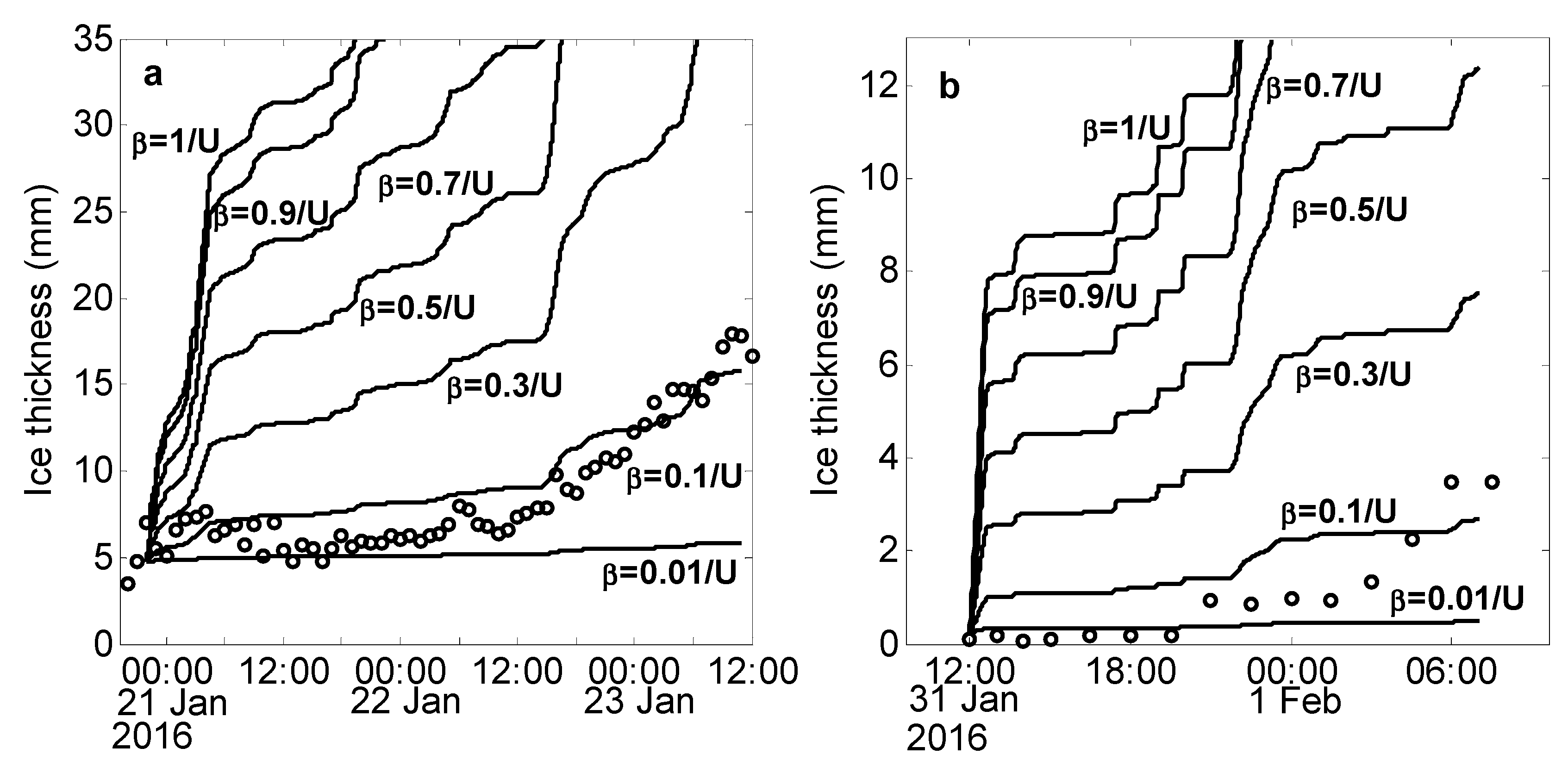
7.2. Model Localization Test
The sticking efficiency
β of the wire to snow particles requires further study [
20,
24], and a localization test was performed. Makkonen [
20] used a wet-bulb temperature
Tw higher than 0 °C to indicate wet snow occurrence and simulated its growth (with
). The snow in cases 1 and 2 had a lower temperature
T (
Figure 3 and
Table 2) (
°C), and dry snow occurred. As pointed out in previous studies [
24], dry snow particles rebound easily when colliding with wires, for which the
β is almost 0. However, supercooled fog appeared along with snow in cases 1 and 2, and dry snow particles could be partly captured by wires covered with rime or hoarfrost or by a surface wetted by simultaneously impinging water droplets [
20], for which the
β remains to be determined. As shown in
Figure 9, simulations performed using the Makkonen [
20] wet snow model directly (
) resulted in icing growth that was much faster than that of actual observations.
,
,
,
,
,
, and
were applied separately. When
, the simulation results better reflected the changes in the actual ice thickness. In the model of Makkonen [
20], when the wind speed
m s
−1, the
β value in the wet snow took the maximum value of 1.00; through the above localization test, the dry snow
β (
) in our study was 1/10 that of wet snow (
), so the maximum
β value was 0.10 during the dry snow in our observed cases. The maximum and average wind speeds in our two snow periods were 9.1 m s
−1 (19:13 on 22 Jan 2016) and 3.1 m s
−1, respectively, which corresponded to minimum and average
β values (
) of 0.01 and 0.03, respectively, and the variation range of
β for our observed cases was 0.01–0.10. Based on the weight and thickness of the snow deposits over our two years of observations,
ρi adopted a snow deposit average density of 0.2 g cm
−3 in the simulations, which is less than the wet snow deposit average densities used by Makkonen [
20] and Makkonen and Wichura [
12] of 0.4 and 0.3 g cm
−3, respectively. The wet snow accumulation is closer to the wet growth [
24], which has a higher density.
Zhou et al. [
17] and Niu et al. [
16] used the freezing rain icing model of Jones [
18] and the model of Makkonen [
24] to calculate the ice growth in freezing drizzle and supercooled fog at Enshi Radar Station in Hubei Province of China, and their results indicated that these two models have good applicability for precipitation and in-cloud icing simulations of high-altitude mountainous areas in China.
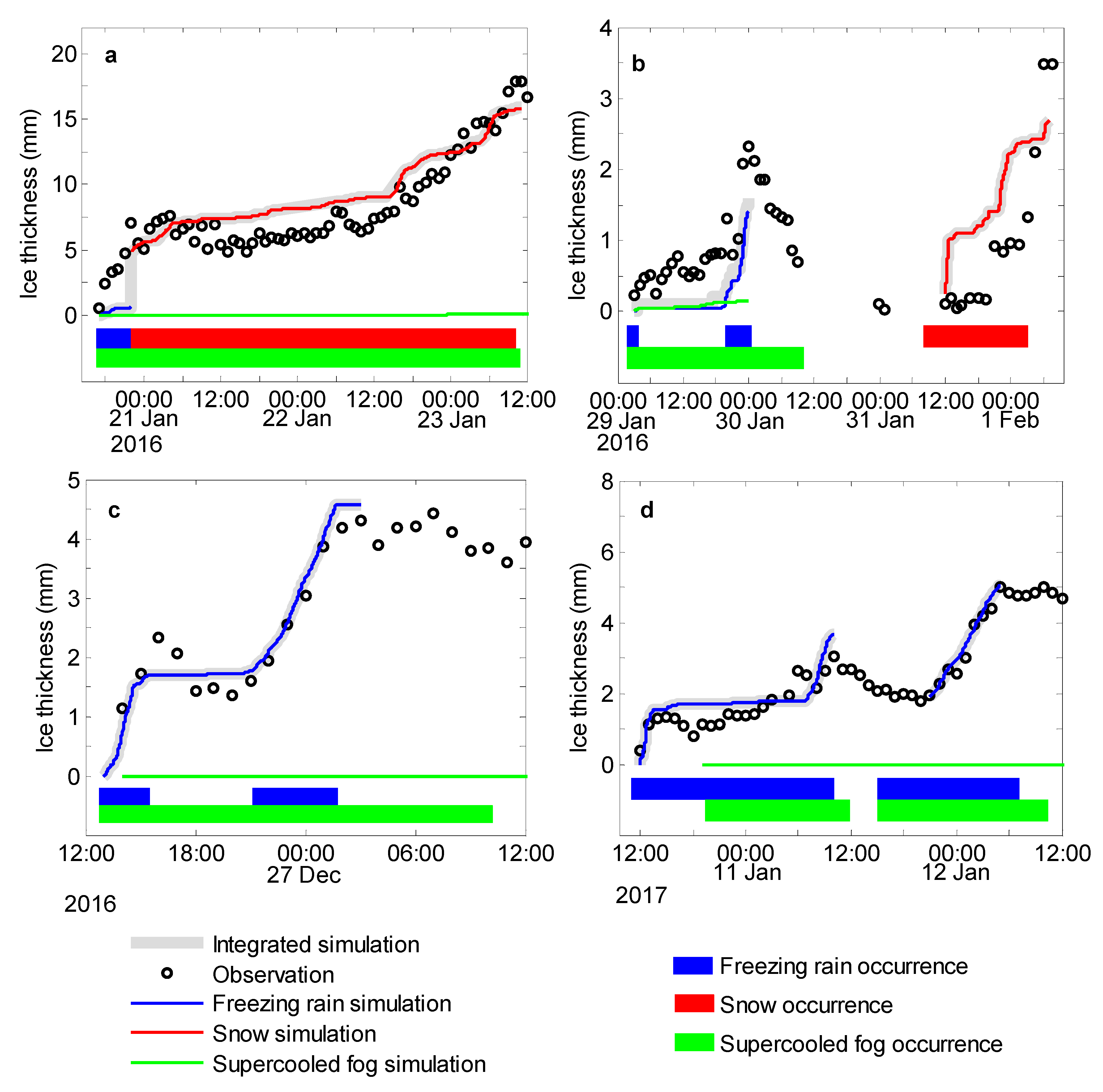
7.3. Simulation Results from the Freezing Rain, Snow, and Supercooled Fog Ice Accumulation Models
Taking the precipitation rate and wind speed during the period of freezing rain as inputs, the ice growth impacted only by freezing rain was calculated using the freezing rain ice accumulation model of Jones [
18] (blue line in
Figure 10). Taking the visibility and other parameters as inputs, the ice growth impacted by snow (red line in
Figure 10) was calculated using the modified snow accumulation model (
Section 7.2). Taking the FLWC and
DF as inputs, the ice growth influenced only by supercooled fog was calculated using the supercooled fog ice accumulation model of Makkonen [
24] (green line in
Figure 10). Since the three models cannot simulate ice shedding, segmented simulations were carried out for the impermanent ice shedding periods of cases 2 and 4 (
Section 6).
The ice thickness growth simulated by the supercooled fog model was not obvious in cases 1, 3, and 4. Equation (9) in the model of Makkonen [
24] shows that a lower particle velocity (
υ) and liquid water content (
ω) cause the supercooled fog icing to grow slowly. Due to the discontinuity of the supercooled fog and the scouring of raindrops and snow particles on fog droplets [
38], the FLWC in case 1 (
Table 2) was lower than that of previous microphysical observations of in-cloud icing [
16,
39,
40], and the direct contribution of supercooled fog to the ice accumulation was relatively small. The FLWCs of cases 3 and 4 were higher than that of case 1, but their wind speeds were lower than that of the previous in-cloud icing observations [
27] (
Table 2). Due to the fog droplet’ smaller inertia force, the wind speed was the main factor affecting its particle velocity
υ, and the supercooled fog ice growth was slow. For example, from 16:00 to 20:00 on 26 Dec 2016 in case 3 and from 15:00 on 10 Jan to 06:00 on 11 Jan 2017 in case 4, no freezing rain or snow occurred, and only supercooled fog appeared (average fog liquid water content of 0.244 g m
−3) and the ice growth was slow (0.0 mm h
−1 on average). Compared with cases 1, 3, and 4, the supercooled fog had a relatively large contribution to the ice accumulation in case 2.
7.4. Integrated Model Simulation Results
Freezing rain, snow, and supercooled fog appeared in combination in the four icing cases. The simulation results of the three models were added together, and the resulting ice thickness can better reflect the changes in the actual ice thickness (gray line in
Figure 10). Thus, an integrated ice accumulation model was built: if freezing rain occurs, the freezing rain ice accumulation model starts; if snow occurs, the snow ice accumulation model starts; if supercooled fog occurs, the supercooled fog ice accumulation model starts; the simulated ice thicknesses of the three models are then added together.
Table 4 shows the relative error (
) and root mean square error (
RMSE) between the integrated model simulated values and the observed values of the four icing cases. The calculation formulas were as follows:
where
xobs,j,
xmodel,j, and
n represent an observed value, a simulated value, and the sample size, respectively. Cases 1, 3, and 4 showed better simulations, while case 2 had a higher relative error. This is because the observed ice thickness in case 2 was less than 2 mm most of the time, which led to the smaller denominator of Equation 10. As the wind speed measured by the blade-type anemometer in freezing weather might be less than the actual values (
Section 2), the ice thickness simulation values might be less than the actual values. This was relatively obvious from 03:00 on 29 Jan to 00:00 on 30 Jan 2016 in case 2 (
Figure 10b) because the supercooled fog made a relatively large contribution to the ice accumulation in this period (
Section 7.3); compared with the freezing rain and snow, the icing growth rate in the supercooled fog was more sensitive to wind speed (
Section 5). The ice was shed temporarily from 00:00 on 30 Jan to 11:00 on 31 Jan 2016 in case 2. From 12:00 to 18:00 on 31 Jan 2016, the ice accretion was slower in the initial period of refreezing. The ice growth model did not sufficiently account for this phenomenon, and the simulated values from 12:00 on 31 Jan to 03:00 on 1 Feb 2016 in case 2 were thus higher than the actual values (
Figure 10b). However, overall, the simulation results well reflected the actual ice thickness change trend in case 2.
8. Conclusions
Two years of observations at the Lushan Mountain Meteorological Bureau were assessed to obtain data on four wire icing cases. For cases 1, 2, 3, and 4, the initial icing temperatures were −1.8, −1.4, −0.8, and −0.8 °C; the maximum ice thicknesses were 20.7, 3.5, 4.4, and 5.0 mm; and the icing durations were 102, 77, 34, and 69 h, respectively. The ice in cases 1 and 2 was white with a lower density, and the ice in cases 3 and 4 was transparent with a higher density.
The average icing growth rates in freezing rain, snow, and supercooled fog were 0.4, 0.3, and 0.2 mm h−1; the standard deviations were 0.3, 0.3, and 0.2; the highest frequencies appeared at 0.2–0.3, 0.0–0.1, and 0.0–0.1 mm h−1; the ratios above 0.5 mm h−1 were 33.3%, 16.7%, and 8.6%; and the maximum values were 1.6, 1.1, and 0.7 mm h−1, respectively.
The correlations between the temperature and wind speed and the icing growth rate were stronger in snow and supercooled fog than in freezing rain, and the correlation coefficients between the temperature and the icing growth rate in snow and supercooled fog were −0.73 and −0.76, respectively. With the decrease in the temperature, the icing growth rate in the snow increased faster, and the icing growth rate in the supercooled fog increased faster as the wind speed increased. In freezing rain, snow, and supercooled fog, the icing growth rates were all positively correlated with the ice thickness, with correlation coefficients of 0.55, 0.67, and 0.79, respectively.
Temporary ice shedding occurred in supercooled fog (mechanical breaking and sublimation) when the temperature remained below 0 °C, the wind speed fell to 2.7 m s−1, and the FLWC fell to 0.036 g m−3, and it occurred in freezing rain (melting) when the solar radiation increased and the temperature exceeded 0 °C.
Based on the observation data of our four icing cases, a localization test for the sticking efficiency in the snow accumulation model was performed. When the sticking efficiency of the wire to the snow particles was 0.1/U, the snow accumulation model could better simulate the ice thickness in snow in Lushan. Calculated from the wind speed (U), the average sticking efficiency during snowfall was 0.03, and its variation range was 0.01–0.10. Icing models have been built in previous studies for different ice-producing conditions, such as freezing rain, snow, and supercooled fog. In our observed four cases though, mixed conditions were present. A model was established by integrating the three ice accumulation models of freezing rain, snow, and supercooled fog: if freezing rain occurs, the freezing rain ice accumulation model is employed; if snow occurs, the snow ice accumulation model is employed; and if supercooled fog occurs, the supercooled fog ice accumulation model is employed. The simulated ice thicknesses of the three models are then added together. The simulation results of the integrated model can better reflect the changes in the actual ice thickness.
The icing growth and shedding mechanisms in freezing rain, snow, and supercooled fog were classified and compared in our study to reveal different icing patterns. A model was established by integrating freezing rain, snow, and supercooled fog ice accumulation models, and the integrated model is suitable for mixed icing conditions. The types of precipitation still need more detailed classification, such as accounting for sleet. This transitional precipitation was short lived in our four icing cases, and more cases need to be collected. If there are more abundant data, such as the fall velocity of the precipitation particles, the precipitation type discrimination criteria should be established for the integrated icing model. The applicability of the integrated model still needs to be verified and improved at different sites. Moreover, the ice growth model cannot accurately simulate the phenomenon in which ice is shed temporarily and then continues to grow. Few ice shedding models are available, and simulation studies of ice shedding are still required. Icing simulation studies must be strengthened to improve frozen disaster prediction systems.


