A Combined Model Based on Feature Selection and WOA for PM_2.5 Concentration Forecasting

Abstract

As people pay more attention to the environment and health, $P{M}_{2.5}$ receives more and more consideration. Establishing a high-precision $P{M}_{2.5}$ concentration prediction model is of great significance for air pollutants monitoring and controlling. This paper proposed a hybrid model based on feature selection and whale optimization algorithm (WOA) for the prediction of $P{M}_{2.5}$ concentration. The proposed model included five modules: data preprocessing module, feature selection module, optimization module, forecasting module and evaluation module. Firstly, signal processing technology CEEMDAN-VMD (Complete Ensemble Empirical Mode Decomposition with Adaptive Noise and Variational Mode Decomposition) is used to decompose, reconstruct, identify and select the main features of $P{M}_{2.5}$ concentration series in data preprocessing module. Then, AutoCorrelation Function (ACF) is used to extract the variables which have relatively large correlation with predictor, so as to select input variables according to the order of correlation coefficients. Finally, Least Squares Support Vector Machine (LSSVM) is applied to predict the hourly $P{M}_{2.5}$ concentration, and the parameters of LSSVM are optimized by WOA. Two experiment studies reveal that the performance of the proposed model is better than benchmark models, such as single LSSVM model with default parameters optimization, single BP neural networks (BPNN), general regression neural network (GRNN) and some other combined models recently reported.

1. Introduction

In recent years, with the improvement of people’s living standards, the problem of air pollution is also increasing. This is especially serious in China [1,2]. In the north, industrial development has resulted in serious deterioration of air quality over the past several decades [3,4,5]. A recent report by the State Environmental Protection Administration stated that two out of every five cities in China failed to meet the residential area air quality standard, resulting in the exposure of their population to the risk of adverse health effects. As a major pollutant, $P{M}_{2.5}$ have caused widespread concern over the country. $P{M}_{2.5}$ refers to fine particles with particles not larger than 2.5 um, which is extremely harmful to public health. There are two main sources of $P{M}_{2.5}$ in the air. On the one hand, it is mainly from the burning of fossil fuels, such as smelting, metal processing and transportation [6,7]. On the other hand, it comes from the chemical reaction of NO${}_2$, CO and SO${}_2$ in the atmosphere [8].

$P{M}_{2.5}$ can also adsorb a variety of toxic pollutants, including heavy metals, volatile organic compounds and carbonaceous materials. It has been reported that exposure to high concentrations of $P{M}_{2.5}$ leads to an increase in cardiovascular and pulmonary diseases (e.g., [9,10]). According to the American Heart Association, in the United States alone, air contaminated with $P{M}_{2.5}$ particles causes approximately 60,000 deaths per year. In addition, many epidemiological and panel studies have shown that a relationship exists between particulate matter (PM) in the air and the emergence of diseases such as short-term cardiopulmonary function [11], cerebrovascular disease [12], respiratory disease [13], lung cancer (e.g., [14]), etc. Further, particle size less than 0.1 microns, is referred to as “ultrafine particle” or “nanoparticles”. Experts from University of Nanjing Information Science and Technology have found that the concentration of ultra fine particles with a diameter of 0.01 to 0.1 um is significantly increased in Nanjing. Most of the particles floating in the air can stay in the lungs and enter the bloodstream, which is also an important reason for the recurrence of asthma and chronic bronchitis [13]. Therefore, the research and control of $P{M}_{2.5}$ is an urgent issue.

Many countries have established PM monitoring systems to monitor $P{M}_{2.5}$ concentrations in real time, which provide early warnings through analysis and prediction of data to help us adopting regulatory measures. However, due to the huge resource cost of establishing a testing site, or the completed site damaged by rain, human factors, etc., monitoring data may be incomplete or have drawbacks. Therefore, it is necessary to use methods and tools to analyze and model PM concentrations. Based on the above reasons, this paper attempts to propose a combined model to accurately predict $P{M}_{2.5}$ concentration.

In order to achieve high accuracy, previous literature has proposed many predictive tools and methods to predict $P{M}_{2.5}$ or other air pollutant concentrations [15,16]. These methods can be divided into two categories: the deterministic methods described by the chemical transport model (CTM) [17], and statistically based predictive methods. CTM is the most conventional method on $P{M}_{2.5}$ concentration prediction, which requires the acquisition of meteorological factors. The data acquisition of CTM is difficult and costly, and its prediction accuracy is not satisfying. Therefore, statistical methods [18] and machine learning [19] are widely used in the field of air pollutants prediction. The basic statistical methods are mainly originated from multiple linear regression (MLR) and autoregressive integrated moving average models (ARIMA) [20]. However, due to the complex nonlinear relationship between $P{M}_{2.5}$ and air quality [21], the two mentioned models cannot fit these nonlinearities, which causes the predicted value to be different with the actual value. With the rapid development of computer technology, a combined model using artificial intelligence method not only has the advantages of low cost and high prediction accuracy, but also has the nonlinear fitting characteristics, so can be well suited to the prediction of $P{M}_{2.5}$.

Artificial neural networks (ANN) (e.g., [22,23,24,25]), grey models (GM), generalized linear regression models, and support vector regression (SVR) [26,27] are widely used artificial intelligence models in the prediction of PM concentration. In addition, the parameters in these models, such as ANN and SVR [26,27], have a great influence on the prediction effect of the models [28]. Therefore, some swarm intelligent optimization algorithms, such as genetic algorithm (GA), particle swarm optimization algorithm (PSO) [29], gray wolf optimization algorithm (GWO), cuckoo optimization algorithm (CS) etc., have been used to optimize the parameters. After using these algorithms to optimize the model parameters, the models’ accuracy is increased and the robustness is improved. Paschalidou AK et al. [30] used the multilayer perceptron (MLP) with the radial basis function (RBF) techniques to forecast hourly $P{M}_{10}$ concentrations in four urban areas (Larnaca, Limassol, Nicosia and Paphos) of Cyprus. Feng X. et al. [31] proposed a hybrid model combining air mass trajectory analysis and wavelet transformation to improve ANN forecast accuracy of daily average concentrations of $P{M}_{2.5}$. Shi F. et al. [32] proposed a neural network model based on GWO, using the $P{M}_{2.5}$ data from 1 November to 22 November 2016, in Shanghai city. Furthermore, the results show that it is much better than neural network based on PSO, BPNN, and SVR. Yali F U et al. [33] proposed a hybrid model using the improved particle swarm optimization algorithm (IPSO) to optimize the number of hidden layer nodes and weights of the extreme learning machine (ELM). Wang L. et al. [34] proposed a $P{M}_{2.5}$ concentration rolling statistical prediction scheme (DC-SVR) based on distance correlation coefficient and SVR. Dai L. et al. [35] combined SVM and PSO algorithm to construct hourly $P{M}_{2.5}$ concentration rolling prediction model. Meanwhile, using the rolling model to predict the nighttime average concentration, daytime average concentration and daily average concentration of the next day. Gan K. et al. [36] proposed a new method based on the secondary-decomposition-ensemble learning paradigm. This model decomposed and reconstructed the raw data before prediction, and then predicted via the LSSVM model optimized by chaotic particle swarm optimization algorithm (CPSO) to obtain the predicted value. Data collected over seven years in a city of northern Spain are analyzed using four different models—vector autoregressive moving average (VARMA), ARIMA, MLP neural networks and SVM with regression, and simulations showed that the SVM model performs better than the other models when forecasting one month ahead and the following seven months [37]. Gualtieri G. et al. [38] forecasted $P{M}_{10}$ hourly concentrations in northern Italy through self-organizing maps. Zhou Q. et al. [39] proposed a hybrid ensemble empirical mode decomposition-general regression neural network (EEMD-GRNN) model based on data preprocessing to analysis for one-day-ahead prediction of $P{M}_{2.5}$ concentrations. Li W. et al. [40] used a hybrid model, cointegration theory-flower pollination algorithm-support vector machine (CI-FPA-SVM), to predict $P{M}_{2.5}$ and $P{M}_{10}$ concentration. Ping G et al. [41] proposed a framework, termed HML-AFNN, to analyse and forecast the concentration of particular matter ($P{M}_{2.5}$) for a selected number of forward time steps and so on [42]. From the above analysis, it is known that the prediction using the hybrid model is already a trend of PM concentration forecasting. However, in the prediction by hybrid model, the computational consumption is high because the input data are too large. If certain technology can significantly reduce the input data without affecting the prediction effect, this will be a big breakthrough.

Most researchers do not focus on optimizing the input-output features or doing a feature selecting work when they start to establish their model [43]. These models are unlikely to learn the essence of the time series, and thus there is a large gap between the predicted and the actual values. We hope to learn the model between the best input and the best output in the $P{M}_{2.5}$ series by adopting a completely automated machine learning method, so as to avoid artificially selecting the training relationship and establishing a more stable and accurate power load forecasting model.

ACF can find the dependence relationship between one time and other times in a time series. Hopefully this hidden input–output relationship can be automatically given by ACF feature selection techniques. LSSVM has strong learning ability for nonlinear relations. The WOA is used to optimize the parameters in LSSVM. Finally, the de-noised data are used to train the model. Therefore, we focus on using ACF and LSSVM, combined with WOA, to select good features for building a strong model. The established model can be used for the prediction of $P{M}_{2.5}$ concentration.

What is new about this paper is that the feature selection is added to the general hybrid model so that the computer can automatically select as few inputs as possible for any set of data without affecting the final prediction effect.

The rest of this paper is as follows: Section 2 describes the basic methods (CEEMDAN, VMD, ACF, WOA and LSSVM). Section 3 describes two data sets and experimental settings. Section 4 is comparative results; Section 5 is conclusions and further study.

2. Methods

The basic structure of the proposed model VCEEMDAN-SF-WOA-LSSVM is presented in Figure 1. First, signal processing technology CEEMDAN-VMD is used to decompose and reconstruct the $P{M}_{2.5}$ concentration series, then ACF is used to extract the input variables. Finally, LSSVM is applied to predict, and the parameters of LSSVM are optimized by WOA. The required methods that were applied in the combined model are introduced as follows.

2.1. Complete Ensemble Empirical Mode Decomposition with Adaptive Noise (Ceemdan)

In general, most data denoising methods perform well only when the signal meets certain characteristics. For example, the wavelet decomposition approach requires non-stationary linear data, while the Fourier transform approach is mainly used to deal with smooth and cyclic data. The EMD developed by Huang et al. [44] is employed to decompose original signals into some intrinsic mode functions (IMFs). Unfortunately, there are disadvantages in combining the mode with EMD. Therefore, Wu and Huang [45] proposed the ensemble empirical mode decomposition (EEMD) method instead. Although the EEMD achieves pronounced improvements and more stability, it is difficult to entirely neutralize the added noise. To overcome this drawback, Torres et al. [46] introduced an additional noise factor to adjust the noise level at each decomposition, making the reconstruction completely noise-free, which requires less cost than EMD and EEMD. Details of CEEMDAN can be shown by Torres et al. [46].

2.2. Variational Mode Decomposition (Vmd)

VMD can decompose complex signals into K amplitude-modulated FM signals, which is a non-stationary signal processing method with preset scale. Compared with the recursive screening mode of the ensemble empirical mode decomposition (EEMD) [45] and EMD, the center frequency and bandwidth of each mode function are determined by iteratively searching for the optimal solution of the variational mode. Finally, the frequency band of the signal is adaptively decomposed, and the K band-limited intrinsic mode functions are obtained. Therefore, VMD is a completely non-recursive signal decomposition method. In addition, VMD has better noise robustness, and the number of components is much smaller than EEMD and EMD through reasonable control of convergence conditions. The basic principles of VMD can be found in Dragomiretskiy K. et al. [47].

2.3. Autocorrelation Function (Acf)

Autocorrelations are statistical measures that indicate how a time series is related to itself over time. Autocorrelation coefficients are key statistics in time series analysis. They are used to evaluate the relationships among series values. The autocorrelation at lag1 represents the correlation between the original series $x_t$ and the same series moved forward by one period. The autocorrelation at lag k is defined by Equation (1)

$${\rho }_k=\frac{E\left[(x_t-\mu )(x_{t+k}-\mu )\right]}{\sqrt{E\left[{(x_t-\mu )}^2\right]E\left[{(x_{t+k}-\mu )}^2\right]}}$$

(1)

where $\mu$ is the true mean of the stochastic process.

2.4. Whale Optimization Algorithm (Woa)

Whales are the largest mammals in the world, and humpback whales are one of them. When the humpback whale seeks the target, it begins to create a bubble net that rises along the spiral path and swims upward toward the water surface to capture the food in the center of the spiral bubble net. Inspired by the unique foraging behavior of the humpback whale, S.Mirjalili and Lewi [48] first propose a new meta-heuristic optimization algorithm WOA. The location update behavior of WOA algorithm is mainly divided into three kinds of behaviors: (1) swimming foraging: artificial whales use random individual position in the population to navigate for food; (2) surrounding contraction: spatial position is updated; and (3) spiral predation: while the artificial whale swims to the optimal individual $X_{best}$, it also follows the trajectory movement of the logarithmic spiral, and its spatial position is updated again. The algorithm is shown in Figure 1C.

The specific steps of the WOA optimization algorithm are as follows:

• Given a random number $p\in (0,1)$, if $p<0.5$ and $\left|A\right|<1$, proceed to wandering for prey
  Artificial whales use random individual position in the population to navigate for food, and their spatial position is updated by Equation (2):

  $$X_{t+1}=X_{rand}-A·D$$

  (2)

  where X is the position of the individual, t is the current number of iterations, and $D=\mid C·X_{rand}-X_t\mid$ represents the length of the population to a random choosing individual $X_{rand}$ before the position update. The parameter A is random number on the interval $[-2,2]$. Furthermore, C is the random number on the interval $[0,2]$, which controls the influence of the random individual $X_{rand}$ on the distance of the current individual X.
• If $p<0.5$ and $\left|A\right|>1$, proceed to Encircling prey
  After the artificial whale finds the food, its spatial position is updated by Equation (3):

  $$X_{t+1}=X_{best}-A·|C·X_{best}-X_t|$$

  (3)

  where the position of the food is the position of the global optimal individual in the population $X_{best}$.
• If $p\ge 0.5$, Spiral catching prey
  While the artificial whale swims to the optimal individual $X_{best}$, it also follows the trajectory movement of the logarithmic spiral, and its spatial position is updated by Equation (4):

  $$X_{t+1}=D_{best}·e^{bl}·cos2\pi l+X_t$$

  (4)

  where $X_{t+1}$ is the position of the artificial whale after the current iteration update, $D=\mid X_{best}-X_t\mid$ indicates the length of the individual $X_{best}$ of the individual X before the position update, and b is the constant for shaping the spiral trajectory, l is a random number on the interval $[-1,1]$.
• Substituting the optimized model parameters into the main model to calculate the fitness value.

2.5. Least Squares Support Vector Machines (Lssvm)

Support vector machine (SVM) is a two-class classification model traditionally. Its basic model is a linear classifier that defines the largest interval in the feature space. The SVM also includes a kernel technique, which makes it a substantially nonlinear classifier. The learning strategy of SVM is to maximize the interval, which can be formalized into a problem of solving convex quadratic programming, and is also equivalent to the minimization of regularized loss function. The learning algorithm of SVM is to solve convex quadratic programming optimization problem. LSSVM proposed by Suykens and Vandewalle is a modification of standard SVM. Compared to SVM, LSSVM uses a least square cost function which results in solving a series of linear equations instead of a quadratic programming problem that will reduce the calculational complexity [49].

For LSSVM, two parameters, c and ${\sigma }^2$ are considered to be the most important factors for accuracy of forecasting.

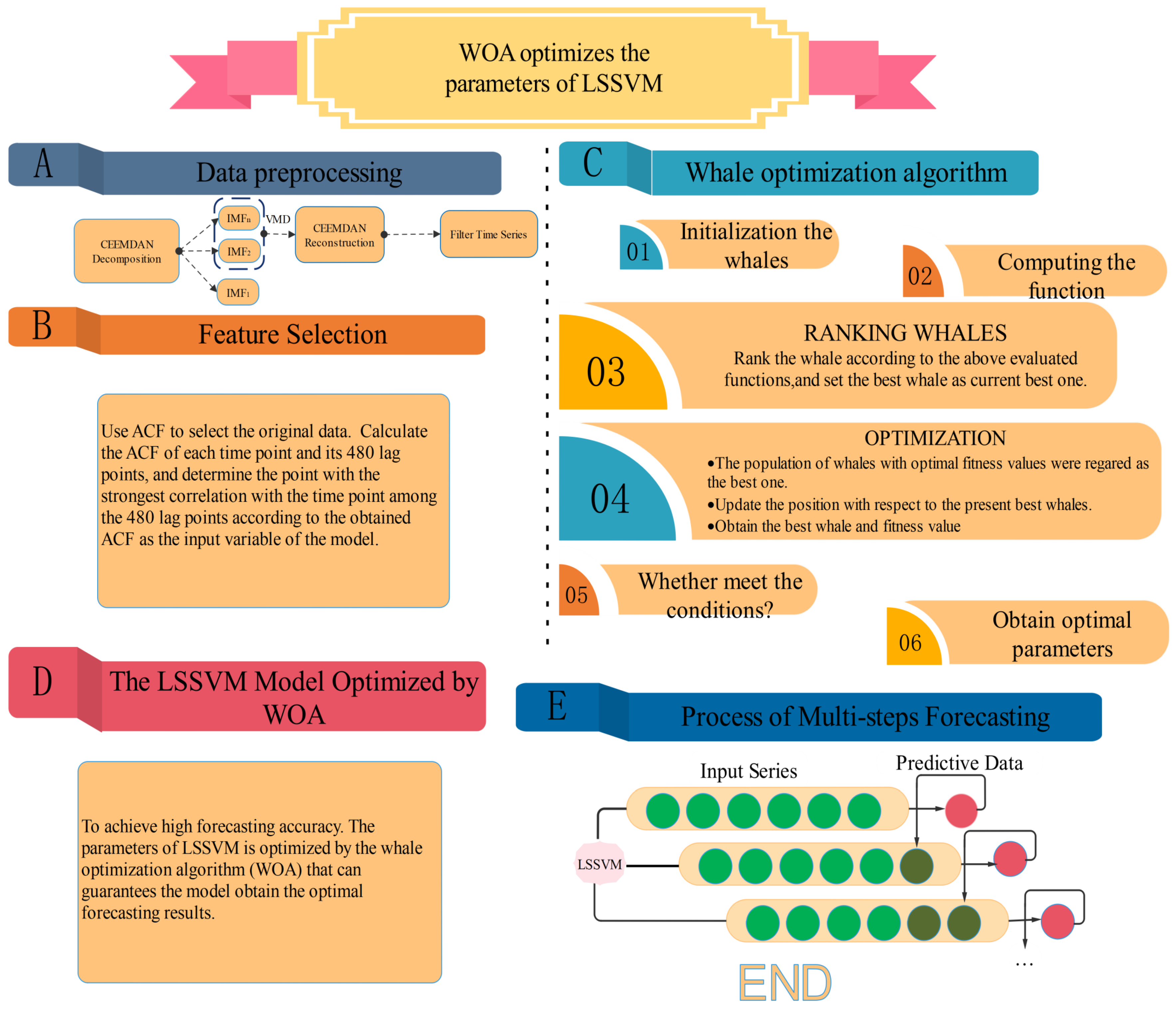
2.6. Lssvm Optimized by Woa

In order to overcome the shortcomings of the single algorithm and improve the accuracy and stability of the prediction, this section uses the new optimization algorithm WOA to optimize the parameters of the LSSVM, its pseudo code is shown in Algorithm 1. The informative descriptions of the hybrid WOA-LSSVM model can be given as the following steps.

• Initialize the parameters of the WOA and determine the objective function Equation (5)

  $$Fitness=\frac{1}{M}\sum _{i=1}^M{({\widehat{y}}_i-y_i)}^2$$

  (5)

  where M is the number of samples, $y_i$ and ${\widehat{y}}_i$ are the observed and predictive values of $P{M}_{2.5}$, respectively.
• Using WOA to iteratively optimize the parameters of LSSVM;
• See if the maximum iteration or preset error is met. If yes, run 4; Otherwise, continue to run 2;
• Set the optimal value obtained by WOA to c and ${\sigma }^2$ of LSSVM. Finally, the preprocessed data are used as the input of LSSVM to obtain the predicted value ${\widehat{y}}_i$.

Algorithm 1 WOA-LSSVM: optimize the parameters c and g of LSSVM with WOA.

Input:   $x_p^0=(x_{(1)}^0,x_{(2)}^0,\cdots ,x_{(q)}^0)$-the training time series   $x_p^0=(x_{(q+1)}^0,x_{(q+2)}^0,\cdots ,x_{(q+d)}^0)$-the testing time series Output:   ${\widehat{y}}_z^0=({\widehat{y}}_{(q+1)}^0,{\widehat{y}}_{(q+2)}^0,\cdots ,{\widehat{y}}_{(q+d)}^0)$-the forecasting data   LSSVM   Parameters   $Ite{r}_{Max}$-the maximum number of iterations   n-the number of whales   ${\mathbf{F}}_i$-the fitness function of i-th whale   ${\mathit{x}}_i$-the position of i-th whale   $it$-current iteration number   dim-the number of dimension.   /*Set the parameters of WOA.*/   /*Initilize population of n whale ${\mathit{x}}_i(i=1,2\cdots n)$randomly.*/   if $1\le i\le n$ then    Evaluate the corresponding fitness function ${\mathit{F}}_i$   end if   while $it<Ite{r}_{Max}$ do    for each $i=1:n$ do     for each $j=1:dim(n)$ do      Update a,A,C,l and p      if $p<0.5$ then       $D=|C·X^{*}(t)-X(t)|$       if $\left|A\right|<1$ then        /*Update the position of the current search agent.*/        $X_{t+1}=X_{rand}-A·D$       else        Select a random search agent($X_{rand}$)        /*Update the position of the current search agent.*/        $X_{t+1}=X_t^{*}-A·D$       end if      else       /*Update the position of the current search agent.*/       $X_{t+1}=D^{\prime }·e^{bl}·cos(2\pi l)+X^{*}(t)$      end if     end for    end for    /*Check if any search agent goes beyond the search space and amend it*/    for each $1\le i\le n$ do     Calculate fitness values of each search agent $F_i$    end for    /*Update the best search agent ${\mathit{X}}^{*}$.*/    $t=t+1$   end while   return $X^{*}$   Set parameters of LSSVM according to ${\mathit{X}}^{*}$   Use $x_t$ to train the LSSVM and update the parameters of the LSSVM   Input the historical data into LSSVM to obtain the forecasting value $\widehat{y}$.

3. Data Collection and Experimental Analysis

In order to verify the performance of the hybrid prediction model developed, two experiments are conducted in this section, and related experimental datasets, evaluation indicators and experimental designs are introduced.

3.1. Data Description

Data sets from two locations in Beijing and Yibin, China, were used to verify the performance of the proposed model. Beijing (${116}^{\circ }$ E, ${40}^{\circ }$ N) is located in northern China with less rainfall and relatively poor air quality. Yibin (${104.62}^{\circ }$ E, ${28.77}^{\circ }$ N) is located in central China with adequate rainfall and good air quality. The curves of original $P{M}_{2.5}$ concentrations data in the two areas are shown in Figure 2. It can be seen from Figure 2 that the $P{M}_{2.5}$ concentration values in the two regions have significant differences, but all have periodicity. Using the $P{M}_{2.5}$ data from these two places to verify the performance of the model is more representative. These two data sets are the data of $P{M}_{2.5}$ per hour from 5 January 2015 to 26 April 2015, a total of 2688, of which the first 2520 are used as training sets. After features selection, choose seven of the most relevant data used as model inputs to predict $P{M}_{2.5}$ concentrations at 168 points in the next week. See

Table 1. The basic statistics information of the $P{M}_{2.5}$ raw data in Beijing and Yibin of China.

Data Sets	Time	Training Days	Testing Days	Numbers	Means	min.	max.	std.
Beijing	1 h	5 January–19 April 2015	20 April–26 April 2015	2688	85.67	4	439	75.36
Yibin	1 h	5 January–19 April 2015	20 April–26 April 2015	2688	55.23	2	169	32.22

for basic information on the data sets.

3.2. Performance Estimation

In this subsection, five common performance criteria of forecast accuracy including absolute error (AE), mean absolute error (MAE), mean square error (MSE), and mean absolute percent error (MAPE), as well as IA are all listed in

Table 2. Five error metrics.

Metric	Definition	Equation
$IA$	The index of agreement of forecasting results	$IA=1-\frac{{\sum }_{i=1}^N{(y_i-{\widehat{y}}_i)}^2}{{\sum }_{i=1}^N(|{\widehat{y}}_i-\overline{y}|+|y_i-\overline{y}{|)}^2}$
$AE$	The average forecasting error	$AE=\frac{1}{N}{\sum }_{i=1}^N(y_i-{\widehat{y}}_i)$
$MAE$	The mean absolute forecasting error	$MAE=\frac{1}{N}{\sum }_{i=1}^N|y_i-{\widehat{y}}_i|$
$MSE$	Average of prediction error squares	$MSE=\frac{1}{N}{\sum }_{i=1}^N{(y_i-{\widehat{y}}_i)}^2$
$MAPE$	Mean Absolute Percentage Error	$MAPE=\frac{1}{N}{\sum }_{i=1}^N\left|\frac{y_i-{\widehat{y}}_i}{y_i}\right|\times 100\%$

, where N is the number of test samples, $y_i$ and ${\widehat{y}}_i$ represent the i-th observed and predicted values, respectively. In addition, $\overline{y}$ is the average value of the sample. Moreover, the roles of these error metrics can be listed as follows. AE can reflect positive and negative errors between predicted and observed values; Conversely, MAE is the mean absolute error, which can reflect the level of error. MSE is the average of the prediction error squares, which can be applied for estimating the change of forecasting models; MAPE is a measure of the prediction accuracy of a forecasting method in statistics; IA is also a useful measure of model performance allowing sensitivity to differences in observed and predicted sequences, as well as proportionality changes [50].

3.3. Testing Method

Although the above-mentioned methods have recognized the importance in assessing forecasting performance, statistical tests are used to assess the forecasting performance of a model from a statistical perspective. At present, the main statistical test methods mainly include parameter test [50] and non-parametric test [51,52]. As a type of parameter test, DM [50] test is often used to test prediction accuracy.

The hypothesis tests are Equations (6) and (7):

$$H_0:E(d_i)=0,\forall i$$

(6)

$$H_1:E(d_i)\ne 0,\exists i$$

(7)

The DM test statistic values equal (Equation (8)):

$$DM=\frac{\overline{D}}{\sqrt{S^2/N}}{s}^2$$

(8)

where ${\epsilon }_i$ denotes the forecast error, N denotes the total number of predicted samples, $\overline{D}$ denotes the mean of $d_i=L({\epsilon }_i^A)-L({\epsilon }_i^B)$, $S^2$ denotes an estimation value for the variance of $d_i$, and L denotes the loss function, which is performed to measure the forecasting accuracy. Here, the loss function we use is the square error loss.

The test statistic DM is convergent to the standard normal distribution. The null hypothesis will be rejected if, as shown in Equation (9):

$$\parallel DM\parallel >z_{\alpha /2}$$

(9)

where $\alpha /2$ is the critical z-value and $\alpha$ is the significance level.

3.4. Experimental Setup

In order to validate the newly proposed model, two experiments are set up for comparative analysis. Firstly, Experiment I analyzes the newly proposed model VCEEMDAN-SF-WOA-LSSVM longitudinally by comparing with seven benchmark models to elaborate on the advantages of the newly proposed model. Then, Experiment II is designed to compare with better previous models made in the prediction of $P{M}_{2.5}$ concentration (VCEEMDAN-SF-CS-LSSVM, VCEEMDAN-SF-BPNN, VCEEMDAN-SF-GRNN, VCEEMDAN-CS-LSSVM [53], VCEEMDAN-BPNN [22,54], VCEEMDAN-GRNN (Zhou Q. et al. 2014) [39], BPNN, GRNN, ARIMA [55]). It is found that after the feature selection, only a small number of input features can be selected to obtain higher prediction accuracy, and it is also found that WOA used in our model is better than some other meta-heuristic optimization algorithms such as CS in $P{M}_{2.5}$ concentration prediction.

4. Results

4.1. Experimental I

In this subsection, the performance of the newly proposed model is verified by comparing the seven models (SF-WOA-LSSVM, VCEEMDAN-WOA-LSSVM, VCEEMDAN-SF-LSSVM, VCEEMDAN-LSSVM, WOA-LSSVM, SF-LSSVM and LSSVM), as the benchmark models with the newly proposed model on the two data sets of $P{M}_{2.5}$ concentration in Beijing and Yibin. The forecasting results are shown in

Table 3. Experiment I forecasting results in Beijing.

Model	AE	MAE	MSE	MAPE (%)	IA
VCEEMDAN-SF-WOA-LSSVM	−0.9931	5.4957	57.7116	11.34	0.9803
SF-WOA-LSSVM	−0.8994	5.6535	60.5557	11.65	0.9792
VCEEMDAN-WOA-LSSVM	0.1008	11.2102	226.1804	20.17	0.9151
VCEEMDAN-SF-LSSVM	−0.4904	6.0393	67.2461	13.01	0.9774
VCEEMDAN-LSSVM	−0.3252	15.1042	404.6517	27.73	0.8412
LSSVM	−0.3110	15.1609	407.8657	27.78	0.8409

and

Table 4. Experiment I forecasting results in Yibin.

Model	AE	MAE	MSE	MAPE (%)	IA
SF-WOA-LSSVM	0.0784	2.0839	9.5472	6.40	0.9932
VCEEMDAN-WOA-LSSVM	0.08	4.1267	28.6088	13.34	0.9788
VCEEMDAN-SF-LSSVM	0.1905	2.5544	14.2633	7.85	0.9898
VCEEMDAN-LSSVM	0.2954	5.8399	56.9245	19.18	0.9570
LSSVM	0.3266	5.8170	56.3109	19.39	0.9575

. According to the results of eight different prediction models in Table 3 and Table 4, it can be seen that the developed prediction model not only has high prediction performance (measured by error criteria), but also achieves the highest accuracy in direction measurement (IA). Therefore, we can conclude that our hybrid prediction model based on feature selection (SF) and WOA is more suitable for $P{M}_{2.5}$ concentration than the other seven models that do not use these techniques.

4.1.1. Feature Selection

The results of PACF feature selection in the Beijing data set are shown in Figure 3. It can be seen from Figure 3 that the most severe lag variable is the first-order lag variable, and the partial correlation coefficient reaches 0.9822. Next is the second-order lag variable, and its partial correlation coefficient drops to 0.5358. Figure 3b shows the PACF score for 480 lag variables, but only the first 34 lag variables exceed the minimum limit. Since, ranking from large to small, the seventh absolute value of the partial correlation coefficient has dropped to 0.0686, and the partial correlation is already very weak. Therefore, we choose the first seven lag variables with higher partial correlation. They are lag1, lag2, lag3, lag64, lag65, lag4 and lag24.

The results and process of ACF feature selection in Beijing are shown in Figure 4. Figure 4a shows the autocorrelation values of the initial candidate variables in Beijing. We can see that the first linear correlation is the strongest and the others are relatively weak. The strongest linear correlation is at lag1, and the second strongest is at lag2. Since the peak at lag1 is the highest, the first peak is important. We should choose the variable as the input variable. In addition, the ACF graph also reflects daily and weekly cycles, which ensures the importance of feature selection for predicting future $P{M}_{2.5}$ concentrations.

The results of the PACF feature selection in Yibin are shown in Figure 5. Figure 5a shows that the lag variable with the strongest partial correlation is the first-order lag variable, and its partial correlation coefficient reaches 0.9894. The second partial correlation is also strong, and the partial correlation coefficient is reduced to 0.6511. The third one with strong partial correlation is the third-order lag variable, and the partial correlation coefficient is 0.1098. Figure 5b shows the PACF score for 480 lag features, but only the first 45 lag variables exceed the limit. Because, from large to small, the sixth of the absolute value of the partial correlation coefficient has dropped to 0.0881, and the partial correlation becomes weak after that. Therefore, we choose the top 8 lag variables with higher partial correlation than the input variables. They are lag1, lag2, lag3, lag4, lag17, lag8, lag6 and lag15, respectively.

The results and process of ACF feature selection in Yibin are shown in Figure 6. Figure 6a shows the autocorrelation values of the initial candidate variables in Yibin. We can see that Yibin’s data are relatively stable. The first linear correlation is the strongest, and the others are relatively weak. Similarly, the strongest linear correlation is at lag1, and the linear correlation of the second strongest is at lag2. Since the peak at hysteresis 1 is the highest, this means that the first peak is very important, which suggests that we should choose the variable as the input variable.

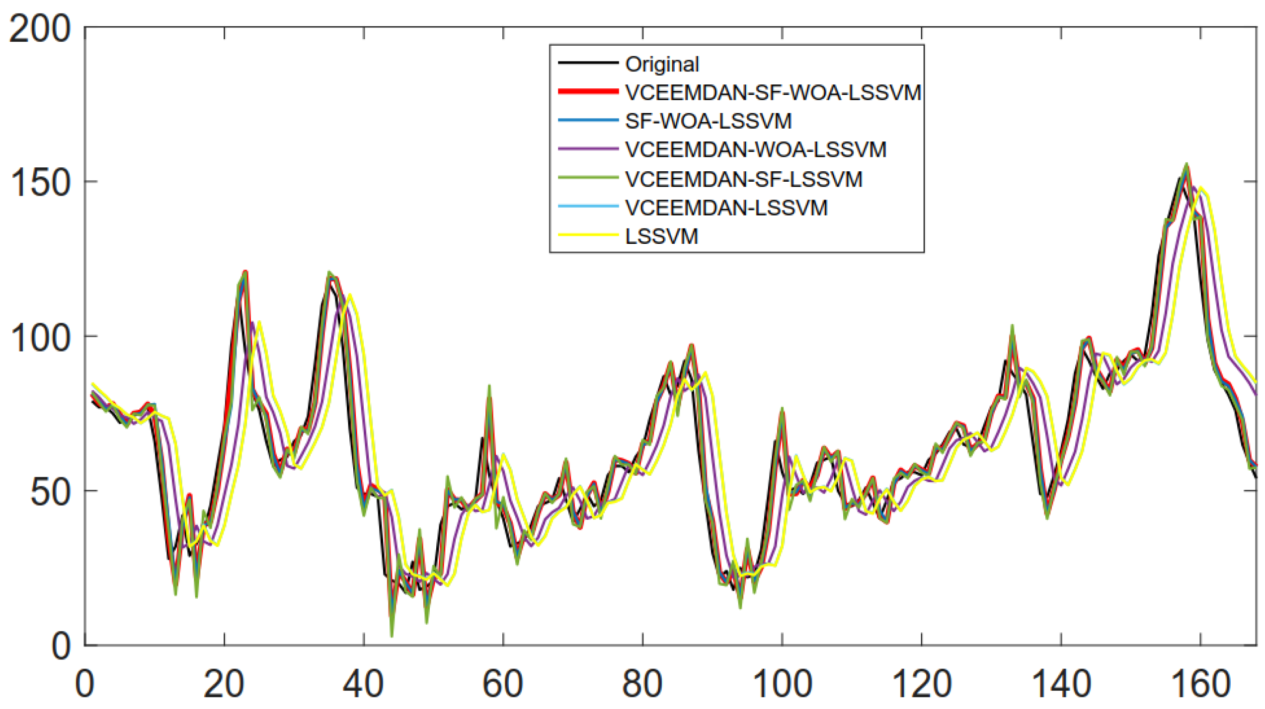
4.1.2. Forecast Results and Analysis

In order to show the efficiency of the newly proposed model, we remove some modules to construct some comparing models to predict the concentration of $P{M}_{2.5}$ in Beijing and Yibin in the coming week. The prediction results of Beijing are shown in Figure 7. We can see that the prediction curve of our new model basically goes to the original data curve. The specific evaluation results are shown in Table 3. It can be seen from Table 3 that the proposed model VCEEMDAN-SF-WOA-LSSVM has a prediction accuracy metric of 11.34 on MAPE, which is far lower than that of other models. In addition, its accuracy is improved 43.77% compared with that of VCEEMDAN-WOA-LSSVM without feature selection. In addition, by comparing the newly proposed model with SF-WOA-LSSVM, it is found that the denoising procession of the original data has a certain improvement on the prediction accuracy, but the improvement effect is not particularly obvious. Furthermore, the results of the newly proposed model and VCEEMDAN-SF-LSSVM show that the optimization algorithm WOA has a large impact on the model prediction. After using WOA, the prediction accuracy of the model is improved by 12.84%. Finally, compared with the prediction results of the newly proposed model and VCEEMDAN-LSSVM, the evaluation index MAPE is increased by 59.11%, which is enough to prove the high importance of feature selection and optimization algorithms for model prediction results.

The prediction results of Yibin are shown in Figure 8. We can see that the prediction results of our newly proposed model are basically coincident with the real data. The specific evaluation results are shown in Table 4. It can be seen from the quantitative prediction indicators that our newly proposed model is quite accurate for the prediction of 168 data points in the next week, and its MAPE reaches 6.15, which is higher than the prediction accuracy of the models proposed in the existing literature. IA is the indicator of consent for the predictions, which is better when it is close to 1. We can see that the IA of our proposed model has reached 0.9940, which means that our new model is very suitable for predicting $P{M}_{2.5}$ concentration. For MAPE, our proposed model VCEEMDAN-SF-WOA-LSSVM is improved 3.91%, 53.90%, 21.65%, 67.94% and 68.28% compared with the models SF-WOA-LSSVM, VCEEMDAN-WOA-LSSVM, VCEEMDAN-SF-LSSVM, VCEEMDAN-LSSVM and LSSVM, respectively. It can be seen that the benchmark models corresponding to several MAPEs with larger amplitudes do not adopt feature selection techniques or optimization algorithms. Thus, the accuracy of the feature selection and optimization algorithm for model prediction is further reflected.

The statistical test results of Experiment I are shown in

Table 5. Results of DM test for Experiment I.

Compared Models	Beijing		Yibin
	DM-Value	p-Value	DM-Value	p-Value
VCEEMDAN-SF-WOA-LSSVM vs. SF-WOA-LSSVM	2.984	0.000 **	5.714	0.000 **
VCEEMDAN-SF-WOA-LSSVM vs. VCEEMDAN-WOA-LSSVM	6.167	0.000 **	2.935	0.002 **
VCEEMDAN-SF-WOA-LSSVM vs. VCEEMDAN-SF-LSSVM	2.769	0.000 **	6.877	0.000 **
VCEEMDAN-SF-WOA-LSSVM vs. VCEEMDAN-LSSVM	7.248	0.000 **	5.659	0.000 **
VCEEMDAN-SF-WOA-LSSVM vs. LSSVM	7.246	0.000 **	7.354	0.000 **

** represents that the test indicates not to accept the null hypothesis under $\alpha =0.025$.

. As can be seen from Table 5, the p-value of VCEEMDAN-SF-WOA-LSSVM and VCEEMDAN-WOA-LSSVM is less than 0.025. Therefore, we have a probability of greater than 95% to reject the null hypothesis, and there is a significant difference between the two models. This result demonstrates once again the importance of feature selection from a statistical perspective. When throwing away WOA, the p-value of comparing models VCEEMDAN-SF-WOA-LSSVMA and VCEEMDAN-SF-LSSVM is also much less than 0.025, which reflects the importance of the optimization algorithm. Experiments show that our proposed hybrid model with feature selection and optimization algorithms has the best predictive performance and strong stability.

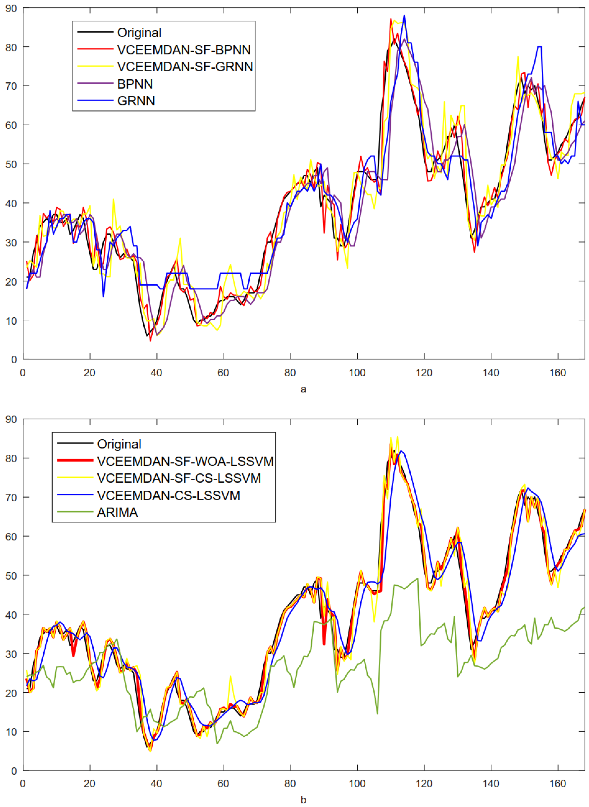
4.2. Experimental II

By comparing with some of the fine $P{M}_{2.5}$ prediction models, we conducted this experiment on the two completely different data sets to show that our newly proposed model (VCEEMDAN-SF-WOA-LSSVM) is superior to the best performing model for $P{M}_{2.5}$ prediction. The prediction results on Beijing data set are shown in Figure 9. It can be seen intuitively that our newly proposed model VCEEMDAN-SF-WOA-LSSVM fits best with real data, while the ARIMA is the worst in the comparison models. It can be seen from Figure 9a that after the feature selection, the prediction results modeled by BPNN and GRNN are greatly improved, which indicates the high importance of the feature selection in the modeling. It is found from Figure 9b that when the optimization algorithm WOA is replaced by CS, there is a significant difference between the prediction curve and the real value curve. The model’s predictive ability is even worse without feature selection. The quantitative evaluation indicators are shown in

Table 6. Experiment II forecasting results in Beijing.

Model	AE	MAE	MSE	MAPE (%)	IA
VCEEMDAN-SF-WOA-LSSVM	−0.9931	5.4957	57.7116	11.34	0.9803
VCEEMDAN-SF-CS-LSSVM	−0.6123	6.1817	69.5793	13.38	0.9766
VCEEMDAN-SF-BPNN	−0.3991	6.6083	75.8084	14.24	0.9746
VCEEMDAN-SF-GRNN	−4.1243	14.1117	313.2350	26.87	0.8962
VCEEMDAN-CS-LSSVM	−0.1054	11.4278	234.7603	20.46	0.9125
BPNN	−2.5047	17.2058	556.2312	32.46	0.7997
GRNN	3.3690	12.0000	258.2738	22.77	0.9012
ARIMA	−6.9863	16.6792	490.1992	39.44	0.6893

. It can be seen that when the optimization algorithm is replaced by the cuckoo optimization algorithm (CS), the MAPE value increases to 13.38, which means that the optimization algorithm WOA performs better than CS, meaning it is more suitable for prediction with $P{M}_{2.5}$ concentration. In addition, BPNN is also ideal for predicting $P{M}_{2.5}$ concentration. In particular, after adding the feature selection technique, the MAPE value is decreased by 56.13% comparing VCEEMDAN-SF-BPNN with BPNN, which is also illustrated in Figure 9a. Similarly, when using GRNN prediction, after adding feature selection, the MAPE value is increased by 38.42%. In general, the MAPE value of our newly proposed model VCEEMDAN-SF-WOA-LSSVM is improved by 15.24%, 60.54%, 46.31%, 65.06%, 50.19% and 71.25%, compared with that of the model VCEEMDAN-CS-LSSVM, VCEEMDAN-BPNN, VCEEMDAN-GRNN, BPNN, GRNN and ARIMA respectively.

The prediction results on Yibin data set are shown in Figure 10 and Table 6. As can be seen from Figure 10, the ARIMA model is still the worst prediction, which further indicates that the linear model is not suitable for the prediction of $P{M}_{2.5}$ concentration. Our new model is much more effective than other models. Figure 10a again demonstrates the high performance of feature selections. It can be found from Figure 10b that the model prediction curves with feature selection technology and WOA are near the real data curve, which further confirms the high performance of feature selection technology and optimization algorithm. From

Table 7. Experiment II forecasting results in Yibin.

Model	AE	MAE	MSE	MAPE (%)	IA
VCEEMDAN-SF-WOA-LSSVM	0.0844	1.9688	8.4035	6.15	0.9940
VCEEMDAN-SF-CS-LSSVM	−0.0935	2.5581	13.2533	8.29	0.9905
VCEEMDAN-SF-BPNN	−0.2707	2.4995	13.5391	8.48	0.9903
VCEEMDAN-SF-GRNN	−0.1704	4.3682	32.0127	14.74	0.9778
VCEEMDAN-CS-LSSVM	0.0919	4.1194	28.4881	13.31	0.9789
BPNN	0.7761	6.0931	64.3302	20.06	0.9521
GRNN	−0.5357	5.9405	50.7738	22.31	0.9594
ARIMA	12.0946	16.5594	276.9223	35.05	0.7300

, it can be seen that the MAPE values of the first four models added with feature selection are lower than 15, which fully indicates the importance of feature selection technology to the prediction results. Finally, the MAPE value of our newly proposed model VCEEMDAN-SF-WOA-LSSVM for the prediction accuracy of $P{M}_{2.5}$ concentration in Yibin in the next week reached 6.15, far lower than the other seven benchmark models, and it is the model with the best predicted performance so far.

Table 8. Results of DM test for Experiment II.

Compared Models	Beijing		Yibin
	DM-Value	p-Value	DM-Value	p-Value
VCEEMDAN-SF-WOA-LSSVM vs. VCEEMDAN-SF-CS-LSSVM	3.034	0.000 **	3.636	0.009 **
VCEEMDAN-SF-WOA-LSSVM vs. VCEEMDAN-SF-BPNN	2.928	0.004 **	3.843	0.000 **
VCEEMDAN-SF-WOA-LSSVM vs. VCEEMDAN-SF-GRNN	7.697	0.000 **	5.719	0.000 **
VCEEMDAN-SF-WOA-LSSVM vs. VCEEMDAN-CS-LSSVM	6.246	0.000 **	5.952	0.000 **
VCEEMDAN-SF-WOA-LSSVM vs. BPNN	6.588	0.000 **	6.458	0.000 **
VCEEMDAN-SF-WOA-LSSVM vs. GRNN	5.167	0.000 **	8.839	0.000 **
VCEEMDAN-SF-WOA-LSSVM vs. ARIMA	7.097	0.000 **	9.992	0.000 **

** represents that the test indicates not to accept the null hypothesis under $\alpha =0.025$.

is the statistical test results of the proposed model and the benchmark models. It can be seen from Table 8 that after replacing the WOA with CS, the performance of the two models on the two data sets both have significant difference, which indicates that the optimization performance of WOA is better than that of CS in the prediction of $P{M}_{2.5}$. From the comparison of VCEEMDAN-SF-WOA-LSSVM vs. VCEEMDAN-SF-BPNN, VCEEMDAN-SF-WOA-LSSVM vs. VCEEMDAN-SF-GRNN, VCEEMDAN-SF-WOA- LSSVM vs. BPNN and VCEEMDAN-SF-WOA-LSSVM vs. GRNN, it is found that the the p-values are all minus 0.05, which indicate that there are significant differences between the compared models. By comparing with the evaluation indicators, we can conclude that our proposed model has better forecasting performance in terms of $P{M}_{2.5}$ prediction.

5. Conclusions and Future Study

This paper proposes a new combined LSSVM-based forecasting model, by combining CEEMDAN, VMD, SF and WOA algorithms with LSSVM model, namely VCEEMDAN-SF-WOA-LSSVM. In the empirical study of two different perspectives of Experiment I and Experiment II, the proposed model has achieved the best prediction results compared with other single AI models and hybrid models. To overcome the inherent shortcomings of LSSVM parameter selection, a new optimization algorithm (WOA) is adopted for parameter optimization. By taking feature selection, the input variables are chosen to build the model, which makes the operation time of the whole model faster and the operating cost lower. Finally, the proposed VCEEMDAN-SF-WOA-LSSVM model is used on two data sets to achieve significant prediction accuracy.

The most important contribution of the research is the newly proposed hybrid model, which can be used on accurate $P{M}_{2.5}$ prediction. Some interesting findings are also worth stating here. Firstly, for the great influence of the model parameters c and ${\sigma }^2$ on the prediction effect, using a group intelligent optimization algorithm to optimize the parameters of LSSAM is a good idea. This paper combines the powerful optimization ability of WOA with the good prediction performance of LSSVM, thus further reducing the prediction error of the model. Secondly, in view of the shortcomings of the general combined model, such as slow running time and high cost, the feature engineering method to reduce the number of input variables is used, which reduces the operation time and calculation cost of the whole model. Finally, it can be found that the proposed model can do automatic prediction if the computer’s computing ability allows it. As long as the corresponding raw data are given, our model can automatically find the highly relevant variables as input variables, and automatically predict, without manual intervention. In other words, our model VCEEMDAN-SF-WOA-LSSVM is a fully automated machine learning model.

$P{M}_{2.5}$ prediction is very useful for human health and environment management, but it is a challenging job. Abandoning the traditional linear model, noting that the nonlinear relationship exists inside the data time series, thus nonlinear fitting is the necessary choice of prediction. However, the factors causing $P{M}_{2.5}$ are extremely complex, including geographical factors, climate, temperature, rainfall, humidity, etc., predicting the concentration of $P{M}_{2.5}$ based solely on historical data will inevitably affect the accuracy of the forecast. Therefore, people can consider starting from the $P{M}_{2.5}$ generation process, and taking into account various factors causing the increase of $P{M}_{2.5}$ in future research. In other words, studying how to explore suitable and reasonable components to build a model may be the future research direction. In addition, although our model achieves the best prediction accuracy so far, it requires higher computer spending and longer training time than a single model. However, with the rapid development of computers, this problem has now been overcome. Finally, an interesting potential direction is to further improve and optimize performance using this new hybrid model on other complex real problems.

References

1. Chen, W. Urban air quality evaluations under two versions of the national ambient air quality standards of China. Atmos. Pollut. Res. 2016, 7, 49–57. [Google Scholar] [CrossRef]
2. Ye, W.F. Spatial-temporal patterns of PM2.5 concentrations for 338 Chinese cities. Sci. Total. Environ. 2018, 631–632, 524–533. [Google Scholar] [CrossRef] [PubMed]
3. Wang, Y. Air quality assessment by contingent valuation in Ji’nan, China. J. Environ. Manag. 2009, 90, 1022–1029. [Google Scholar] [CrossRef] [PubMed]
4. Zhang, H.; Wang, S.; Hao, J. Air pollution and control action in Beijing. J. Clean. Prod. 2016, 112, 1519–1527. [Google Scholar] [CrossRef]
5. Zheng, S. The impacts of provincial energy and environmental policies on air pollution control in China. Renew. Sustain. Energy Rev. 2015, 49, 386–394. [Google Scholar] [CrossRef]
6. Chen, T.F. Modeling direct and indirect effect of long range transport on atmospheric PM2.5, levels. Atmos. Environ. 2014, 89, 1–9. [Google Scholar] [CrossRef]
7. Fang, G.C.; Chang, C.N.; Wang, N.P. The study of TSP, PM2.5–10, and PM2.5, during Taiwan Chi-Chi Earthquake in the traffic site of central Taiwan, Taichung. Chemosphere 2000, 41, 1727–1731. [Google Scholar] [CrossRef]
8. Chudnovsky, A.A.; Koutrakis, P.; Kloog, I. Fine particulate matter predictions using high resolution Aerosol Optical Depth(AOD) retrievals. Atmos. Environ. 2014, 89, 189–198. [Google Scholar] [CrossRef]
9. Shen, F.; Ge, X.; Hu, J. Air pollution characteristics and health risks in Henan Province, China. Environ. Res. 2017, 156, 625–634. [Google Scholar] [CrossRef]
10. You, W.; Zang, Z.; Pan, X. Estimating PM2.5 in Xi’an, China using aerosol optical depth: A comparison between the MODIS and MISR retrieval models. Sci. Total. Environ. 2015, 505, 1156–1165. [Google Scholar] [CrossRef] [PubMed]
11. Scapellato, M.L.; Canova, C.; Simone, A.D. Personal PM10 exposure in asthmatic adults in Padova, Italy: seasonal variability and factors affecting individual concentrations of particulate matter. Int. J. Hyg. Environ. Health 2009, 212, 626–636. [Google Scholar] [CrossRef] [PubMed]
12. Niu, M.; Wang, Y.; Sun, S. A novel hybrid decomposition-and-ensemble model based on CEEMD and GWO for short-term PM2.5, concentration forecasting. Atmos. Environ. 2016, 134. [Google Scholar] [CrossRef]
13. Kukkonen, J.; Partanen, L.; Karppinen, A. Extensive evaluation of neural network models for the prediction of NO and PM10 concentrations, compared with a deterministic modelling system and measurements in central Helsinki. Atmos. Environ. 2003, 37, 4539–4550. [Google Scholar] [CrossRef]
14. Turner, M.C.; Krewski, D.; Pope, C.A. Long-term ambient fine particulate matter air pollution and lung cancer in a large cohort of never-smokers. Am. J. Respir. Crit. Care Med. 2011, 184, 1374–1381. [Google Scholar] [CrossRef] [PubMed]
15. Gu, K. Highly efficient picture-based prediction of PM2.5 concentration. IEEE Trans. Ind. Electron. 2018, 99, 1. [Google Scholar] [CrossRef]
16. Zhai, B.; Chen, J. Development of a stacked ensemble model for forecasting and analyzing daily average PM2.5, concentrations in Beijing, China. Sci. Total. Environ. 2018, 635, 644–658. [Google Scholar] [CrossRef]
17. Yufang, W.; Haiyan, W.; Shuhua, C. Prediction of daily PM2.5 concentration in China using partial differential equations. PLoS ONE 2018, 13, e0197666. [Google Scholar]
18. Stella, M. A dynamic multiple equation approach for forecasting PM2.5 pollution in Santiago, Chile. Int. J. Forecast. 2018, 34, 566–581. [Google Scholar]
19. Junxiong, H.; Qi, L.I.; Yajie, Z. Real-time forecasting system of PM2.5 concentration based on spark framework and random forest model. Sci. Surv. Mapp. 2017, 42, 1–6. [Google Scholar] [CrossRef]
20. Yichao, L.; Lu, X.; Christakos, G. Forecasting concentrations of PM2.5 in main urban area of Hangzhou and mapping using SARIMA model and ordinary Kringing method. Acta Sci. Circumstantiae 2018, 38, 62–70. [Google Scholar] [CrossRef]
21. Cobourn, W.G. An enhanced PM2.5 air quality forecast model based on nonlinear regression and back-trajectory concentrations. Atmos. Environ. 2010, 44, 3015–3023. [Google Scholar] [CrossRef]
22. Bai, Y.; Li, Y.; Wang, X. Air pollutants concentrations forecasting using back propagation neural network based on wavelet decomposition with meteorological conditions. Atmos. Pollut. Res. 2016, 7, 557–566. [Google Scholar] [CrossRef]
23. Biancofiore, F.; Busilacchio, M.; Verdecchia, M. Recursive neural network model for analysis and forecast of PM10 and PM2.5. Atmos. Pollut. Res. 2017, 8, 652–659. [Google Scholar] [CrossRef]
24. Díaz-Robles, L.A.; Ortega, J.C.; Fu, J.S.; Reed, G.D.; Chow, J.C.; Watson, J.G.; Moncada-Herrera, J.A. A hybrid ARIMA and artificial neural networks model to forecast particulate matter in urban areas: The case of Temuco, Chile. Atmos. Environ. 2008, 42, 8331–8340. [Google Scholar] [CrossRef] [Green Version]
25. Prakash, A.; Kumar, U.; Kumar, K. A Wavelet-based Neural Network Model to Predict Ambient Air Pollutants’ Concentration. Environ. Model. 2011, 16, 503–517. [Google Scholar] [CrossRef]
26. Lv, B.; Cobourn, W.G.; Bai, Y. Development of nonlinear empirical models to forecast daily PM2.5, and ozone levels in three large Chinese cities. Atmos. Environ. 2016, 147, 209–223. [Google Scholar] [CrossRef]
27. Sun, W.; Zhang, H.; Palazoglu, A. Prediction of 24-Hour-Average PM2.5 Concentrations Using a Hidden Markov Model with Different Emission Distributions in Northern California. Sci. Total. Environ. 2012, 443, 93–103. [Google Scholar] [CrossRef]
28. Shenru, X.; Binbin, Q.; Baohua, Y. Influence on Input Parameters of PM2.5 Concentration Prediction Model Based on LIBSVM. J. Luoyang Inst. Sci. Technol. 2017, 27, 9–12. [Google Scholar] [CrossRef]
29. Zhu, S.; Lian, X.; Wei, L. PM2.5 forecasting using SVR with PSOGSA algorithm based on CEEMD, GRNN and GCA considering meteorological factors. Atmos. Environ. 2018, 183. [Google Scholar] [CrossRef]
30. Paschalidou, A.K.; Karakitsios, S.; Kleanthous, S. Forecasting hourly PM10 concentration in Cyprus through artificial neural networks and multiple regression models: implications to local environmental management. Environ. Sci. Pollut. Res. 2011, 18, 316–327. [Google Scholar] [CrossRef]
31. Feng, X.; Li, Q.; Zhu, Y. Artificial neural networks forecasting of PM2.5, pollution using air mass trajectory based geographic model and wavelet transformation. Atmos. Environ. 2015, 107, 118–128. [Google Scholar] [CrossRef]
32. Feng, S.; Wengao, L.; Bo, Z. Neural network model for PM2.5 concentration prediction by grey wolf optimizer algorithm. J. Comput. Appl. 2017, 37, 2854–2860. [Google Scholar] [CrossRef]
33. Yali, F.U.; Ya, H. Air Quality Forecasting Based on IPSO-ELM. Environ. Sci. Technol. 2017, 40, 324–328. [Google Scholar]
34. Liming, W.; Xianghua, W.U.; Tianliang, Z. A scheme for rolling statistical forecasting of PM2.5 concentrations based on distance correlation coefficient and support vector regression. Acta Sci. Circumstantiae 2017, 37, 1268–1276. [Google Scholar] [CrossRef]
35. Lijie, D.; Changjiang, Z.; Leiming, M.A. Dynamic forecasting model of short-term PM2.5 concentration based on machine learning. J. Comput. Appl. 2017, 37, 3057–3063. [Google Scholar] [CrossRef]
36. Gan, K.; Sun, S.; Wang, S. A secondary-decomposition-ensemble learning paradigm for forecasting PM2.5, concentration. Atmos. Pollut. Res. 2018, 9, 989–999. [Google Scholar] [CrossRef]
37. García Nieto, P.J.; Sánchez Lasheras, F.; Garcxixa-Gonzalo, E.; de Cos Juez, F.J. PM10, concentration forecasting in the metropolitan area of Oviedo (Northern Spain) using models based on SVM, MLP, VARMA and ARIMA: A case study. Sci. Total. Environ. 2018, 621, 753–761. [Google Scholar] [CrossRef]
38. Gualtieri, G. Forecasting PM10, hourly concentrations in northern Italy: Insights on models performance and PM10, drivers through self-organizing maps. Atmos. Pollut. Res. 2018. [Google Scholar] [CrossRef]
39. Zhou, Q.; Jiang, H.; Wang, J. A hybrid model for PM2.5, forecasting based on ensemble empirical mode decomposition and a general regression neural network. Sci. Total. Environ. 2014, 496, 264–274. [Google Scholar] [CrossRef]
40. Weide, L.; Demeng, K.; Jinran, W. A New Hybrid Model FPA-SVM Considering Cointegration for Particular Matter Concentration Forecasting: A Case Study of Kunming and Yuxi, China. Comput. Intell. Neurosci. 2017, 366, 1–11. [Google Scholar] [CrossRef]
41. Ping, J. A novel hybrid strategy for PM2.5, concentration analysis and prediction. J. Environ. Manag. 2017, 196, 443–457. [Google Scholar] [CrossRef]
42. Liu, B. Forecasting PM2.5 concentration using spatio-temporal extreme learning machine. In Proceedings of the 2016 15th IEEE International Conference on Machine Learning and Applications (ICMLA), Anaheim, CA, USA, 18–20 December 2016. [Google Scholar]
43. Li, X.; Peng, L.; Yao, X. Long short-term memory neural network for air pollutant concentration predictions: Method development and evaluation. Environ. Pollut. 2017, 231, 997–1004. [Google Scholar] [CrossRef]
44. Huang, N.E. The empirical mode decomposition and the Hilbert spectrum for nonlinear and non-stationary time series analysis. Proc. Math. Phys. Eng. Sci. 1998, 454, 903–995. [Google Scholar] [CrossRef]
45. Wu, Z. Ensemble empirical mode decomposition. Adv. Adapt. Data Anal. 2009, 1, 1e41. [Google Scholar]
46. María, E.; Colominas, M.A.; Schlotthauer, G.; Flandrin, P. A complete ensemble empirical mode decomposition with adaptive noise. In Proceedings of the 2011 IEEE International Conference on Acoustics, Speech and Signal Processing (ICASSP), Prague, Czech Republic, 22–27 May 2011; pp. 4144–4147. [Google Scholar]
47. Dragomiretskiy, K. Variational Mode Decomposition. IEEE Trans. Signal Process. 2014, 62, 531–544. [Google Scholar] [CrossRef]
48. Mirjalili, S.; Lewis, A. The Whale Optimization Algorithm. Adv. Eng. Softw. 2016, 95, 51–67. [Google Scholar] [CrossRef]
49. Du, P.; Wang, J.; Yang, W. Multi-step ahead forecasting in electrical power system using a hybrid forecasting system. Renew. Energy 2018, 122, 533–550. [Google Scholar] [CrossRef]
50. Wang, J. A novel hybrid system based on a new proposed algorithm - Multi - Objective Whale Optimization Algorithm for wind speed forecasting. Appl. Energy 2017, 208, 344–360. [Google Scholar] [CrossRef]
51. Dong, Y. A hybrid seasonal mechanism with a chaotic cuckoo search algorithm with a support vector regression model for electric load forecasting. Energies 2018, 11, 1009. [Google Scholar] [CrossRef]
52. Fan, G.F. Short term load forecasting based on phase space reconstruction algorithm and bi-square kernel regression model. Appl. Energy 2018, 224, 13–33. [Google Scholar] [CrossRef]
53. Sun, W. Daily PM2.5 concentration prediction based on principal component analysis and LSSVM optimized by cuckoo search algorithm. J. Environ. Manag. 2017, 188, 144–152. [Google Scholar] [CrossRef] [PubMed]
54. Deyun, W.; Yanling, L.; Hongyuan, L. Day-ahead PM2.5 concentration forecasting using WT-VMD based decomposition method and back propagation neural network improved by differential evolution. Int. J. Environ. Res. Public Health 2017, 14, 764. [Google Scholar] [CrossRef]
55. Mahajan, S.; Chen, L.J.; Tsai, T.C. Short-term PM2.5 forecasting using exponential smoothing method: A comparative analysis. Sensors 2018, 18, 3223. [Google Scholar] [CrossRef] [PubMed]
Figure 1. The flowchart and components of the proposed combined model to forecast P M 2.5 in the next week.
Atmosphere 10 00223 g001
Figure 2. Raw data in Beijing and Yibin, China.
Atmosphere 10 00223 g002
Figure 3. PACF for each time lag variable and ranked PACF in Beijing. (a): PACF for each time lag variable; (b): ranked PACF. The closer the value is to 1, the greater the partial correlation. Conversely, the closer the value is to 0, the smaller the partial correlation.
Atmosphere 10 00223 g003
Figure 4. ACF of time lag variables and ranked ACF result in Beijing. (a): ACF for each time lag variable; (b): ranked ACF. The closer the value is to 1, the greater the autocorrelation. Conversely, the closer the value is to 0, the smaller the autocorrelation.
Atmosphere 10 00223 g004
Figure 5. PACF for each time lag variable and ranked PACF in Yibin. (a): PACF for each time lag variable; (b): ranked PACF. Its understanding is similar to Figure 3.
Atmosphere 10 00223 g005
Figure 6. ACF of time lag variables and ranked ACF result in Yibin. (a): ACF for each time lag variable; (b): ranked ACF. Its understanding is similar to Figure 4.
Atmosphere 10 00223 g006
Figure 7. The forecast results of Beijing in the next week (20 April–26 April 2015): to highlight the prediction accuracy of the hybrid model comparing with the models without VCEEMDAN, SF or WOA.
Atmosphere 10 00223 g007
Figure 8. The forecast results of Yibin in the next week (20 April–26 April 2015): to highlight the prediction accuracy of the hybrid model comparing with the models without VCEEMDAN, SF or WOA.
Atmosphere 10 00223 g008
Figure 9. The forecast results in Beijing: (a) demonstrate the SF effects on general regression neural network (GRNN) and BP neural networks (BPNN) models and (b) illustrate the superiorities of SF and WOA in the proposed combined model.
Atmosphere 10 00223 g009
Figure 10. The forecast results in Yibin: (a) demonstrate the SF effects on GRNN and BPNN models and (b) illustrate the superiorities of SF and WOA in the proposed combined model.
Atmosphere 10 00223 g010