Article

Spatial Characteristics of Deep-Developed Boundary Layers and Numerical Simulation Applicability over Arid and Semi-Arid Regions in Northwest China

1
College of Atmospheric Sciences, Lanzhou University, Lanzhou 730000, China
2
College of Computer and Communication, Lanzhou University of Technology, Lanzhou 730050, China
*
Author to whom correspondence should be addressed.
Atmosphere 2019, 10(4), 195; https://doi.org/10.3390/atmos10040195
Submission received: 4 March 2019 / Revised: 28 March 2019 / Accepted: 9 April 2019 / Published: 11 April 2019
(This article belongs to the Section Meteorology)

Abstract

:
The spatial distribution and long-time variation of the deep-developed boundary layer are not well understood in arid and semi-arid regions of northwest China. ERA-Interim (ECMWF Reanalysis data, ECMWF: European Centre for Medium-Range Weather Forecasts) were used to study the deep-developed boundary layer in the five representative areas in summer and then the Weather Research Forecast (WRF) model was applied to simulate and verify its applicability. The results show that the boundary layer heights in the five representative areas are higher in late spring and summer (the highest is 2485~3502 m in June) and lower in autumn, winter and early spring (the lowest is 758~907 m in December). The seasonal variations of the boundary layer height are smaller at 02:00 BJT and 08:00 BJT, while the variations are relatively larger at 14:00 BJT and 20:00 BJT. The atmospheric boundary layer, with heights over 4000 m, generally exists in late spring and summer. The boundary layer heights are higher in the arid region than in the semi-arid region and the deep-developed boundary layer lasts longer in the arid region. The boundary layer heights present reductions from the northwest to the southeast, except for Minqin in the middle north. The numerical simulation results show that there is a significant difference between different combinations of parameterization schemes to simulate the deep-developed boundary layer in these areas. The combination Goddard+SLAB+ACM2 performs better in the extreme arid area, Dunhuang, and the arid areas, Jiuquan and Minqin, whereas the simulation effect of the combination Dudhia+Noah+ACM2 is better in the semi-arid areas, Yuzhong and Lanzhou. The difference between the schemes is related to the determination of the boundary layer height.

1. Introduction

The atmospheric boundary layer is connected to the surface and is an important intermediary for the rapid exchange of momentum, heat, moisture, and mass between free atmosphere and different underlying surfaces (such as soil, vegetation, water and ice). Some important weather phenomena, such as precipitation, fog and frost, are mostly closely related to the boundary layer development, especially for high-impact weather formation such as dust storms and heavy rains. The atmospheric boundary layer height is an important parameter to measure the boundary layer development, which plays a key role in the atmospheric environment capacity, aerosol distribution, convective activity and cloud formation in a certain region. As an index, it also determines processes of turbulence mixing, vertical diffusion, convection transport and atmospheric pollutant settlement. It is a key physical variable in models for numeric simulation. Usually, the height of the convective boundary layer during the day is generally 1000–2000 m, and the stable boundary layer at night is does not exceed 400–500 m [1,2]. However, the atmospheric boundary layer develops highly in special climate conditions due to geographical environment influences. For example, the development of the atmospheric boundary layer is different from the general defined height, especially in arid and semi-arid regions for the low surface vegetation coverage. It leads to significantly high transports of mass and energy between the surface and atmosphere. Takemi et al. [3] used radiosonde data to analyze the characteristics of the atmospheric boundary layer in the arid region of northwest China, showing that the convective boundary layer exceeds 4000 m. Zhang et al. [4] and Ma et al. [5] conducted observations and numeric simulation on the boundary layer development in Dunhuang, and found the universal formation of deep-developed convective boundary layers on sunny days in summer [6], which was closely related to the underlying surface.
The scope of the observation experiments that have been carried out is limited in the arid region, but the underlying surface coverage in northwest China varies greatly from the arid region to the semi-arid region, including deserts, gobi, loess and urban areas. The atmospheric boundary layer develops differently over different climatic regions or underlying surfaces. However, the deep-developed boundary layer experiments have only been performed at a station without knowledge about regional distribution. As an important influence on weather and climate, the distribution of the deep development of the atmospheric boundary layer triggers phenomena such as strong sandstorms [7]. The development of a high convective boundary layer raises the lifting height of surface dust aerosol, allowing easy access to the westerlies and transport to further downstream areas [8]. Additionally, the deep-developed boundary layer increases the evaporation loss of raindrops [9], reduces precipitation and aggravates the severity of drought, making it important to systematically explore the development and distribution characteristics of the deep-developed atmospheric boundary layer in arid and semi-arid regions of northwest China.
The atmospheric boundary layer height, usually diagnosed by vertical changes in temperature, humidity, and wind, is an important parameter to measure the development of convection. However, apart from the intensive observations in individual cases, little radiosonde data have been obtained in sparse observational stations in arid and semi-arid regions of northwest China, and most of them are only detected at specific pressure layers below 500 hPa, with an insufficient vertical resolution, making it difficult to calculate the height of the atmospheric boundary layer and analyze its diurnal variation characteristics [10]. Remote sensing detection systems, such as laser radar and wind profiling radar, provide a new approach to the detection of boundary layer height [11,12], but their observations are usually confined to specific observational items, whose time duration and number of points is too limited to study the long-term variation characteristics of boundary layer height. Seidel et al. [13] used ERA-Interim (ECMWF Reanalysis data, ECMWF: European Centre for Medium-Range Weather Forecasts) reanalysis data to calculate the boundary layer heights in Europe and the United States. The simulation results of NOAA GFDL AM3 and NCAR CAM5 found that the boundary layer height calculated by the ERA-Interim reanalysis data were closest to the results of the sounding data. Guo et al. [14] also used the ERA-Interim reanalysis data to calculate the boundary layer height in China, finding that there is a high positive correlation between the heights of the data and the radiosonde data. It is believed that ERA-Interim data can be used as an alternative to inadequate radiosonde data to calculate the atmospheric boundary layer height.
Numerical simulation has also become an important method to explore the atmospheric boundary layer. The Weather Research and Forecasting (WRF) model has been widely used in the study of meteorological elements in the boundary layer. Dong et al. [15] discovered that the WRF model can effectively simulate the characteristics of the meteorological elements in the near-surface layer and describe seasonal changes. With the model development, physical parameterization schemes in the model are constantly updated and enriched. WRF version 3.8 provides 13 boundary layer parameterization schemes of which option becomes an important issue in numerical simulation. The boundary layer parameterization scheme can reasonably reflect the horizontal and vertical transmission of heat, moisture, momentum, etc., in the atmospheric boundary layer. Garcia Díez et al. [16] used the WRF model to simulate the three boundary layer schemes in Europe, compared them with the observed data, and concluded that the applicability of the boundary layer parameterization scheme varied with seasons. The deviation of the model was related to the seasons. The simulated temperature is cooler in summer and warmer in winter. By comparing the simulation results and observations in Texas, Hu et al. [17] pointed out that the simulation deviations of the boundary layer structure obtained by the YSU (Yonsei University) and ACM2 (Asymmetric Convective Model 2) schemes are smaller than those obtained by the MYJ (Mellor-Yamada-Janjic) scheme as a whole. Xie et al. [18] used different parameterization schemes to simulate the boundary layer structure of the Pearl River Delta region in June and November 2006, and the results showed that the ACM2 scheme was more suitable for that region. The land surface process parameterization schemes provide a detailed description of the surface process and reasonable lower boundary conditions for atmospheric models [19]. The selection of different land surface process parameterization schemes has an important influence on the simulation results of the boundary layer [20,21]. The radiation scheme also has a certain impact on the simulation results [22,23]. Since the radiation process can change the thermal conditions in the atmosphere and affect the dynamic process, the selection of radiation schemes affects the radiation energy reaching the ground and thus the atmospheric boundary layer height.
Based on analysis of the temporal and spatial distribution characteristics of the boundary layer height, this paper conducts a simulation on deep-developed boundary layer heights from the arid region to the semi-arid region in northwest China. To achieve the distinguishing effect of the boundary layer parameterization schemes, land surface process parameterization schemes, and shortwave radiation parameterization schemes, experiments combining these parameterization schemes are performed to determine the applicability of the parameterization schemes in different areas, and to provide a certain reference for better simulation of the deep-developed boundary layer structure in arid and semi-arid regions.

2. Materials and Methods

2.1. Data

ERA-Interim is a new global atmospheric reanalysis data provided by the European Centre for Medium-Range Weather Forecasts (ECMWF) [24]. ERA-Interim is a reanalysis product based on the assimilation of multiple observational data. The assimilation data include observational data for the ECMWF service, radiosonde, wind profile radar, wind data of reprocessed meteorological satellites, etc. [25]. ERA-Interim uses four-dimensional variational assimilation combined with improved humidity analysis and satellite data error correction technology. The quality of reanalysis data is improved and the requirement of satisfying various mesh accuracy is realized [26]. There are 60 model levels in the vertical of the model levels data providing assimilation data four times per day (02:00, 08:00, 14:00, 20:00 BJT (Beijing time). Our research is based on ERA-Interim reanalysis data from 1 March 2016 to 28 February 2017 including temperature, U and V wind components, relative humidity, geopotential and surface pressure. With a spatial resolution of a 0.125° × 0.125° grid, layer-by-layer pressure is calculated according to the method given by ECMWF [27]. The selected grid point data near the sounding station are used to calculate the average boundary layer height near the observational station after considering topography. The calculated boundary layer height has been certificated by the limited number of the sounding data. The boundary layer height could represent the boundary layer development.

2.2. Method for Determining Boundary Layer Height

A way to capture the atmospheric boundary layer height in a long period is the bulk Ri method originally proposed by Vogelezang [28] et al. The method is applicable to both stable and convective boundary layers and does not strongly depend on the observed vertical resolution. The Ri is the ratio of turbulence associated with buoyancy to turbulence associated with mechanical shear:
R i ( z ) = ( g / θ v s ) ( θ v z θ v s ) ( z z s ) ( u z u s ) 2 + ( v z v s ) 2 + ( b u * 2 )
where z indicates altitude, s means surface, g is gravitational acceleration, θv is potential temperature, u and v are component wind speeds, b is constant, u * is surface friction velocity. Since u * cannot be obtained from the reanalysis data, set b = 0 and thus ignore the effects of surface friction, and its effect is much less than the bulk shear term in the denominator [28]. The ground wind speed is set to 0 and the critical value of Ri is defined as 0.25 (Ri0.25); that is, the height z when Ri(z) is greater than 0.25 for the first time is the boundary layer height [13].

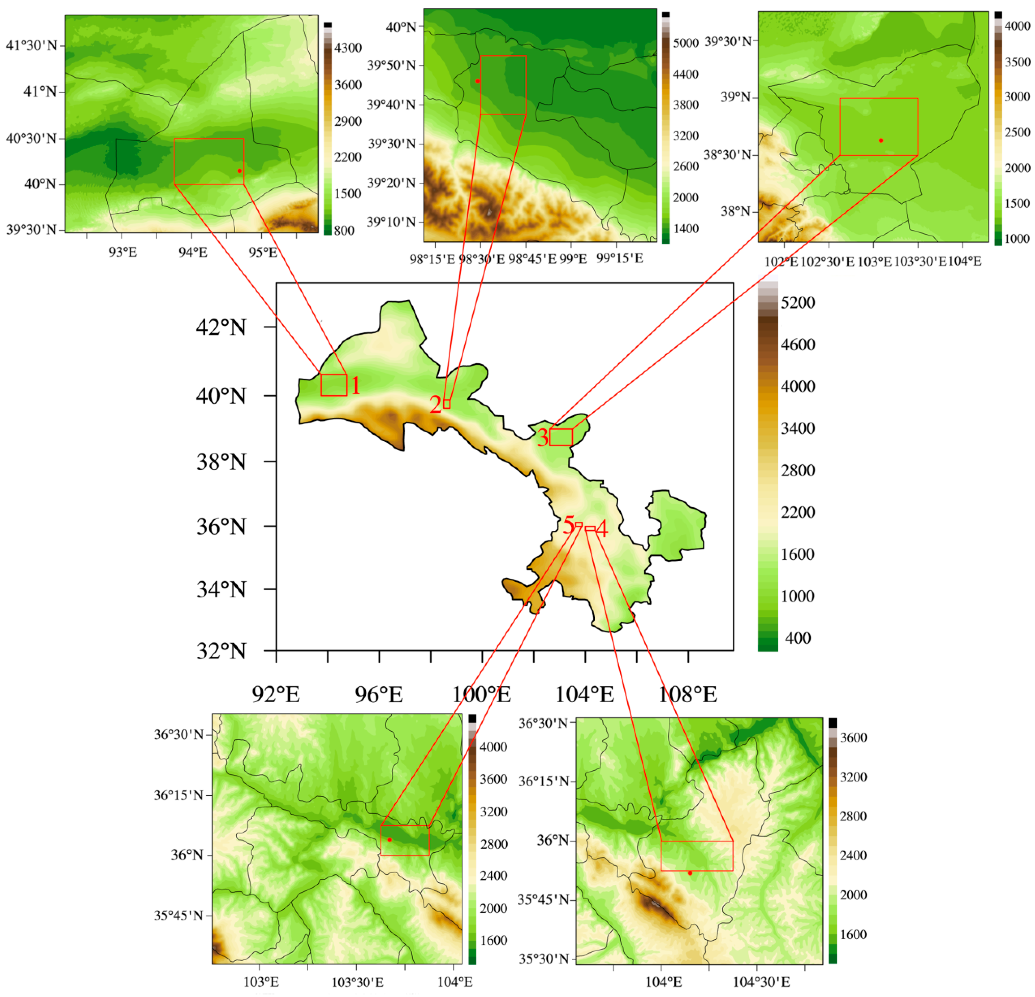
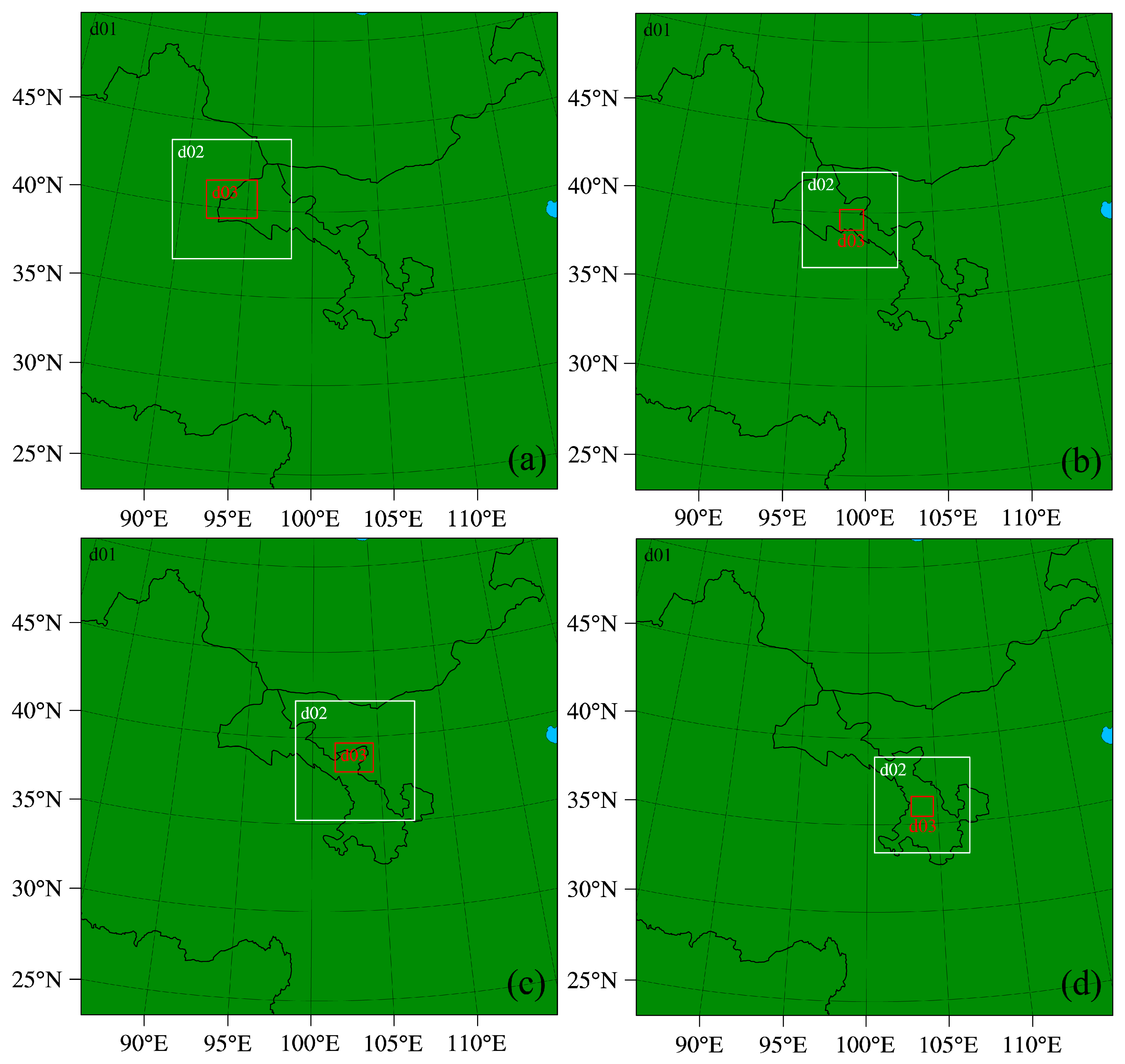
2.3. Scope of Research and Representative Regions

The scope of the paper is from the extreme arid to the semi-arid region in northwest China (Figure 1), including the following representative regions: (1) Dunhuang, with a surface cover that is mainly desert and gobi, is located in the western end of the research area. It is a typical extreme arid area with extremely low vegetation coverage. (2) Jiuquan is located in the midwest of the research area, where the terrain is open and flat, with a surface covering that is mainly desert. It is a severe arid area. (3) Minqin, located in the middle of the research area, consists of three basic landforms, desert, low hill and plain. It belongs to the arid climate zone. (4) Yuzhong and (5) Lanzhou are located in the southeast of the research area. Lanzhou is a typical valley urban city, whereas Yuzhong is a suburb located in the southeast of Lanzhou. These two regions are typical semi-arid climate regions.

2.4. Numerical Model

The WRFv3.8 model adopted in this paper is a new generation of mesoscale weather forecasting models, jointly developed by the National Center for Atmospheric Research (NCAR) and National Centers for Environmental Prediction (NCEP) and other departments, which is widely used in atmospheric science research and forecast. The applicable scale of WRF is from tens of meters to thousands of kilometers, using Arakawa C grid in a horizontal direction. The vertical coordinates use terrain-following static pressure. WRF provides a wealth of radiation, a boundary layer, micro-physical process, land surface process, cumulus convection and other parameterization schemes.

3. Characteristics of Atmospheric Boundary Layer Height in Arid and Semi-Arid Regions

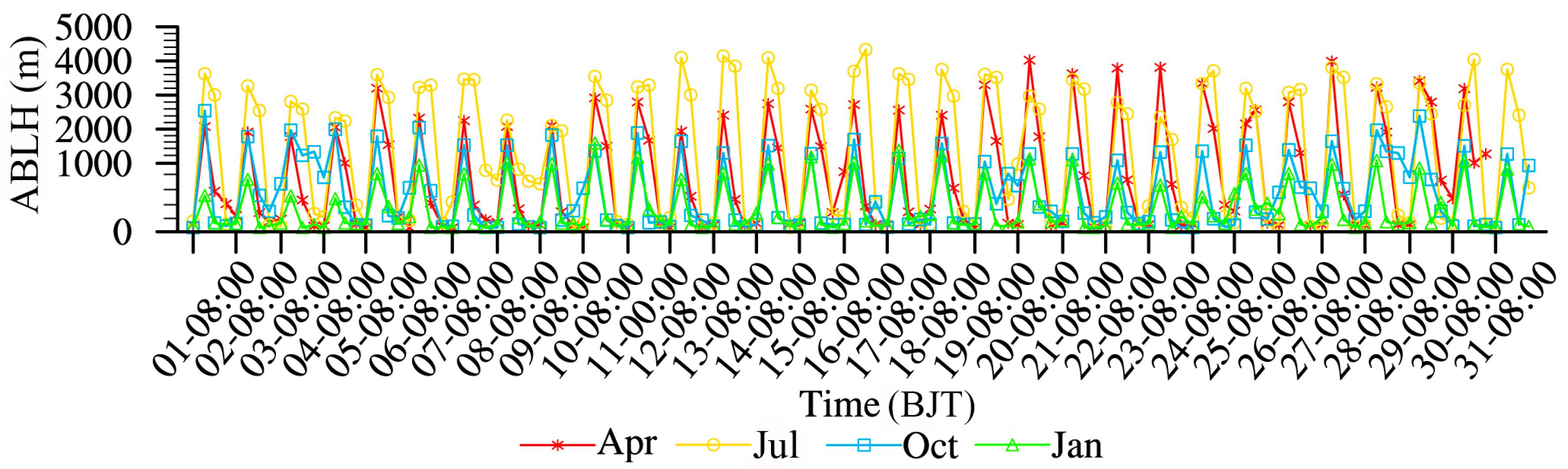
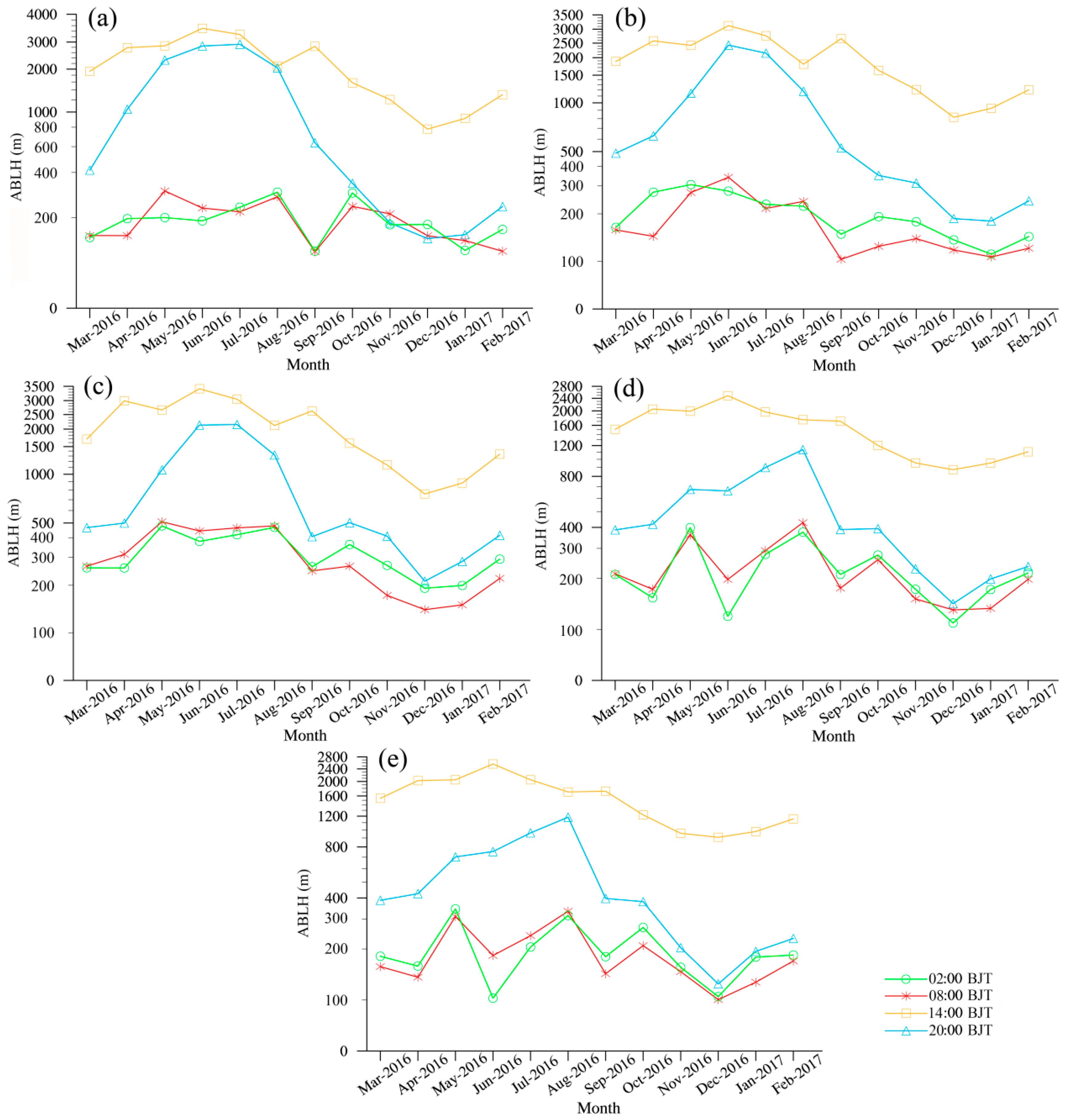
3.1. Monthly Variation of Atmospheric Boundary Layer Height

The heights of the atmospheric boundary layer in the five representative regions (Dunhuang, Jiuquan, Minqin, Lanzhou, and Yuzhong) are calculated by the ERA-Interim reanalysis data from 1 March, 2016, to 28 February, 2017, which have significant characteristics of seasonal distribution (Figure 2). Dunhuang represents the extremely arid area, with a deep-developed boundary height that reaches a peak at 14:00 BJT (Figure 2a), with an annual average of 2088 m, and the average of June is as high as 3505 m, which is the highest in the year, and the lowest in December is 778 m. At 20:00 BJT, the developed boundary layer of Dunhuang reaches the second highest with an annual average height of 1107 m. At the time, the highest height is 2914 m in July and the lowest is 149 m in December. Boundary layer heights over 2000 m were reached in Dunhuang at 06:00 and 20:00 BJT from May to August. Meanwhile, the development of the deep boundary layer lasts at least 6 h in summer. However, the heights reduce below 800 m and the duration shortens in autumn and winter. The height at 08:00 and 02:00 BJT has no significant difference to the annual variation, with average heights of approximately 190 m. This means the atmospheric boundary layer height at night and in the morning is relatively stable with little change, and the maximum value is does not exceed 300 m.
The seasonal average of the boundary layer height in Dunhuang: summer > spring > autumn ≈ winter, with values of 1512, 1042, 662 and 369 m, respectively. From noon to afternoon, in each season, the probability that a deep-developed boundary layer will be developed in the daytime is great. The largest change of the monthly average height in a year is at 20:00 BJT, which is an important time to switch from daytime to nighttime. The change could better reflect variation of convective energy between the months. The height difference between the atmospheric boundary layer at 14:00 and 20:00 BJT is manifested as winter > autumn > spring > summer, which is opposite to the seasonal distribution of the boundary layer height. The boundary layer at 14:00 BJT developed vigorously to a height with a difference of 1967 m between summer and winter. However, at 20:00 BJT the maximum difference between the two seasons is as high as 2421 m. The larger difference at 20:00 BJT may be related to the time of unstable transformation into stable boundary layer for late sunset in summer but early sunset in winter.
Considering the boundary layer height analysis of the extremely arid area in Dunhuang, similar characteristics of the height have been found in the arid areas, Jiuquan (Figure 2b) and Minqin (Figure 2c), and in the semi-arid areas, Yuzhong (Figure 2d) and Lanzhou (Figure 2e). The deep-developed boundary layer appears at 14:00 BJT in all seasons and the largest seasonal change is still at 20:00 BJT. The heights at 08:00 BJT and 02:00 BJT are small as in Dunhuang. The height order in the four representative areas is summer > spring > autumn ≈ winter. However, the deep-developed boundary layer in summer that lasts exceeds 6 h gradually decreases from arid areas to semi-arid areas. As in Dunhuang, the height at 20:00 BJT has the largest changes between the months. The development of the deep-developed boundary layer is postponed from June to August, although the highest atmospheric boundary layer height still appears in June. At 08:00 BJT and 02:00 BJT, the variation characteristics of the boundary layer height in Dunhuang, Jiuquan and Minqin are similar, with high height in spring and summer, and low heights in autumn and winter, but a relatively gentle change. The height variations at the time show more wave style in Yuzhong and Lanzhou, and may be influenced by the local mountainous terrain.
The development of the boundary layer is powered by solar radiation, showing a certain correlation between the boundary layer height and the air temperature (Table 1). The boundary layer heights are all positively correlated with the air temperature, except for at 02:00 BJT in Jiuquan (did not pass the significance test). The largest correlation coefficient appears at 14:00 BJT with an average of 0.718 in the five regions. The correlation coefficient at 20:00 BJT is slightly lower than that at 14:00 BJT, and the average in the five regions is 0.579. However, the correlations between the height and the temperature at both 14:00 and 20:00 BJT in the arid regions (Dunhuang, Jiuquan and Minqin) are higher than those in the semi-arid regions (Yuzhong and Lanzhou). The height of the deep-developed boundary layer is relatively more dependent on the air temperature at 14:00 and 20:00 BJT than at 08:00 and 02:00 BJT when other factors are taken into consideration to influence the boundary layer development.
A more detailed analysis was conducted on the development of the atmospheric boundary layer in April, July, and October 2016 and January 2017 in Dunhuang (Figure 3). The boundary layer height has an obvious daily change cycle. In some cases, the atmospheric boundary layer height in July was below the height in the other months but, on average, it is higher in July. The conclusions have similar characteristics in Jiuquan, Minqin, Yuzhong and Lanzhou (figure omitted). The following section will study the occurrence of the extremely high atmospheric boundary layers in the four seasons.

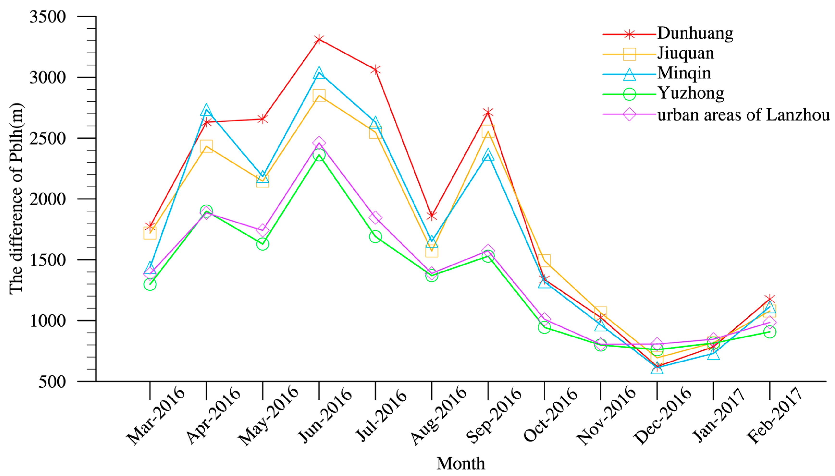
3.2. Deep-Developed Boundary Layer Height in Daytime

Due to the special geographic environment and climate characteristics of northwest China, a relatively deep-developed boundary layer was observed [3]. It generally occurs when the convection development is available in the afternoon. According to the above calculation, the deep-developed boundary layer generally occurs at 14:00 BJT. Thus, the height at 14:00 BJT is divided into five levels and their frequencies are calculated in the four seasons (Table 2). Characteristics of the deep-developed boundary layer that exceeded 2000 m are mainly studied in the five representative areas and the atmospheric boundary layer with a height greater than 4000 m is defined as the extremely high atmospheric boundary layer.
In spring, the most frequent height grade in Dunhuang is 2000–3000 m, accounting for 38%. The second is 1000–2000 m, accounting for 32%. The last is 3000–4000 m, accounting for 24%. The boundary layer height over 4000 m appears six times, but accounts for 29% of the annual total number. The extremely high atmospheric boundary layer occurs once at the end of April and five times in May. In these two months, a deep-developed boundary layer over 2000 m has accounted for 68%. In summer, the boundary layer height of 2000–4000 m has accounted for 73% of the total frequency. The boundary layer heights exceeding 4000 m appeared 13 times, which accounted for 62% of annual appearances, with 10 in June and 3 in July. The frequency of the deep-developed boundary layers in autumn is relatively small and the most frequent height is 1000–2000m. In winter, the height of the atmospheric boundary layer is less than 1000 m.
Minqin is also an important desertification area. The frequency distribution of the boundary layer height at different levels is similar to Dunhuang. The boundary layer exceeding 4000 m mainly appears in summer. Compared to Minqin, Jiuquan is closer to Dunhuang. But Jiuquan vegetation coverage is greater than Dunhuang. Its frequency distribution also differs from Dunhuang. The greatest frequency of the height is between 1000 m and 2000 m, and the second is 2000–3000 m. The extremely high atmospheric boundary layer appeared six times in summer, which is half number in Dunhuang or Minqin. The frequency of the deep-developed boundary layer has been greatly reduced in autumn and winter, with heights just over 3000 m. In the semi-arid region, the frequency distribution of the atmospheric boundary layer heights is similar in the five level grades in Yuzhong and Lanzhou, mainly ranging from 1000 to 2000 m and then 2000 to 3000 m. The height of the extremely atmospheric boundary layer only appears in spring and summer. The height in autumn and winter rarely exceeds 3000 m and the height over 2000 m is less than 6% of the total number. Whether in the arid region or the semi-arid region, the atmospheric boundary layer height exceeding 2000 m is very rare in winter.
In summary, the frequency of the boundary layer height at the five levels in each area has its seasonal distribution characteristics. The deep-developed boundary layer height mainly occurs in summer, followed by late spring. The highest atmospheric boundary layer heights that exceed 4000 m, even 5000 m in Minqin, are mainly distributed in June. The frequency, duration, and maximum height of the boundary layer show obvious differences in the arid region and the semi-arid region. The spatial distribution of the deep-developed boundary layer will be further discussed in the following section.

4. Spatial Distribution and Weather Influence

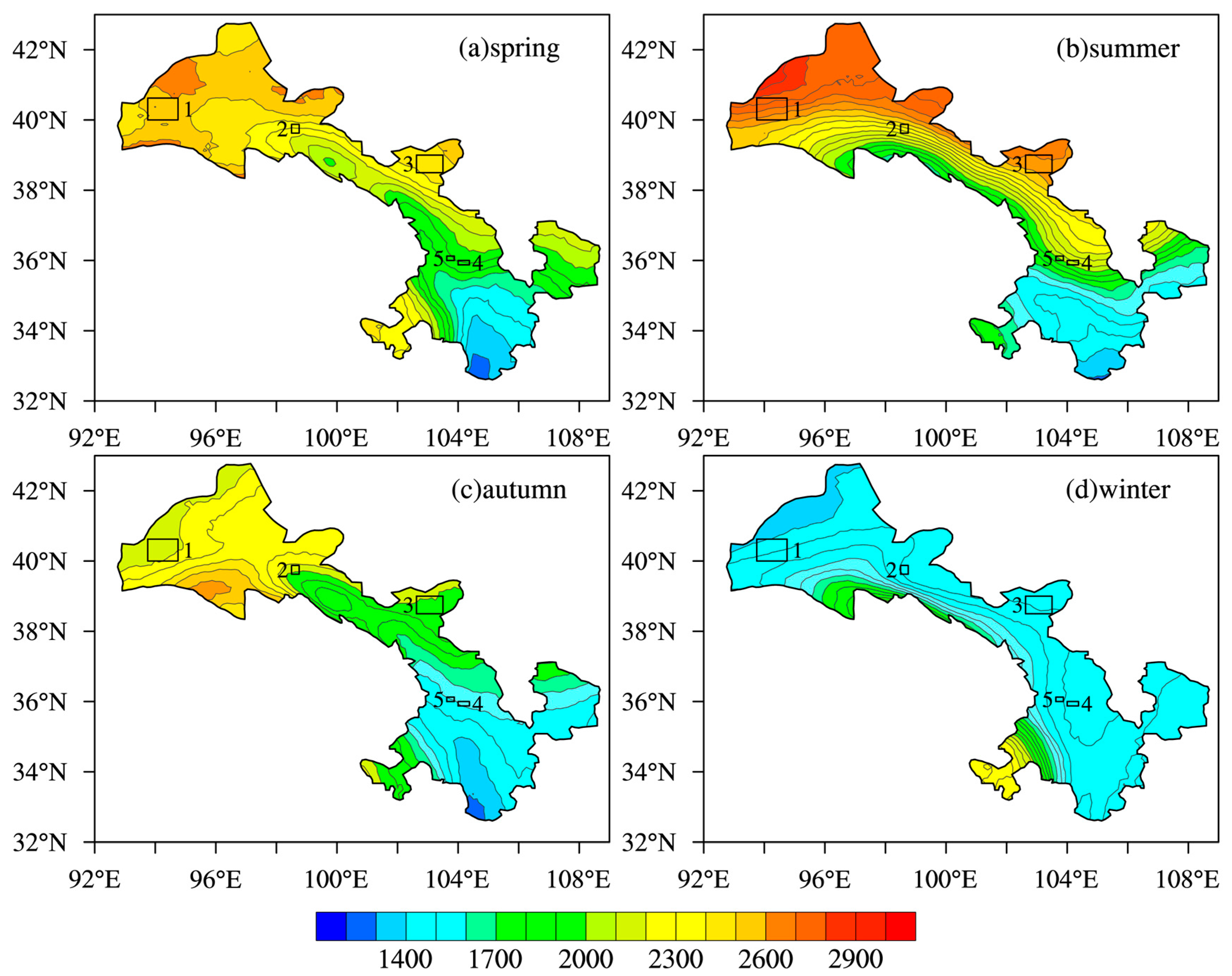
4.1. Spatial Distribution of Atmospheric Boundary Layer Height

The previous section showed the variation characteristics of the atmospheric boundary layer height in five representative regions which do not fully stand for arid and semi-arid regions in northwest China. The spatial distribution of the deep-developed boundary layer height was probed and will be discussed to locate the maximum and minimum height centers. The spatial distribution of the height at 14:00 BJT in four seasons was presented in Figure 4 with the five representative areas in Gansu province, which range from arid regions to semi-arid regions in northwest China. The numbers 1–5 in the figure represent the areas of Dunhuang, Jiuquan, Minqin, Yuzhong and Lanzhou. Consistent with the results from the above analysis, the deep-developed height of the atmospheric boundary layer is, on the whole, highest in summer, followed by spring, autumn and winter. The development height of the boundary layer decreases from the north to the south and from the west to the east. The maximum value center appears in the vicinity of Dunhuang (position 1 in Figure 4), while the minimum value appears in the south (to the south of position 1 in Figure 4).
It is worth noting that the atmospheric boundary layer height near position 3 is also relatively high. Particularly in spring and summer, the convective layer development is as strong as the atmospheric boundary layer in the extremely arid area, Dunhuang. However, in autumn and winter, the boundary layer height is similar to that in the semi-arid region. Another relatively high atmospheric boundary layer appears to the southwest of position 4, though the location is outside of the arid area. It is higher than in other places, especially in winter. It is located in the Qinghai–Tibet Plateau, where atmospheric boundary layer shows special characteristics.
In detail, the spatial distribution of the atmospheric boundary layer four times per day depicts that the highest and second-highest boundary layer developed at 14:00 and 20:00 BJT, respectively, in summer (Figure 5). The high value centers are found near Dunhuang. To the north of positions 1, 2 and 3 are the areas in which the boundary layer heights are relatively high. The average difference of the boundary layer heights between Dunhuang and Minqin is 102 m at 14:00 BJT, whereas the difference is 300 m between Minqin and Jiuquan and 457 m between Jiuquan and Lanzhou. The gradient of the boundary layer height gradually increases from arid area to semi-arid area. At 20:00 BJT, the arid area still maintained a higher atmospheric boundary layer with little difference in distribution at 14:00 BJT, but a larger decreasing amplitude of the height appears in the semi-arid area. This indicates that the deep-developed boundary layer lasts longer in the arid area than in the semi-arid area, which is consistent with the analysis results of the representative sites and has universal characteristics. Remarkably, the atmospheric boundary layer height at 08:00 BJT and 02:00 BJT in Minqin (position 3) is relatively higher than in the whole region, which may be related to its aridification. The atmospheric boundary layer height at these two times reflects the aridification of the region better. In addition, the spatial distribution characteristics of the boundary layer height at all times in spring and autumn is similar to that in summer, whereas there is little change in the spatial distribution between the four times in winter (figure omitted).
In summary, the high-value center of the study field appears in the northwest near Dunhuang, and the low-value center is located in the southernmost regions. Minqin is another important high-value center with the developed boundary layer, which can be distinctly reflected at 08:00 BJT and 02:00 BJT.

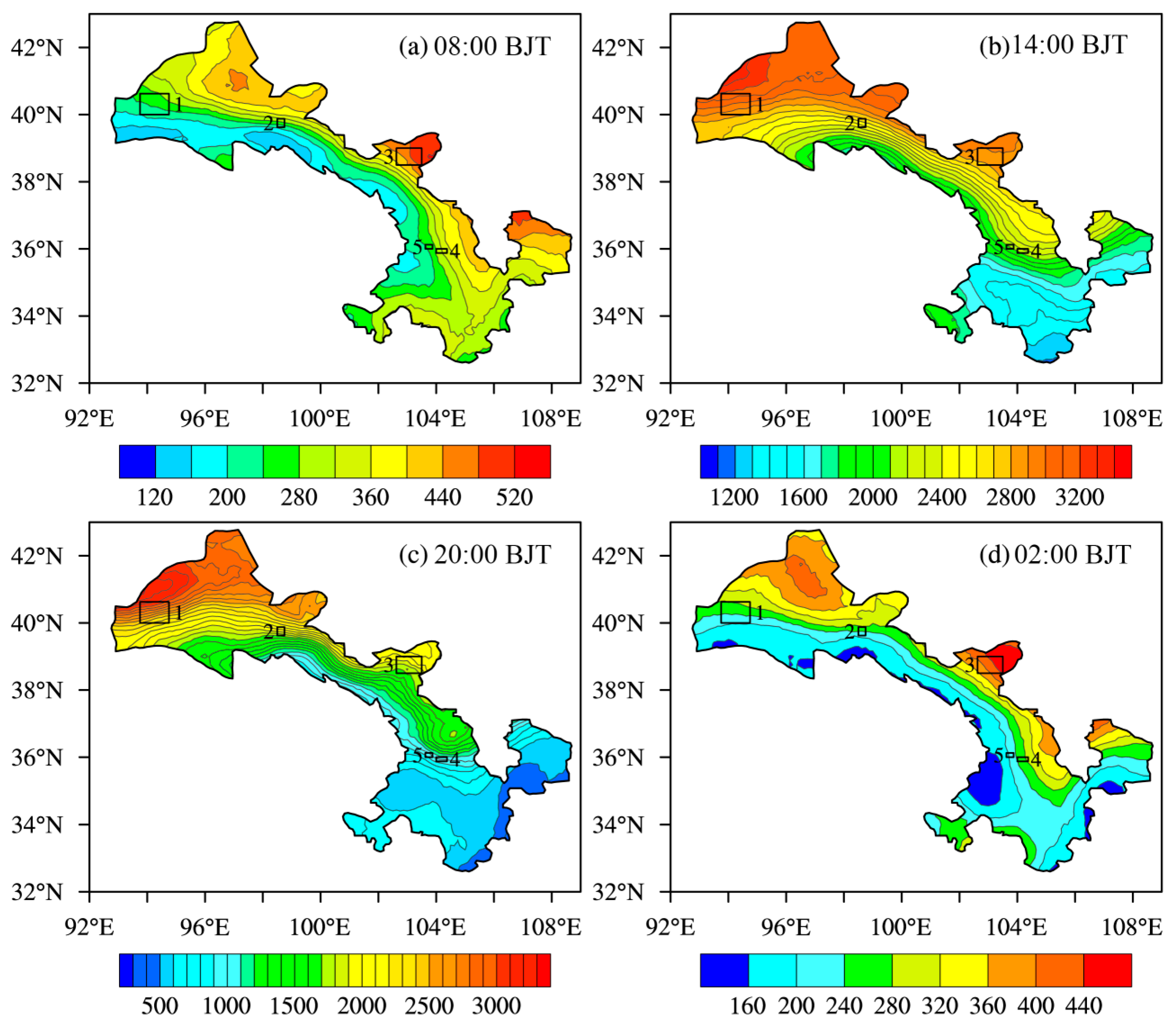
4.2. Weather Influence on Atmospheric Boundary Layer Development

The difference between the maximum and minimum values of the boundary layer height (the mean value of the four times) is used to characterize the change in amplitude of the atmospheric boundary layer development. Figure 6 shows that the change in the development of the boundary layer varies significantly by region and month. The largest change in the atmospheric boundary layer height is found in Dunhuang from May to September, followed by Jiuquan and Minqin. The smallest change in the year is found in Yuzhong and Lanzhou, except December and January. This means there is a great difference in the height between daytime and nighttime in the arid area, and the difference gradually decreases from the arid area to the semi-arid area. The difference in height between daytime and nighttime basically shows three peaks in a year, in April, June and September. The maximum appeared in June, reaching 3311 m in Dunhuang, 2849 m in Jiuquan and 3038 m in Minqin, 2362 m and 2460 m in Yuzhong and Lanzhou, respectively. There is a relatively small gap in August, especially in Dunhuang, Jiuquan, and Minqin. The weather influenced the large drop from July to August (Table 3). The number of precipitation days, cloudy days and overcast days is larger in August than in the other months in Dunhuang, Jiuquan and Minqin. Furthermore, the monthly average of the total cloud amount is also statistically higher in August than in the other months. Days on which the cloud proportion is 0–10%, 10–30%, 30–70% 70–100% are defined as sunny, partly cloudy, cloudy and overcast days, respectively. Generally, the height of the atmospheric boundary layer in cloudy and overcast days is less than in sunny days [29]. Precipitation also inhibits the boundary layer development [30], resulting in small differences between the maximum and minimum height. The development of the boundary layer in the arid area is weakened in winter, and the difference between the maximum and minimum values in December and January is lower in arid areas than in semi-arid areas. Thus, the height of the atmospheric boundary layer is more stable during a whole day in winter. Except for April, the difference is greater in Lanzhou than in Yuzhong. Though the two areas are both located in the semi-arid region and the distance between them is small, Lanzhou is an urban area and Yuzhong is a suburb. The change in amplitude of the atmospheric boundary layer height in a day is greater in Lanzhou due to the urban heat island effect [31,32].

5. Numerical Simulation on Deep-Developed Boundary Layer Height

The radiosonde sounding data at observation sites have low vertical resolution and are observed only twice a day (08:00 and 20:00 BJT), providing less information to describe vertical changes about the atmospheric boundary layer. Although the reanalysis data combined with radiosonde observation data can describe and calculate the height of the atmospheric boundary layer well, only four times every day (08:00, 14:00, 20:00 and 02:00 BJT) are used to analyze the atmospheric boundary. Vertical meteorological elements variation of the atmospheric boundary layer height is still difficult to analyze. Numerical simulation provides a possibility for studying the detailed meteorological process of atmospheric boundary layer development, but the selection of the model parameterization scheme has a direct influence on the boundary layer height simulation results. In the following, the WRF model is used to simulate the deep-developed boundary layer and discuss the influence of different parameterization schemes on the numerical simulation.

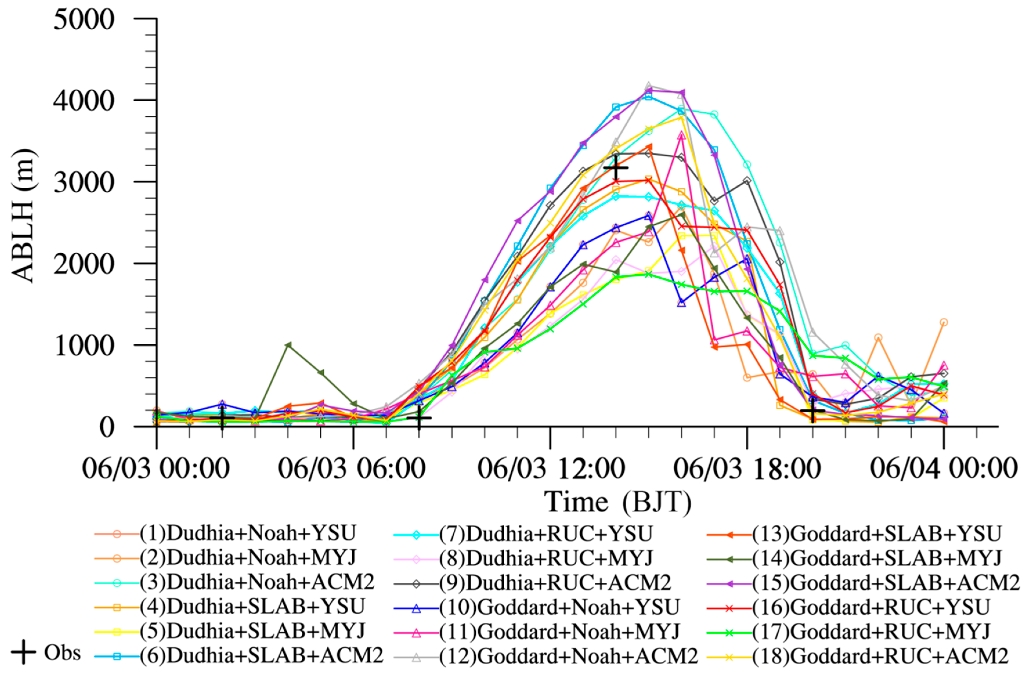
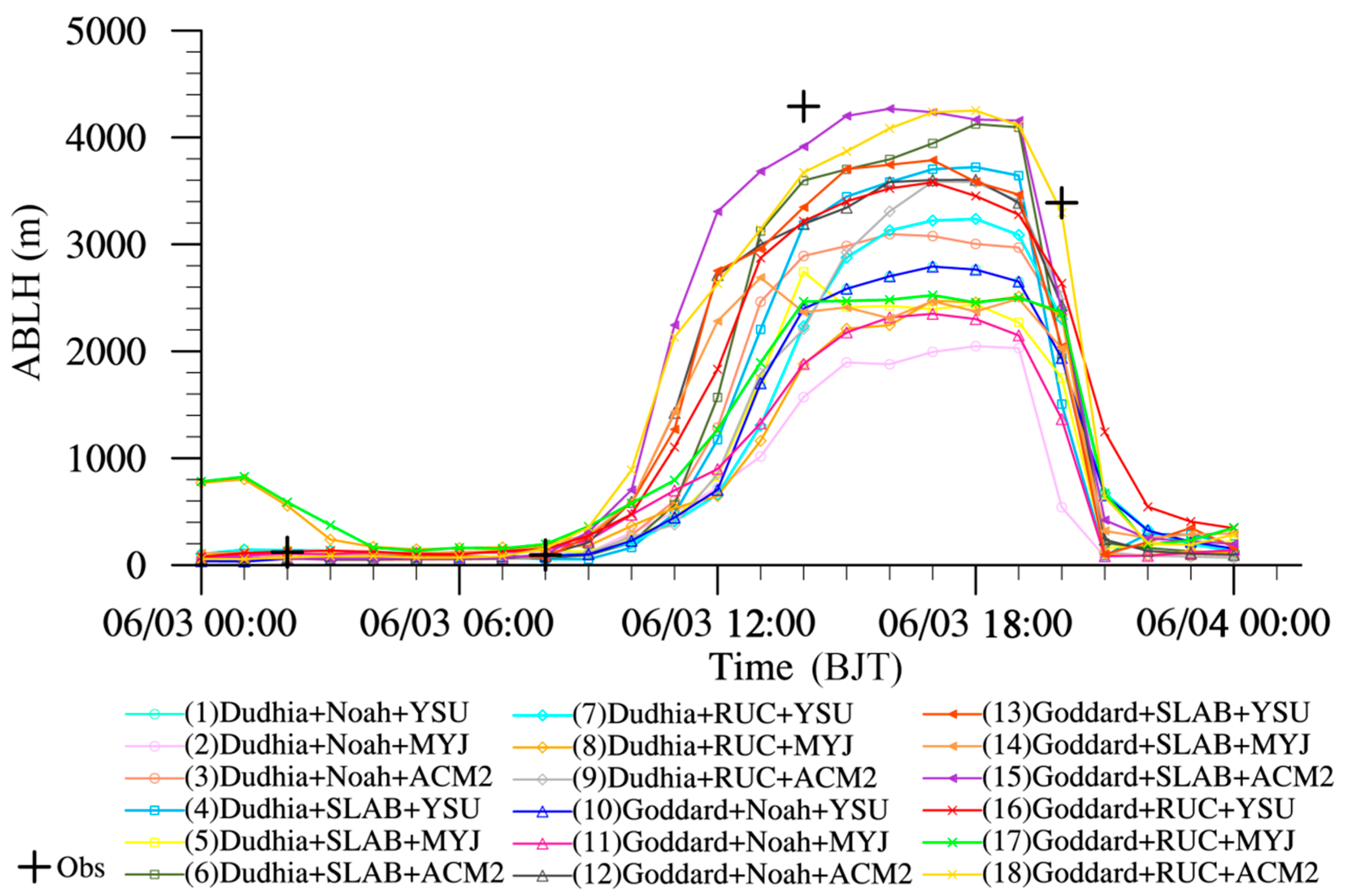
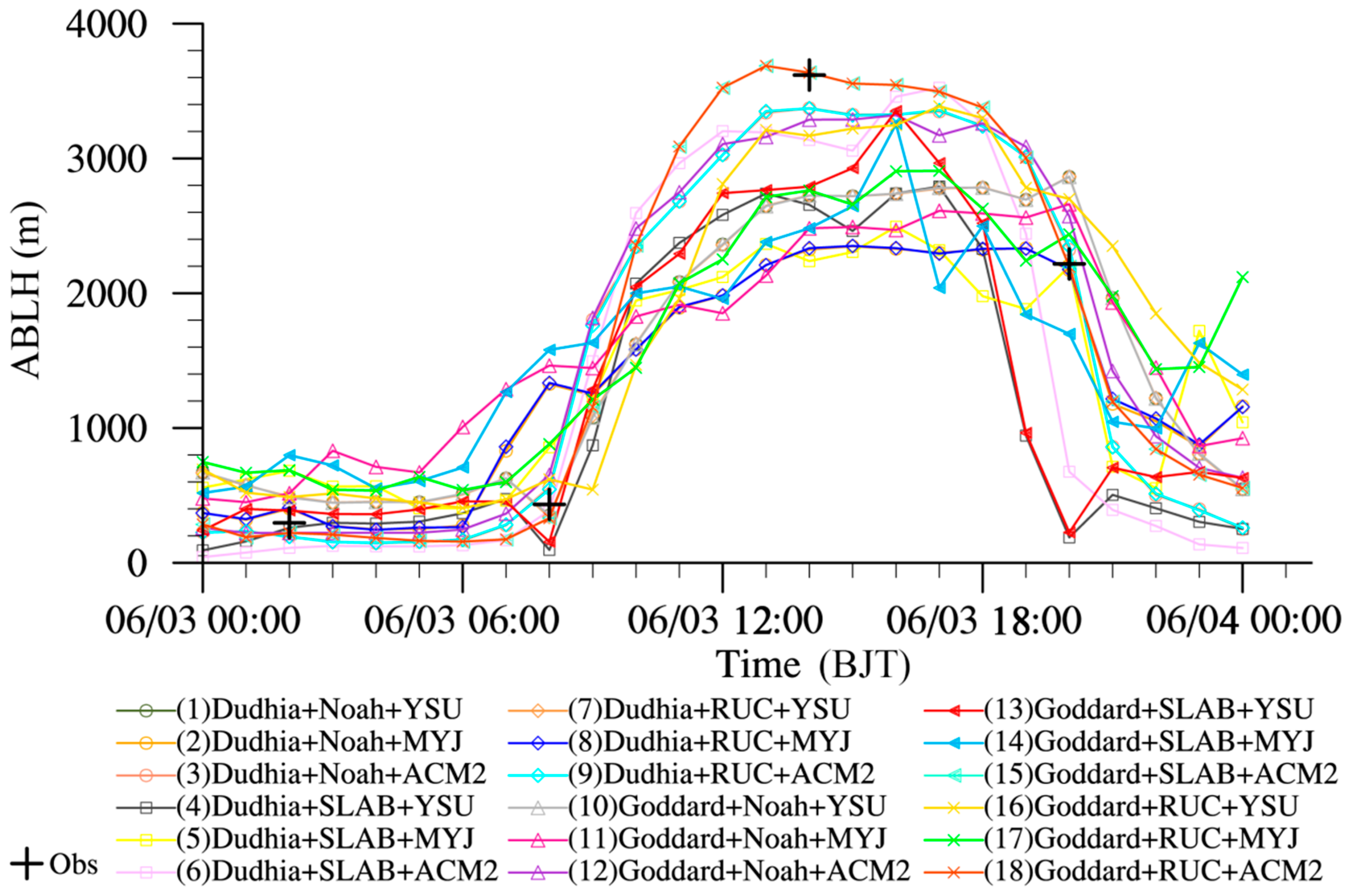
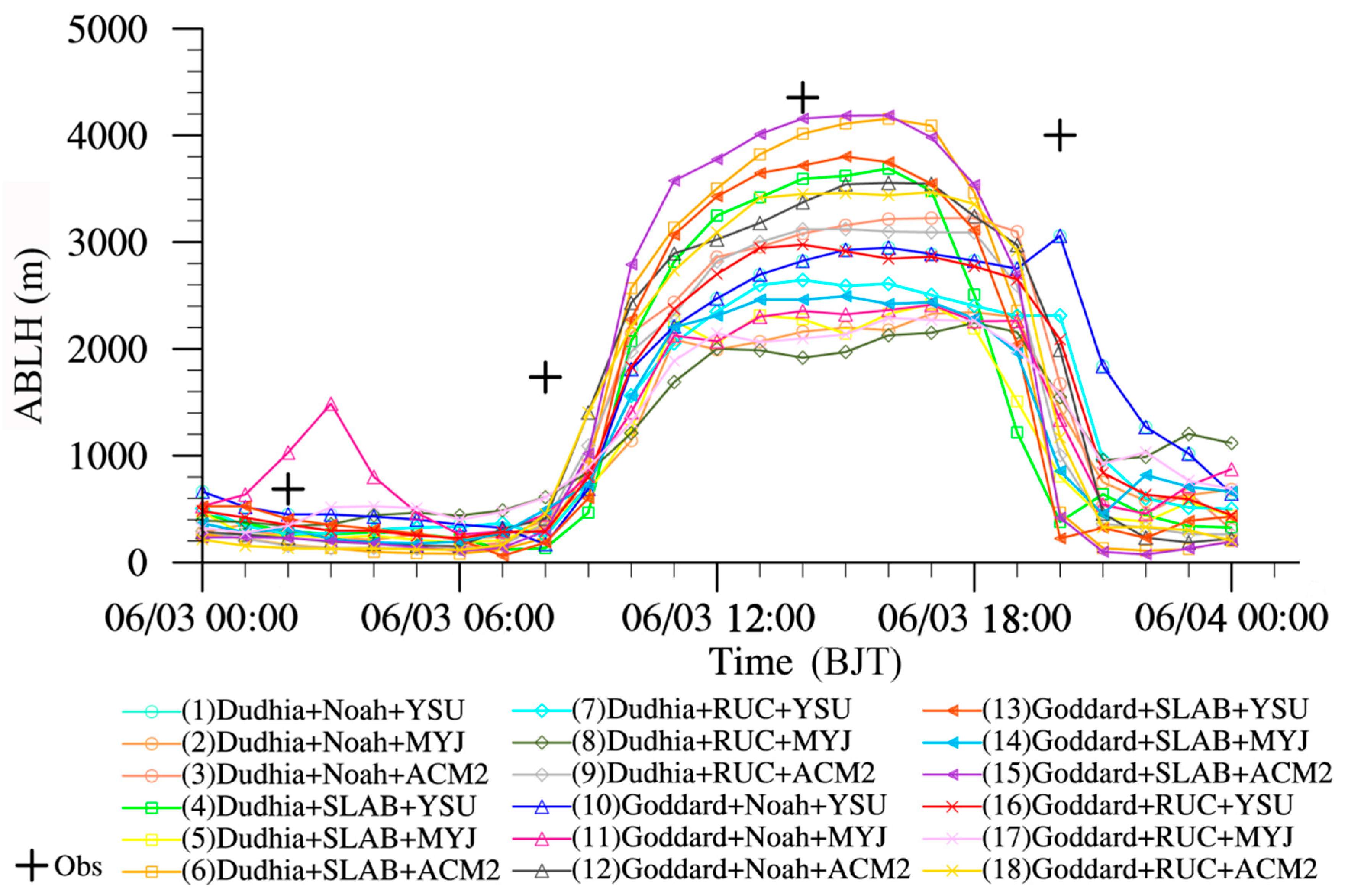
5.1. Experimental Design

The four simulation areas of the numerical simulation designed involve the five representative regions above (Figure 7). All are triple-nested grids with a horizontal resolution of 25, 5, and 1 km, with a common center point (100.5° E, 7.75° N) and 40 layers in the vertical direction. The top pressure is 5 hPa, using 1° × 1° FNL global reanalysis data provided by NECP/NCAR as the initial condition and the boundary condition. The main parameterization schemes are the WSM3 (WRF Single-Moment 3-class) microphysical scheme, RRTM (Rapid Radiative Transfer Model) longwave radiation scheme, and the Kain–Fritsch (new Eta) cumulus parameterization scheme; the third grid has no cumulus convection due to its high resolution (1 km). The combinations of a shortwave radiation scheme, land surface scheme, atmospheric boundary layer scheme and surface layer scheme are shown in Table 4.

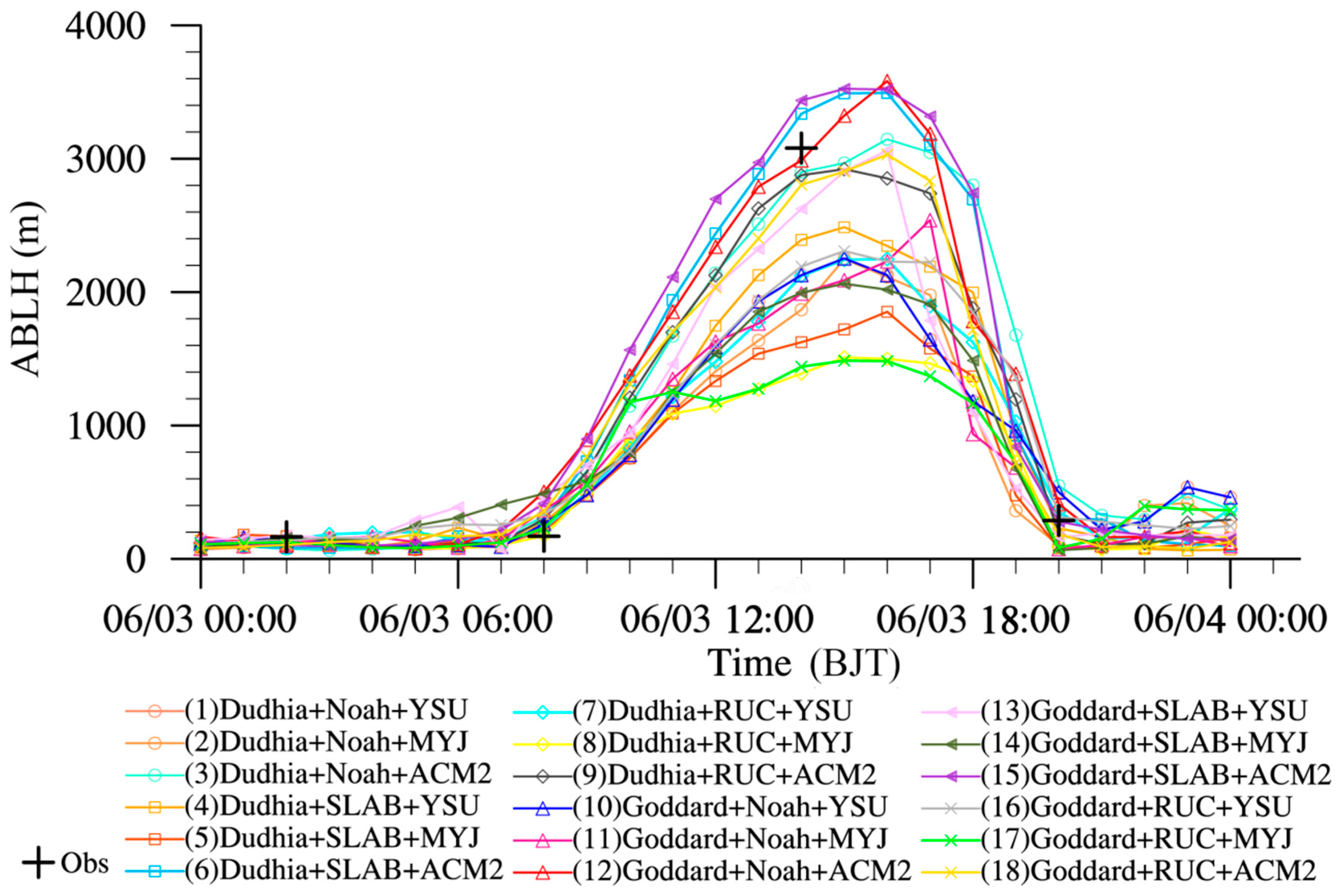
5.2. Simulation Results

Solar radiation provides energy for the development of the atmospheric boundary layer, whereas the solar radiation reaching the ground is related to the shortwave radiation schemes. The energy provided by the surface absorption and reflection for atmospheric deep convective development is directly affected by the land surface parameterization schemes. The boundary layer process is determined by the atmospheric boundary layer parameterization schemes. Therefore, this paper analyzes the influence of the combination of shortwave radiation schemes, land surface schemes, and atmospheric boundary layer schemes on atmospheric boundary layer simulation. Figure 8 shows the observed boundary layer height calculated by the bulk Ri in Dunhuang and the variation of the boundary layer height using the WRF with the different combinations of parameterization schemes. The numerical model can simulate the diurnal variation trend of the boundary layer height in Dunhuang. At 10:00 BJT on 3 June, the boundary layer height began to rise gradually with the increase of solar radiation arriving the ground. From 14:00 to 19:00 BJT, the boundary layer developed to a higher height and persevered several hours, then dropped rapidly. At night, except for combinations 8 and 17 with higher results, the difference is small between the simulation results of the other scheme combinations and the observational results. However, during the daytime, the convective develops strongly, the simulation results of each parameterization scheme combination are low. Minimum bias of the simulation results was captured in combination 15, 376 m lower than the observed result, followed by combinations 18 and 6, 618 and 695 m, respectively. The remaining combinations have a bias of exceeding 1000 m. In the simulation of the Dunhuang deep-developed boundary layer, combination 15 (Goddrad+SLAB+ACM2) is relatively accurate.
Like Dunhuang, the numerical simulation results of Jiuquan can also capture the evolution of the atmospheric boundary layer (Figure 9). The biases of the various combinations of parameterization schemes and observation during the night are smaller than those in the deep-developed boundary layer during the daytime, and the difference between different parameterization schemes is more evident during the daytime. The best combination of simulation effects at 14:00 BJT is still combinations 15 and 18, and other combinations are smaller than the observations. The bias of combination 5 is up to 1381 m, which cannot simulate the height of the deep-developed boundary layer. Minqin is a sever arid area with a high boundary layer height at night. In addition, the simulation results of combination 11 at 02:00 BJT on 3 June are higher than the observed values, and the combination results of each numerical simulation parameterization scheme are lower than the observed values (Figure 10). The best simulation result for the deep-developed boundary layer is combination 15. The simulated value is 197 m lower than the observed value, followed by combination 6. The bias of the other combinations exceeded 600 m. At 20:00 BJT on 3 June, the boundary layer height of Minqin remains at 4000 m. Except for combination 1, at that time, the value increased, the biases of rest combinations exceeded 2000 m, and no deep-developed boundary layer was simulated. Overall, in extreme arid and arid areas, the atmospheric boundary layer had a high level of development. The best combination of parameterization schemes for deep-developed boundary layer numerical simulation is combination 15 (GODDRAD+SLAB+ACM2), but the numerical simulation results are generally lower than those observed.
Unlike for the arid regions, numerical simulations of the atmospheric boundary layer height in the Yuzhong and Lanzhou areas of the semi-arid region (Figure 11 and Figure 12) show that some of the combinations are higher than the observations, and some are lower than the observations. Minimum bias of the Yuzhong deep-developed boundary layer height simulation was for combination 12 (−92 m), followed by combination 3 (−179 m) and combination 9 (−203 m), and the combination 15 simulation results are higher. The minimum simulation bias of the deep-developed boundary layer height in Lanzhou is the combination 13 (+24 m), followed by the combination 3 (+128 m), the combination 16 (−169 m) and the combination 9 (+170 m). Secondly, numerical simulations captured the development characteristics of the atmospheric boundary layer in the semi-arid regions. Compared to the arid area, the deep-developed boundary layer in Yuzhong and Lanzhou remained relatively short (about 3–4 h). However, in the simulation, the majority of the results of the combination of the schemes still do not exceed the observed deep-developed boundary layer height. In conclusion, the deep-developed boundary layer in the semi-arid region, the numerical model parameterization scheme combination 12 (Goddard+Noah+ACM2), combination 3 (Dudhia+Noah+ACM2) and combination 13 (Goddard+SLAB+YSU) have a good effect.
In summary, the WRF model can simulate the diurnal variation of the atmospheric boundary layer height. The duration of the deep-developed boundary layer in summer is not the same. The deep-developed boundary layer of Dunhuang, Jiuquan and Minqin is maintained for approximately 6–7 h, whereas in Yuzhong and Lanzhou, it is maintained for approximately 3–4 h. The simulation effect of different combinations of parameterization schemes is not the same in different regions. The simulation results for Dunhuang, Jiuquan, and Minqin are better with combination 15, and the simulation results are all slightly lower. The simulation results in Yuzhong and Lanzhou are better with combination 3, and the results are high.
Three physical schemes selected to the simulation show obvious differences in different combinations. With fixing two parameterization schemes, the other one parameterization scheme was analyzed in the simulation results (Table 5). For example, for the fixed shortwave radiation scheme and land surface scheme, the average value of the bias of the simulation results of the third atmospheric boundary layer schemes in three options was calculated. The results show that the maximal average value of the bias in five regions is the atmospheric boundary layer scheme; the choice of the atmospheric boundary layer scheme has the greatest impact on the simulation results. Except for Jiuquan, the minimum average value of the bias is the shortwave radiation scheme.
No matter which shortwave radiation scheme or land surface process scheme is selected, the simulation results of the three atmospheric boundary layer schemes show that the ACM2 scheme results are the highest in the five regions of the daytime atmospheric boundary layer, followed by the YSU scheme and the MYJ scheme. The three atmospheric boundary layer schemes have different methods to determine the boundary layer height, which is an important reason for the difference in the simulation results. The YSU scheme [34] uses the Richardson number to calculate the boundary layer height:
R i b = g h ( θ v ( h ) θ s ) θ v a U ( h ) 2
where θs is the appropriate temperature near the surface, θva is the virtual potential temperature at the lowest model level, U(h) is the horizontal wind speed at h, and θv(h) is the virtual potential temperature at h. When Rib = Ricri (critical bulk Richardson number), the corresponding h is the boundary layer height, Ricri = 0.25 in stable conditions and Ricri = 0 in unstable conditions. The temperature near the surface is defined as θs = θva + θT,
θ T = b ( w θ v ¯ ) 0 w s
where θT is the virtual temperature excess near the surface and ws is the mixed-layer velocity scale. The virtual heat flux from the surface is ( w θ v ¯ ) 0 and the proportionality factor b is set as 7.8. First, h is estimated by the bulk Richardson number without considering the thermal excess θT (θs = θva). This estimated h is utilized to compute ws and θT. Using ws and θT, h is enhanced. Ricri = 0 eliminates the excessive boundary layer height calculated when there is a certain large wind speed. The ACM2 scheme [35] also uses the Richardson number to compute the boundary layer height. For stable conditions:
R i = g h ( θ v ( h ) θ v ( z 1 ) ) θ ¯ v U ( h ) 2
where θv(h) is the virtual potential temperature, z1 is the height of the lowest model level, and θ ¯ v is the average virtual potential temperature between the layer 1 and h. For unstable conditions, first the top of the convectively unstable layer (zmix) is found as the height at which
θ v ( z m i x ) = θ s = θ v ( z 1 ) + b ( w θ v ¯ ) 0 w m
where b = 8.5, θv(z1) is the potential temperature at the lowest model level, ( w θ v ¯ ) 0 is the sensible heat fluxes from the surface, wm is the scale of convective velocity. Second, calculation of the boundary layer height is based on the Richardson number:
R i b = g ( θ v ( h ) θ s ) ( h z m i x ) θ ¯ v ( U ( h ) U ( z m i x ) ) 2
where θv is the potential temperature, θs is the potential temperature at the surface, and U is the horizontal wind speed. The corresponding h is the boundary layer height when Rib = Ricri = 0.25. Due to the different value of Ricri in the unstable layer between the YSU scheme and the ACM2 scheme, the result of the ACM2 scheme is slightly higher than the YSU scheme. The MYJ scheme [36] defines the height at which the turbulence intensity drops to a critical value of 0.001 m2s−2 as the boundary layer height. The MYJ scheme is more suitable for stabilizing the boundary layer and the weak and unstable boundary layer, so the simulation effect on the deep convective boundary layer is poor.
Comparing the three land surface schemes, the simulation results of Dunhuang SLAB and RUC are higher than Noah. The simulation results of the three kinds of land surface schemes in Jiuquan are not very different. The simulation result of SLAB is higher than that of RUC and Noah in Minqin. The simulation results in Yuzhong are SLAB ≥ Noah ≥ RUC, and they have their own advantages in Lanzhou. The SLAB scheme [37] (5-layer thermal diffusion scheme) is based on the MM5 (Mesoscale model) 5-layer soil temperature model. The energy calculation of the SLAB scheme includes radiation, sensible heat and latent heat flux; the calculations focus on describing changes in surface temperature at high frequency and short time scales. However, the SLAB scheme did not consider the vegetation evapotranspiration and runoff process, having only considered the evaporation of bare soil. The Noah program [38] can be forecasted by 4-layer soil temperature and moisture. The vegetation and soil types and the monthly vegetation index were considered in the process of evaporation and transpiration. The Noah scheme improves urban coverage and takes into account the surface radiation coefficient. The RUC scheme [39,40] contains six layers of soil and two layers of snow cover processing. The temperature and density change of frozen soil and snow, vegetation influence and canopy transpiration were considered. The plant types in the same grid remain the same. The effects of transpiration on water are considered by evapotranspiration parameters related to soil type. Among the three parameterization schemes, the SLAB scheme is simple, Noah and RUC are more complex, and the RUC scheme is more complex than the Noah scheme for considering vegetation, snow, and soil. The development of the atmospheric boundary layer is closely related to the surface-air temperature difference and the near-surface sensible heat flux [41], and different treatment of the soil moisture in each land surface scheme, which makes heat flux and the surface temperature different from each others [42]. The sensible heat flux is directly used in the calculation of the atmospheric boundary layer height and has a greater influence on the simulation results of the atmospheric boundary layer height. The SLAB program only considers the heat transfer of the soil. The soil moisture has two constant values which shows only in winter and summer. The result is sensitive to the soil temperature, and the simulated boundary layer height is often large. Noah and RUC use Richardson number to calculate the soil moisture in each layer. The simulated soil moisture is higher than that of SLAB. The arid regions of Dunhuang, Jiuquan and Minqin are deserted and desert based, with sparse vegetation, dry air, and low soil moisture in summer. Therefore, the SLAB scheme, without consideration of vegetation evapotranspiration and soil moisture, will get a higher atmospheric boundary layer height. The semi-arid area is relatively rich in vegetation on the underlying surface of Yuzhong and Lanzhou and features the underlying surface of the city. The Noah scheme is more suitable for simulating the development of the atmospheric boundary layer in the region. Although shortwave radiation schemes have a little influence on the simulation results, the simulation results of Dudhia scheme in the most combinations in Dunhuang, Jiuquan and Minqin, namely in arid areas, especially in the afternoon, are slightly lower than those of the Goddard Scheme. The simulation results of two shortwave radiation schemes for Yuzhong and Lanzhou, namely in the semi-arid area, are basically the same. The Dudhia scheme [43,44] simply considers clear-sky scattering and water vapor absorption. Vapor absorption under clear sky conditions is calculated as a function of the water vapor, considering approximate Rayleigh scattering and aerosol scattering. The Goddard scheme [45] calculated the solar radiation flux due to the absorption and scattering effects of water vapor, O3, CO2, O2, cloud and aerosols. The radiation reaching the ground directly determines the near-surface energy conditions and the release of surface sensible heat and latent heat [46]. The absorbed energy at the surface is not only dependent on solar radiation transmission, but also closely related to CO2, water vapor, and O3 in the atmosphere. Strong absorption of radiation by CO2 and O3 is also an important source of atmospheric energy and power [47]. The Goddard scheme deals more with CO2 than the Dudhia scheme. The flux reduction caused by CO2 can be obtained from the pre-calculated table, which also considers O3 which is not considered in the Dudhia scheme. This makes the energy obtained from the low-level atmosphere simulated by the Dudhia scheme slightly smaller than that of the Goddard scheme. The simulated boundary layer height is also slightly lower than that of the Goddrad scheme.

6. Results and Discussion

This comparative study focuses on the atmospheric boundary layer height and its characteristics in the arid region (Dunhuang, Jiuquan, Minqin) and the semi-arid region (Yuzhong and Lanzhou) in northwest China. The following conclusions have been drawn:
(1) The boundary layer height in the five representative areas has obvious characteristics of inter-monthly variation. Summer (June) is the season (month) when the atmospheric boundary layer height is the highest compared to the others. During the daytime, the atmospheric boundary layer height in the arid region is much higher and the duration of the deep-developed atmospheric boundary layer is longer than that in the semi-arid region. From May to August, the atmospheric boundary layer has an average height over 2000 m in Dunhuang (the extremely arid region) with a duration exceeding 6 h. But the duration exceeding 6 h only occurs from June to July in Jiuquan and Minqin. The height analysis four times per day showed that the boundary layer developed to the highest level at 14:00 BJT both in the arid and semi-arid regions. There is a large difference at 20:00 BJT between arid and semi-arid regions, but the difference is small at night. The extremely high atmospheric boundary layer defined in the paper is also mainly found in the arid region such as Dunhuang and Minqin, where the highest height even exceeds 5000 m in summer.
(2) The atmospheric boundary layer height decreases from the north to the south and from the west to the east in the research field. The highest height of the atmospheric boundary layer is found in summer and the second-highest in spring and autumn. The highest atmospheric boundary layer generally appears near Dunhuang and the second-highest appears in Minqin. There is a great difference in height between daytime and the nighttime in the arid region but the difference gradually decreases from the arid region to the semi-arid region. The atmospheric boundary layer height is reduced to a small value after August and it may be related to the solar radiation.
(3) The WRF simulation of the atmospheric boundary layer height shows obviously different results in different combinations of parameterization schemes. The deep-developed boundary layer height simulated in the arid area is less overall than the observed value but the simulated heights in the semi-arid area have both higher and lower values compared to the observed value. In the combinations of shortwave radiation, land surface processes and boundary layer parameterization schemes, the most suitable combination in Dunhuang and Minqin is Goddard+SLAB+ACM2, and in Jiuquan is Goddard+SLAB+ACM. In the semi-arid region, Dudhia+Noah+ACM is suitable for the simulation in both Yuzhong and Lanzhou.
(4) The effects of the three parameterization schemes are different from each other on the numerical simulation results. The effects also slightly change with the regions. The influence of the three schemes on the deep boundary layer in the research field presents an important order as boundary layer scheme > land surface process > short wave radiation scheme, whereas there is little difference in Jiuquan. The difference between the boundary layer parameterization schemes is as high as approximately 1200 m. Of the three atmospheric boundary layer schemes, the ACM2 scheme is the best scheme in all five areas, followed by YSU and MYJ. The reason for this is related to the different methods to determine the boundary layer height in the three schemes. Of the land surface process parameterization schemes, the highest boundary layer is simulated by the SLAB scheme because the scheme is based on the 5-layer soil temperature thermal diffusion model and its results are sensitive to soil temperature. Although the shortwave radiation schemes have little impact on the simulation results, the simulation by the Dudhia scheme shows slightly lower height than that by the Goddard scheme. The schemes have different treatments for the transmission and absorption of solar radiation.

7. Conclusions

In summary, the simulation result of the atmospheric boundary layer height is directly related to arid and semi-arid regions. On the other hand, the climate change is fed back by the atmospheric boundary layer development. To obtain a more accurate numerical simulation, the characteristics, time and area of research should be taken into consideration in parameterization scheme settings.

Author Contributions

Conceptualization, M.M.; methodology, M.M., Z.T., F.D.; software, Z.T.; validation, F.D., Y.C. and Y.Y.; formal analysis, M.M.; investigation, M.M.; resources, F.D.; data curation, Z.T.; writing—original draft preparation, Z.T.; writing—review and editing, M.M., Y.C., Y.Y.; visualization, Z.T.; supervision, M.M.; project administration, M.M.; funding acquisition, F.D.

Funding

This research was funded by Drought Meteorological Science Research Fund Project, grant number IAM201603; Gansu Province natural sciences foundation, grant number 18JR3RA278; National Key R&D Program of China, grant number 2017YFC1501805.

Acknowledgments

Much thanks are given to the college of Atmospheric Sciences, Lanzhou University which supplies computing resources.

Conflicts of Interest

The authors declare no conflict of interest. The funders had no role in the design of the study; in the collection, analyses, or interpretation of data; in the writing of the manuscript, or in the decision to publish the results.

References

  1. Zhao, M. Dynamics of Atmoshperic Boundary Layer; Higher Education Press: Beijing, China, 2006. [Google Scholar]
  2. Garratt, J.R. Review: The Atmospheric Boundary Layer; Cambridge University Press: Cambridge, UK, 1992; pp. 89–134. [Google Scholar]
  3. Takemi, T. Structure and Evolution of a Severe Squall Line over the Arid Region in Northwest China. Mon. Weather Rev. 1999, 127, 1301–1309. [Google Scholar] [CrossRef]
  4. Zhang, Q. Study on Depth of Atmospheric Thermal Boundary Layer in Extreme Arid Desert Regions. J. Desert Res. 2007, 27, 614–620. [Google Scholar]
  5. Ma, M.; Pu, Z.; Wang, S.; Zhang, Q. Characteristics and Numerical Simulations of Extremely Large Atmospheric Boundary-layer Heights over an Arid Region in North-west China. Bound. Lay. Meteorol. 2011, 140, 163–176. [Google Scholar] [CrossRef]
  6. Qiao, J.; Zhang, Q.; Zhang, J.; Wang, S. Comparison of Atmospheric Boundary Layer in Winter and Summer over Arid Region of Northwest China. J. Desert Res. 2010, 30, 422–431. [Google Scholar]
  7. Zhang, Q.; Wang, S. On Physical Characteristics of Heavy Dust Storm and Its Climatic Effect. J. Desert Res. 2005, 25, 675–681. [Google Scholar]
  8. Song, L.; Han, Y.; Zhang, Q.; Xi, X.; Ye, Y. Monthly Temporal-Spatial Distribution of Sandstorms in China as Well as the Origin of Kosa in Japan and Kore. Chin. J. Atmos. Sci. 2004, 28, 820–827. [Google Scholar]
  9. Zhou, L.; Huang, R. Interdecadal Variability of Sensible Heat in Arid and Semi-arid Regions of Northwest China and its Relation to Summer Precipitation in China. Chin. J. Atmos. Sci. 2008, 32, 1276–1288. [Google Scholar]
  10. Liu, S.Y.; Liang, X.Z. Observed diurnal cycle climatology of planetary boundary layer height. J. Clim. 2009, 23, 5790–5809. [Google Scholar] [CrossRef]
  11. Wang, M.; Wei, W.; He, Q.; Zheng, W.; Hu, W. Radar Wind Profiler Observations of Convective Boundary Layer During Clear-Air Days over Taklimakan Desert. Meteorol. Mon. 2012, 38, 577–584. [Google Scholar]
  12. Wang, Z.; Li, J.; Zhong, Z.; Liu, D.; Zhou, J. LIDAR exploration of atmospheric boundary layer over downtown of Beijing in summer. J. Appl. Op. 2008, 29, 96–100. [Google Scholar]
  13. Seidel, D.J.; Zhang, Y.; Beljaars, A.; Golaz, J.C.; Jacobson, A.R.; Medeiros, B. Climatology of the planetary boundary layer over the continental United States and Europe. J. Geophys. Res. Atmos. 2012, 117. [Google Scholar] [CrossRef]
  14. Guo, J.; Miao, Y.; Zhang, Y.; Liu, H.; Li, Z.; Zhang, W.; He, J.; Lou, M.; Yan, Y.; Bian, L. The climatology of planetary boundary layer height in China derived from radiosonde and reanalysis data. Atmos. Chem. Phys. 2016, 16, 13309–13319. [Google Scholar] [CrossRef]
  15. Dong, J.; Han, Z.; Zhang, R.; Fu, C. Evaluation and analysis of WRF-simulated meteorological variables in the urban and semi-arid areas of China. J. Meteorol. Sci. 2011, 31, 484–492. [Google Scholar]
  16. García-Díez, M.; Fernández, J.; Fita, L.; Yagüe, C. Seasonal dependence of WRF model biases and sensitivity to PBL schemes over Europe. Q. J. R. Meteorol. Soc. 2013, 139, 501–514. [Google Scholar] [CrossRef]
  17. Hu, X.M.; Nielsengammon, J.W.; Zhang, F. Evaluation of Three Planetary Boundary Layer Schemes in the WRF Model. J. Appl. Meteorol. Clim. 2010, 49, 1831–1844. [Google Scholar] [CrossRef]
  18. Xie, B.; Fung, J.C.H.; Chan, A.; Lau, A. Evaluation of nonlocal and local planetary boundary layer schemes in the WRF model. J. Geophys. Res. Atmos. 2012, 117. [Google Scholar] [CrossRef]
  19. Huang, J.; Zhang, Q. Mesoscale Atmospheric Numerical Simulation and Its Progress. Arid Zone Res. 2012, 29, 273–283. [Google Scholar]
  20. Jin, J.; Miller, N.L.; Schlegel, N. Sensitivity Study of Four Land Surface Schemes in the WRF Model. Adv. Meteorol. 2010, 2010, 185–194. [Google Scholar] [CrossRef]
  21. Lai, X.; Wang, Y.; Yang, X.; Wang, L. Meteorological Characteristics in Lanzhou New District Simulated by WRF with Different Land Surface Model Parameterizations. J. Lanzhou Univ. 2017, 53, 329–340. [Google Scholar]
  22. Zhou, G.; Zhao, C.; Ding, S.; Qin, Y. A Study on Impacts of Different Radiative Transfer Schemes on Mesoscale Precipitations. J. Appl. Meteorol. Sci. 2005, 16, 148–158. [Google Scholar]
  23. Chen, C.; Huang, H. Influence of Different Radiation Parameterization Schemes of WRF Model on Predicting Extreme Low Temperature Events. Arid Zone Res. 2016, 33, 718–723. [Google Scholar]
  24. Dee, D.P.; Uppala, S.M.; Simmons, A.J.; Berrisford, P.; Poli, P.; Kobayashi, S.; Andrae, U.; Balmaseda, M.A.; Balsamo, G.; Bauer, P. The ERA-Interim reanalysis: configuration and performance of the data assimilation system. Q. J. R. Meteorol. Soc. 2011, 137, 553–597. [Google Scholar] [CrossRef]
  25. Deng, X.; Zhai, P.; Yuan, C. Comparative Analysis of NCEP/NCAR, ECMWF and JMA Reanalysis. Meteorol. Sci. Technol. 2010, 38, 1–8. [Google Scholar]
  26. Gao, L.; Hao, L. Verification of ERA-Interim reanalysis data over China. J. Subtrop. Res. Environ. 2014, 75–81. [Google Scholar]
  27. Berrisford, P.; Dee, D.P.; Fielding, K.; Fuentes, M.; Kållberg, P.W.; Kobayashi, S.; Uppala, S.M. The ERA-Interim Archive. 2009. Available online: https://www.ecmwf.int/node/8173 (accessed on 1 August 2009).
  28. Vogelezang, D.H.P.; Holtslag, A.A.M. Evaluation and model impacts of alternative boundary-layer height formulations. Bound. Lay. Meteorol. 1996, 81, 245–269. [Google Scholar] [CrossRef]
  29. Gu, L.; Hu, Z.; Lv, S.; Yao, J. Weather elements’ characteristics of atmosphere boundary layer over Northwest Arid Area of China in typical day of summer. Arid Land Geogr. 2007, 30, 871–878. [Google Scholar]
  30. Xu, G.; Cui, C.; Xu, H.; Wang, X. Observational Analysis on Atmospheric Boundary Layer over Yichang During Two Precipitation Processes in Winter. Torrential Rain Disasters 2008, 27, 48–54. [Google Scholar]
  31. Zhang, L.; Yang, X.; Tang, J.; Fang, J.; Sun, X. Simulation of urban heat island effect and its impact on atmospheric boundary layer structure over Yangtze River Delta region in summer. J. Meteorol. Sci. 2011, 31, 431–440. [Google Scholar]
  32. Zhang, B.; Wang, X.; Wei, H. Numerical Simulation of the Impact of LUC on Characteristics of Atmospheric Boundary Layer in Lanzhou City. J. Anhui Agric. Sci. 2014, 4334–4337. [Google Scholar]
  33. National Center for Atmospheric Research. NCAR (2016) ARW Version 3.8 Modeling System’s User’s Guide. Available online: http://www2.mmm.ucar.edu/wrf/users/docs/user_guide_V3.8/ARWUsersGuideV3.8.pdf (accessed on 4 March 2019).
  34. Hong, S.Y.; Noh, Y.; Dudhia, J. A New Vertical Diffusion Package with an Explicit Treatment of Entrainment Processes. Mon. Weather Rev. 2006, 134, 2318. [Google Scholar] [CrossRef]
  35. Pleim, J.E. A Combined Local and Nonlocal Closure Model for the Atmospheric Boundary Layer. Part I: Model Description and Testing. J. Appl. Meteorol. Clim. 2007, 46, 1383–1395. [Google Scholar] [CrossRef]
  36. Janjić, Z.I. Nonsingular Implementation of the Mellor–Yamada Level 2.5 Scheme in the NCEP Meso Model. Available online: https://repository.library.noaa.gov/view/noaa/11409 (accessed on 10 December 2001).
  37. Georg, G.; Dudhia, J.; Stauffer, D. A Description of the Fifth-Generation Penn State/NCAR Mesoscale Model (MM5), NCAR/TN-398+STR. Ncar Tech. Note 2010, 2010. [Google Scholar] [CrossRef]
  38. Ek, M.B.; Mitchell, K.E.; Lin, Y.; Rogers, E.; Grunmann, P.; Koren, V.; Gayno, G.; Tarpley, J.D. Implementation of Noah land surface model advances in the National Centers for Environmental Prediction operational mesoscale Eta model. J. Geophys. Res. Atmos. 2003, 108. [Google Scholar] [CrossRef]
  39. Smirnova, T.G.; Brown, J.M.; Benjamin, S.G. Performance of Different Soil Model Configurations in Simulating Ground Surface Temperature and Surface Fluxes. Mon. Weather Rev. 1997, 125, 1870. [Google Scholar] [CrossRef]
  40. Smirnova, T.G.; Brown, J.M.; Benjamin, S.G.; Kim, D. Parameterization of cold-season processes in the MAPS land-surface scheme. J. Geophys. Res. 2000, 105, 4077–4086. [Google Scholar] [CrossRef]
  41. Zhang, Q.; Zhang, J.; Qiao, J.; Wang, S. Relationship of Atmospheric Boundary Layer Depth with Thermodynamic Processes at the Land Surface in Arid Regions of China. Sci. China Earth Sci. 2011, 1365–1374. [Google Scholar] [CrossRef]
  42. Fischer, E.M.; Seneviratne, S.I.; Vidale, P.L.; Lüthi, D.; Schär, C. Soil Moisture Atmosphere Interactions during the 2003 European Summer Heat Wave. J. Clim. 2007, 20, 5081. [Google Scholar] [CrossRef]
  43. Dudhia, J. Numerical Study of Convection Observed during the Winter Monsoon Experiment Using a Mesoscale Two-Dimensional Model. J. Atmos. Sci. 1989, 46, 3077–3107. [Google Scholar] [CrossRef]
  44. Lacis, A.A.; Hansen, J. A Parameterization for the Absorption of Solar Radiation in the Earth’s Atmosphere. J. Atmos. Sci. 1974, 31, 118–133. [Google Scholar] [CrossRef]
  45. Chou, M.D.; Suarez, M.J. An Efficient Thermal Infrared Radiation Parameterization for Use in General Circulation Models. 1994. Available online: http://citeseerx.ist.psu.edu/viewdoc/download?doi=10.1.1.26.4850&rep=rep1&type=pdf (accessed on 8 November 1994).
  46. Lean, J.; Rind, D. Climate Forcing by Changing Solar Radiation. J. Clim. 1996, 11, 3069–3094. [Google Scholar] [CrossRef]
  47. Anderson, S.M.; Mauersberger, K. Laser measurements of ozone absorption cross sections in the Chappuis Band. Geophys. Res. Lett. 2013, 19, 933–936. [Google Scholar] [CrossRef]
Figure 1. Scope of research and each representative region’s topography, and a grid point data range diagram. 1: Dunhuang, 2: Jiuquan (Suzhou District), 3: Minqin, 4: Yuzhong, and 5: Lanzhou (urban). The red dots indicate the location of the sounding station. The red boxes indicate the grid point data range of the ERA-Interim (ECMWF Reanalysis data, ECMWF: European Centre for Medium-Range Weather Forecasts) mode level product.
Atmosphere 10 00195 g001
Figure 2. Monthly variation of the boundary layer height, four times per day, in the five representative areas: (a) Dunhuang, (b) Jiuquan (Suzhou District), (c) Minqin, (d) Yuzhong, and (e) Lanzhou. For the low atmospheric boundary layer height (Pblh) at 08:00 and 02:00 BJT, a non-equidistant Y-axis is used in the figure).
Atmosphere 10 00195 g002
Figure 3. Hourly variation of the boundary layer height over Dunhuang in monthly averages in April, July, October, 2016 and January, 2017.
Atmosphere 10 00195 g003
Figure 4. The spatial distribution of the atmospheric boundary layer height at 14:00 BJT, over Gansu province in northwest China, in four seasons of 2016: (a) spring, (b) summer, (c) autumn, and (d) winter. The five rectangles labeled 1–5 stand for the area positions of Dunhuang, Jiuquan, Minqin, Yuzhong and Lanzhou, respectively.
Atmosphere 10 00195 g004
Figure 5. The spatial distribution of the atmospheric boundary layer height at four times in the summer of 2016 over Gansu province in northwest China. (a) 08:00 BJT, (b) 14:00 BJT, (c) 20:00 BJT, and (d) 02:00 BJT. The five rectangles labeled 1–5 stand for the area position of Dunhuang, Jiuquan, Minqin, Yuzhong and Lanzhou, respectively.
Atmosphere 10 00195 g005
Figure 6. Variation in the monthly average of maximum height differences four times per day (Unit: m).
Atmosphere 10 00195 g006
Figure 7. Triple nesting of simulation area: (a) Dunhuang, (b) Jiuquan, (c) Minqin, (d) Yuzhong and Lanzhou. The simulation time is from 00:00 BJT on 3 June 2016, to 00:00 BJT on 4 June 2016. During the simulation period, there are relatively deep-developed boundary layers in all five regions. The height of the boundary layer at 14:00 BJT was 4291 m in Dunhuang, 3618 m in Jiuquan, 4355 m in Minqin, 3079 m in Yuzhong, and 3172 m in Lanzhou.
Atmosphere 10 00195 g007
Figure 8. Numerical simulation of Dunhuang using different combinations of parameterization schemes and calculation of boundary layer heights with ERA-Interim model level data from 16:00 on 2 June 2016, to 16:00 on 3 June 2016.
Atmosphere 10 00195 g008
Figure 9. Numerical simulation of Jiuquan using different combinations of parameterization schemes and calculation of boundary layer heights with ERA-Interim model level data from 16:00 on 2 June 2016, to 16:00 on 3 June 2016.
Atmosphere 10 00195 g009
Figure 10. Numerical simulation of Minqin using different combinations of parameterization schemes and calculation of boundary layer heights with ERA-Interim model level data from 16:00 on 2 June 2016, to 16:00 on 3 June 2016.
Atmosphere 10 00195 g010
Figure 11. Numerical simulation of Yuzhong using different combinations of parameterization schemes and calculation of boundary layer heights with ERA-Interim model level data from 16:00 on 2 June 2016, to 16:00 on 3 June 2016.
Atmosphere 10 00195 g011
Figure 12. Numerical simulation of Lanzhou using different combinations of parameterization schemes and calculation of boundary layer heights with ERA-Interim model level data from 16:00 on 2 June 2016, to 16:00 on 3 June 2016.
Atmosphere 10 00195 g012
Table 1. Correlation between daily boundary layer height and temperature in each representative region.
TemperatureDunhuangJiuquanMinqinYuzhongLanzhou
08:00 BJT0.193 **0.24 **0.325 **0.247 **0.213 **
14:00 BJT0.802 **0.749 **0.757 **0.629 **0.654 **
20:00 BJT0.762 **0.658 **0.535 **0.5 **0.531 **
02:00 BJT0.158 **−0.0240.209 **0.159 **0.093 *
** indicates that the result can pass the significance test at 0.01 level; * indicates that the result can pass the significance test at 0.1 level.
Table 2. The frequency of the boundary layer height in different grades at 14:00 BJT (Unit:time).
≥4000 m3000–4000 m2000–3000 m1000–2000 m<1000 m
DunhuangSpring62235290
Summer133532102
Autumn210185110
Winter0033354
JiuquanSpring21932391
Summer63030206
Autumn19234315
Winter0032760
MinqinSpring72132293
Summer132635171
Autumn210164815
Winter0123354
YuzhongSpring2623538
Summer29343710
Autumn01104634
Winter0003060
LanzhouSpring2522567
Summer210363212
Autumn00114733
Winter0003159
Table 3. Statistics of days of different weather and total cloud cover (Unit: 1) in the three areas from June to September 2016.
JuneJulyAugustSeptember
Dunhuangsunny days1214414
precipitation, cloudy and overcast days18172716
monthly average of the total cloud amount4.814.766.363.89
Jiuquansunny days1016415
precipitation, cloudy and overcast days20152715
monthly average of the total cloud amount5.535.267.214.48
Minqinsunny days24191420
precipitation, cloudy and overcast days6121710
monthly average of the total cloud amount6.285.387.125.51
Table 4. Combinations of parameterization schemes for simulation [33].
Serial NumberShortwave Radiation SchemeLand Surface SchemeAtmospheric Boundary Layer Scheme/Surface Layer Scheme
01DudhiaNoahYSU/Monin–Obukhov
02MYJ/MYJ Monin–Obukhov
03ACM2/Monin–Obukhov
04SLABYSU/Monin–Obukhov
05MYJ/MYJ Monin–Obukhov
06ACM2/Monin–Obukhov
07RUCYSU/Monin–Obukhov
08MYJ/MYJ Monin–Obukhov
09ACM2/Monin–Obukhov
10GoddardNoahYSU/Monin–Obukhov
11MYJ/MYJ Monin–Obukhov
12ACM2/Monin–Obukhov
13SLABYSU/Monin–Obukhov
14MYJ/MYJ Monin–Obukhov
15ACM2/Monin–Obukhov
16RUCYSU/Monin–Obukhov
17MYJ/MYJ Monin–Obukhov
18ACM2/Monin–Obukhov
Table 5. The average value of the bias of the simulation results for each parametric scheme from 4:00 to 10:00 on 3 June (Unit: m).
DunhuangJiuquanMinqinYuzhongLanzhou
shortwave radiation scheme543564205213377
atmospheric boundary layer scheme1255972122812021351
land surface scheme678272568516532

