Optimal Estimation Retrieval of Aerosol Fine-Mode Fraction from Ground-Based Sky Light Measurements

 ,
, 
 ,
,
Abstract
:1. Introduction
2. Model and Methods
2.1. Aerosol Model
2.2. Modeling for Ground-Based Observation
2.3. Methodology
2.3.1. OE inversion Method
2.3.2. Inversion Settings
3. Experimental Data
4. Results
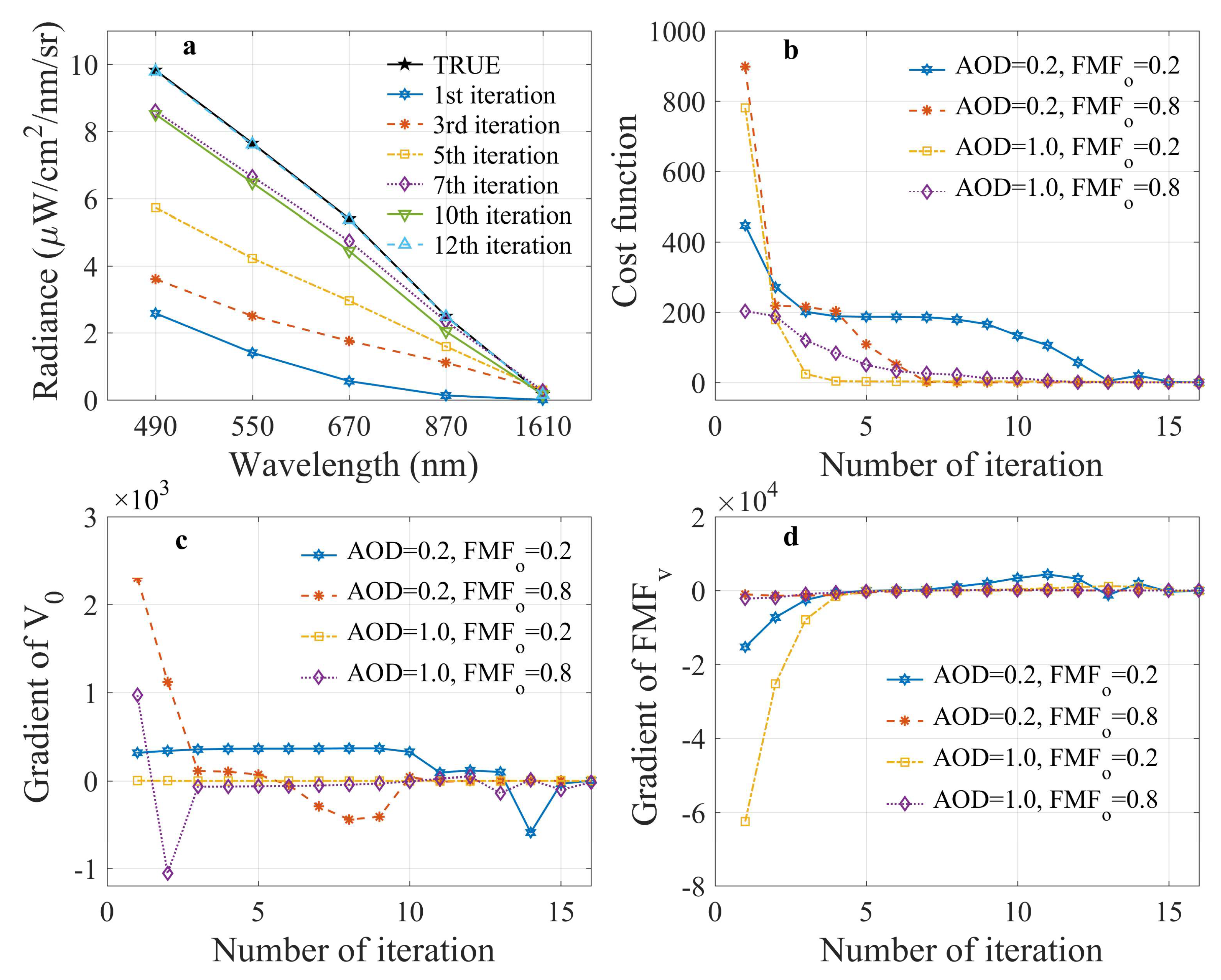
4.1. Retrieval from Synthetic Data
4.2. Retrieval from Experimental Data
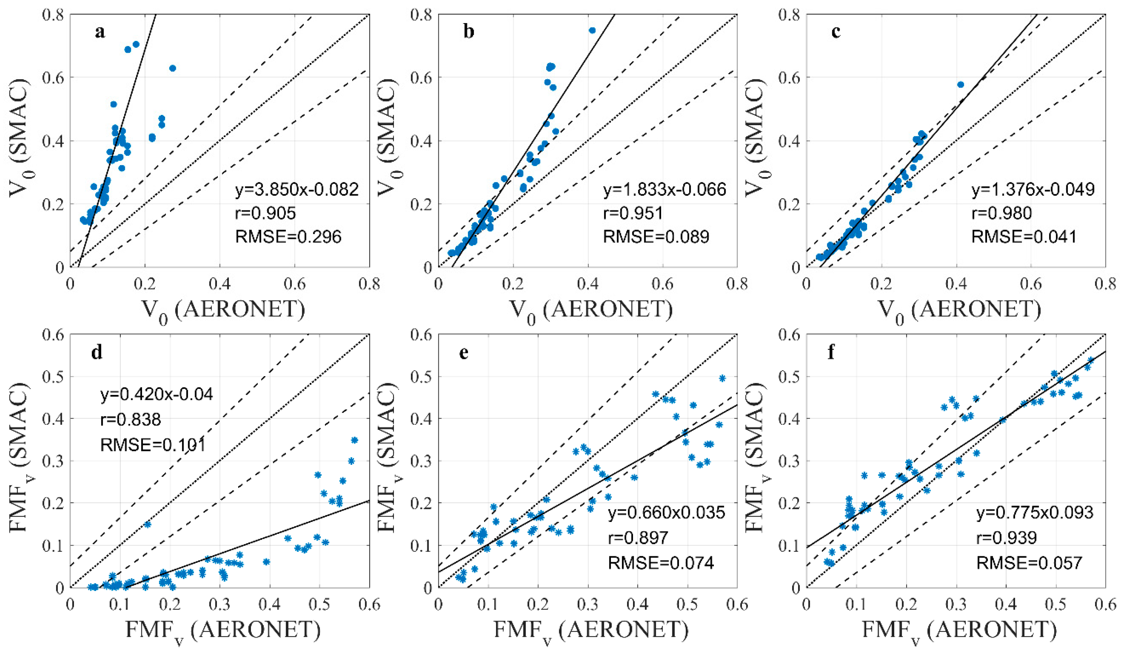
4.2.1. Validation of V0 and FMFv
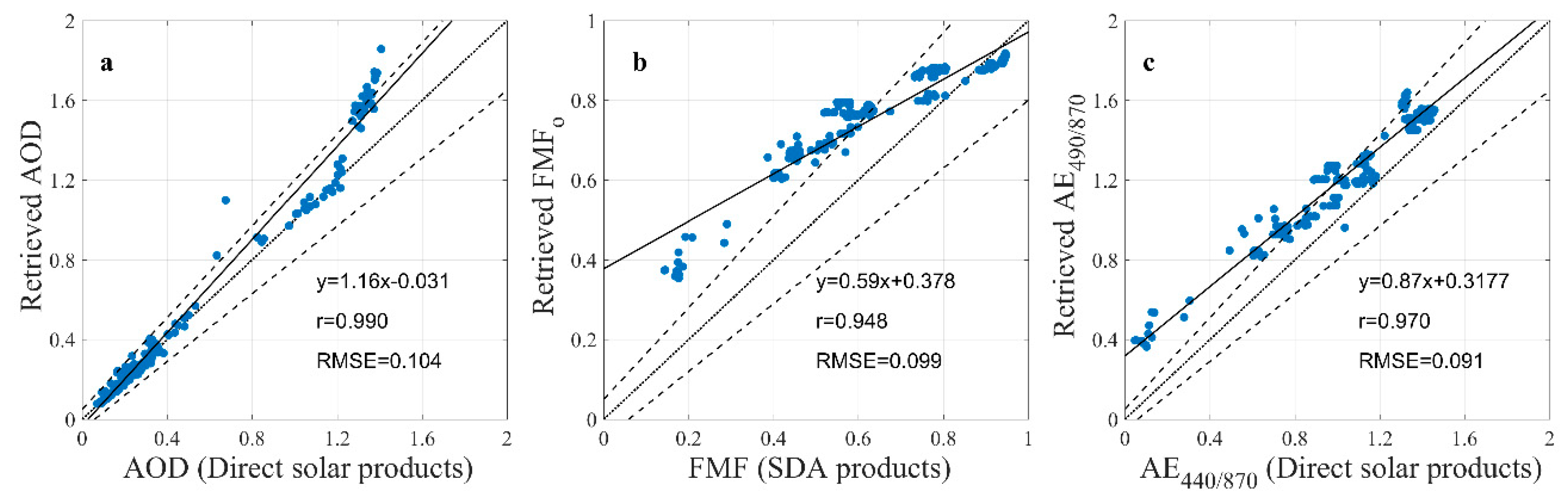
4.2.2. Validation of AOD and FMFo
4.2.3. Fitting Residuals
5. Discussion
5.1. The Limit of the Algorithm
5.2. Application Potential
6. Conclusions
Author Contributions
Funding
Acknowledgments
Conflicts of Interest
References
- Dockery, D.W.; Rd, P.C.; Xu, X.; Spengler, J.D.; Ware, J.H.; Fay, M.E.; Ferris, B.G., Jr.; Speizer, F.E. An association between air pollution and mortality in six U.S. Cities. New Engl. J. Med. 1993, 329, 1753–1759. [Google Scholar] [CrossRef] [PubMed]
- Kaufman, Y.J.; Boucher, O.; Tanré, D.; Chin, M.; Remer, L.A.; Takemura, T. Aerosol anthropogenic component estimated from satellite data. Geophys. Res. Lett. 2005, 32, 317–330. [Google Scholar] [CrossRef]
- Hoek, G.; Krishnan, R.M.; Beelen, R.; Peters, A.; Ostro, B.; Brunekreef, B.; Kaufman, J.D. Long-term air pollution exposure and cardio- respiratory mortality: A review. Environ. Health 2013, 12, 43. [Google Scholar] [CrossRef] [PubMed]
- Cohen, A.J.; Brauer, M.; Burnett, R.; Anderson, H.R.; Frostad, J.; Estep, K.; Balakrishnan, K.; Brunekreef, B.; Dandona, L.; Dandona, R. Estimates and 25-year trends of the global burden of disease attributable to ambient air pollution: An analysis of data from the global burden of diseases study 2015. Lancet 2017, 389, 1907–1918. [Google Scholar] [CrossRef]
- Seaton, A.; Godden, D.; Macnee, W.; Donaldson, K. Particulate air pollution and acute health effects. Lancet 1995, 345, 176–178. [Google Scholar] [CrossRef]
- Song, C.; He, J.; Wu, L.; Jin, T.; Chen, X.; Li, R.; Ren, P.; Zhang, L.; Mao, H. Health burden attributable to ambient PM2.5 in china. Environ. Pollut. 2017, 223, 575. [Google Scholar] [CrossRef]
- Zhang, Y.; Li, Z. Remote sensing of atmospheric fine particulate matter (PM2.5) mass concentration near the ground from satellite observation. Remote Sens. Environ. 2015, 160, 252–262. [Google Scholar] [CrossRef]
- Li, Z.; Zhang, Y.; Shao, J.; Li, B.; Hong, J.; Liu, D.; Li, D.; Wei, P.; Li, W.; Li, L.; et al. Remote sensing of atmospheric particulate mass of dry PM2.5 near the ground: Method validation using ground-based measurements. Remote Sens. Environ. 2016, 173, 59–68. [Google Scholar] [CrossRef]
- Li, Z.; Wei, Y.; Zhang, Y.; Xie, Y.; Li, L.; Li, K.; Ma, Y.; Sun, X.; Zhao, W.; Gu, X. Retrieval of atmospheric fine particulate density based on merging particle size distribution measurements: Multi-instrument observation and quality control at shouxian. J. Geophys. Res. Atmos. 2018, 123, 12–474. [Google Scholar] [CrossRef]
- Yan, X.; Shi, W.Z.; Li, Z.Q.; Li, Z.Q.; Luo, N.N.; Zhao, W.J.; Wang, H.F.; Yu, X. Satellite-based PM2.5 estimation using fine-mode aerosol optical thickness over china. Atmos. Environ. 2017, 170, 290–302. [Google Scholar] [CrossRef]
- Zhang, Y.; Li, Z.; Qie, L.; Zhang, Y.; Liu, Z.; Chen, X.; Hou, W.; Li, K.; Li, D.; Xu, H. Retrieval of aerosol fine-mode fraction from intensity and polarization measurements by parasol over east asia. Remote Sens. 2016, 8, 417. [Google Scholar] [CrossRef]
- Kaufman, Y.J.; Wald, A.E.; Remer, L.A.; Bo-Cai, G.; Rong-Rong, L.; Flynn, L. The modis 2.1-μm channel-correlation with visible reflectance for use in remote sensing of aerosol. IEEE Trans. Geosci. Remote Sens. 1997, 35, 1286–1298. [Google Scholar] [CrossRef]
- Levy, R.C.; Remer, L.A.; Mattoo, S.; Vermote, E.F.; Kaufman, Y.J. Second-generation operational algorithm: Retrieval of aerosol properties over land from inversion of moderate resolution imaging spectroradiometer spectral reflectance. J. Geophys. Res. Atmos. 2007, 112. [Google Scholar] [CrossRef]
- Levy, R.C.; Remer, L.A.; Kleidman, R.G.; Mattoo, S.; Ichoku, C.; Kahn, R.; Eck, T.F. Global evaluation of the collection 5 modis dark-target aerosol products over land. Atmos. Chem. Phys. 2010, 10, 10399–10420. [Google Scholar] [CrossRef]
- Zhao, A.; Li, Z.; Zhang, Y.; Zhang, Y.; Li, D. Merging modis and ground-based fine mode fraction of aerosols based on the geostatistical data fusion method. Atmosphere 2017, 8, 117. [Google Scholar] [CrossRef]
- Dubovik, O.; Herman, M.; Holdak, A.; Lapyonok, T.; Tanré, D.; Deuzé, J.L.; Ducos, F.; Sinyuk, A.; Lopatin, A. Statistically optimized inversion algorithm for enhanced retrieval of aerosol properties from spectral multi-angle polarimetric satellite observations. Atmos. Meas. Tech. 2011, 4, 975–1018. [Google Scholar] [CrossRef]
- Waquet, F.; Cornet, C.; Deuzé, J.L.; Dubovik, O.; Ducos, F.; Goloub, P.; Herman, M.; Lapyonok, T.; Labonnote, L.C.; Riedi, J.; et al. Retrieval of aerosol microphysical and optical properties above liquid clouds from polder/parasol polarization measurements. Atmos. Meas. Tech. 2013, 6, 991–1016. [Google Scholar] [CrossRef]
- Zhang, Y.; Li, Z.; Qie, L.; Hou, W.; Liu, Z.; Zhang, Y.; Xie, Y.; Chen, X.; Xu, H. Retrieval of aerosol optical depth using the empirical orthogonal functions (eofs) based on parasol multi-angle intensity data. Remote Sens. 2017, 9, 578. [Google Scholar] [CrossRef]
- Lolli, S.; Madonna, F.; Rosoldi, M.; Campbell, J.R.; Welton, E.J.; Lewis, J.R.; Gu, Y.; Pappalardo, G. Impact of varying lidar measurement and data processing techniques in evaluating cirrus cloud and aerosol direct radiative effects. Atmos. Meas. Tech. 2018, 11, 1639–1651. [Google Scholar] [CrossRef]
- O’Neill, N.T.; Eck, T.F.; Smirnov, A.; Holben, B.N.; Thulasiraman, S. Spectral discrimination of coarse and fine mode optical depth. J. Geophys. Res. Atmos. 2003, 108. [Google Scholar] [CrossRef]
- Holben, B.N.; Eck, T.F.; Slutsker, I.; Tanré, D.; Buis, J.P.; Setzer, A.; Vermote, E.; Reagan, J.A.; Kaufman, Y.J.; Nakajima, T.; et al. Aeronet—A federated instrument network and data archive for aerosol characterization. Remote Sens. Environ. 1998, 66, 1–16. [Google Scholar] [CrossRef]
- Dubovik, O.; King, M.D. A flexible inversion algorithm for retrieval of aerosol optical properties from sun and sky radiance measurements. J. Geophys. Res. Atmos. 2000, 105, 20673–20696. [Google Scholar] [CrossRef]
- Knobelspiesse, K.; Cairns, B.; Mishchenko, M.; Chowdhary, J.; Tsigaridis, K.; Van, D.B.; Martin, W.; Ottaviani, M.; Alexandrov, M. Analysis of fine-mode aerosol retrieval capabilities by different passive remote sensing instrument designs. Opt. Express 2012, 20, 21457–21484. [Google Scholar] [CrossRef]
- Li, Z.; Hou, W.; Hong, J.; Zheng, F.; Luo, D.; Wang, J.; Gu, X.; Qiao, Y. Directional polarimetric camera (dpc): Monitoring aerosol spectral optical properties over land from satellite observation. J. Quant. Spectrosc. Radiat. Transf. 2018, 218, 21–37. [Google Scholar] [CrossRef]
- Dubovik, O.; Li, Z.; Mishchenko, M.I.; Tanr¨¦, D.; Karol, Y.; Bojkov, B.; Cairns, B.; Diner, D.J.; Espinosa, W.R.; Goloub, P.; et al. Polarimetric remote sensing of atmospheric aerosols: Instruments, methodologies, results, and perspectives. J. Quant. Spectrosc. Radiat. Transf. 2019, 224, 474–511. [Google Scholar] [CrossRef]
- Kokhanovsky, A.A. The modern aerosol retrieval algorithms based on the simultaneous measurements of the intensity and polarization of reflected solar light: A review. Front. Environ. Sci. 2015, 3, 4. [Google Scholar] [CrossRef]
- Li, Z.Q.; Xu, H.; Li, K.T.; Li, D.H.; Xie, Y.S.; Li, L.; Zhang, Y.; Gu, X.F.; Zhao, W.; Tian, Q.J.; et al. Comprehensive study of optical, physical, chemical, and radiative properties of total columnar atmospheric aerosols over china: An overview of sun–sky radiometer observation network (sonet) measurements. Bull. Am. Meteorol. Soc. 2018, 99, 739–755. [Google Scholar] [CrossRef]
- Hou, W.; Li, Z.; Wang, J.; Xu, X.; Goloub, P.; Qie, L. Improving remote sensing of aerosol microphysical properties by near-infrared polarimetric measurements over vegetated land: Information content analysis. J. Geophys. Res. Atmos. 2018, 123, 2215–2243. [Google Scholar] [CrossRef]
- Rodgers, C.D. Inverse Methods for Atmospheric Sounding: Theory and Practice; World Scientific: Singapore, 2000. [Google Scholar]
- Waquet, F.; Cairns, B.; Knobelspiesse, K.; Chowdhary, J.; Travis, L.D.; Schmid, B.; Mishchenko, M.I. Polarimetric remote sensing of aerosols over land. J. Geophys. Res. Atmos. 2009, 114. [Google Scholar] [CrossRef]
- Xu, X.; Wang, J.; Zeng, J.; Spurr, R.; Liu, X.; Dubovik, O.; Li, L.; Li, Z.; Mishchenko, M.I.; Siniuk, A.; et al. Retrieval of aerosol microphysical properties from aeronet photopolarimetric measurements: 2. A new research algorithm and case demonstration. J. Geophys. Res. Atmos. 2015, 120, 7079–7098. [Google Scholar] [CrossRef]
- Xu, X.; Wang, J.; Henze, D.K.; Qu, W.; Kopacz, M. Constraints on aerosol sources using geos-chem adjoint and modis radiances, and evaluation with multisensor (omi, misr) data. J. Geophys. Res. Atmos. 2013, 118, 6396–6413. [Google Scholar] [CrossRef]
- Anderson, T.L.; Wu, Y.; Chu, D.A.; Schmid, B.; Redemann, J.; Dubovik, O. Testing the modis satellite retrieval of aerosol fine-mode fraction. J. Geophys. Res. Atmos. 2005, 110. [Google Scholar] [CrossRef]
- Anderson, T.L.; Masonis, S.J.; Covert, D.S.; Ahlquist, N.C.; Howell, S.G.; Clarke, A.D.; Mcnaughton, C.S. Variability of aerosol optical properties derived from in situ aircraft measurements during ACE-Asia. J. Geophys. Res. Atmos. 2003, 108. [Google Scholar] [CrossRef]
- Kleidman, R.G.; O’Neill, N.T.; Remer, L.A.; Kaufman, Y.J.; Eck, T.F.; Tanré, D.; Dubovik, O.; Holben, B.N. Comparison of moderate resolution imaging spectroradiometer (modis) and aerosol robotic network (aeronet) remote-sensing retrievals of aerosol fine mode fraction over ocean. J. Geophys. Res. Atmos. 2005, 110. [Google Scholar] [CrossRef]
- Zhang, Y.; Li, Z.; Zhang, Y.; Li, D.; Qie, L.; Che, H.; Xu, H. Estimation of aerosol complex refractive indices for both fine and coarse modes simultaneously based on aeronet remote sensing products. Atmos. Meas. Tech. 2017, 10, 3203–3213. [Google Scholar] [CrossRef]
- Liu, Z.; Mortier, A.; Li, Z.; Hou, W.; Goloub, P.; Lv, Y.; Chen, X.; Li, D.; Li, K.; Xie, Y. Improving daytime planetary boundary layer height determination from caliop: Validation based on ground-based lidar station. Adv. Meteorol. 2017, 2017, 1–14. [Google Scholar] [CrossRef]
- Zhang, W.; Guo, J.; Miao, Y.; Liu, H.; Zhang, Y.; Li, Z.; Zhai, P. Planetary boundary layer height from caliop compared to radiosonde over china. Atmos. Chem. Phys. 2016, 16, 9951–9963. [Google Scholar] [CrossRef]
- Wang, J.; Xu, X.; Ding, S.; Zeng, J.; Spurr, R.; Liu, X.; Chance, K.; Mishchenko, M. A numerical testbed for remote sensing of aerosols, and its demonstration for evaluating retrieval synergy from a geostationary satellite constellation of geo-cape and goes-r. J. Quant. Spectrosc. Radiat. Transf. 2014, 146, 510–528. [Google Scholar] [CrossRef]
- Xu, X.; Wang, J. Retrieval of aerosol microphysical properties from aeronet photopolarimetric measurements: 1. Information content analysis. J. Geophys. Res. Atmos. 2015, 120, 7059–7078. [Google Scholar] [CrossRef]
- Hou, W.; Wang, J.; Xu, X.; Reid, J.S.; Han, D. An algorithm for hyperspectral remote sensing of aerosols: 1. Development of theoretical framework. J. Quant. Spectrosc. Radiat. Transf. 2016, 178, 400–415. [Google Scholar] [CrossRef]
- Hou, W.; Wang, J.; Xu, X.; Reid, J.S. An algorithm for hyperspectral remote sensing of aerosols: 2. Information content analysis for aerosol parameters and principal components of surface spectra. J. Quant. Spectrosc. Radiat. Transf. 2017, 192, 14–29. [Google Scholar] [CrossRef]
- Hou, W.Z.; Li, Z.Q.; Zheng, F.X.; Qie, L.L. Retrieval of aerosol microphysical properties based on the optimal estimation method: Information content analysis for satellite polarimetric remote sensing measurements. In ISPRS - International Archives of the Photogrammetry, Remote Sensing and Spatial Information Sciences; 2018; pp. 533–537. [Google Scholar]
- Luenberger, D.G.; Ye, Y. Linear and nonlinear programming. Int. Encycl. Soc. Behav. Sci. 2004, 67, 8868–8874. [Google Scholar]
- Yu, J.; Li, M.; Wang, Y.; He, G. A decomposition method for large-scale box constrained optimization. Appl. Math. Comput. 2014, 231, 9–15. [Google Scholar] [CrossRef]
- Zhu, C.; Byrd, R.H.; Lu, P.; Nocedal, J. A Limited Memory Fortran Code for Solving Bound Constrained Optimization Problems. Technique Report, Northwestern Univ. 1994. [Google Scholar]
- Byrd, R.H.; Lu, P.; Nocedal, J.; Zhu, C. A limited memory algorithm for bound constrained optimization. SIAM J. Sci. Comput. 1995, 16, 1190–1208. [Google Scholar] [CrossRef]
- Xiao, Y.; Zhang, H. Modified subspace limited memory bfgs algorithm for large-scale bound constrained optimization. J. Comput. Appl. Math. 2008, 222, 429–439. [Google Scholar] [CrossRef]
- Che, H.; Xia, X.; Zhu, J.; Wang, H.; Wang, Y.; Sun, J.; Zhang, X.; Shi, G. Aerosol optical properties under the condition of heavy haze over an urban site of beijing, china. Environ. Sci. Pollut. Res. 2015, 22, 1043–1053. [Google Scholar] [CrossRef] [PubMed]
- Ou, Y.; Zhao, W.H.; Wang, J.Q.; Zhao, W.J.; Zhang, B. Characteristics of aerosol types in beijing and the associations with air pollution from 2004 to 2015. Remote Sens. 2017, 9, 19. [Google Scholar] [CrossRef]
- Torres, B.; Dubovik, O.; Fuertes, D.; Schuster, G.; Cachorro, V.E.; Lapyonok, T.; Goloub, P.; Blarel, L.; Barreto, A.; Mallet, M.; et al. Advanced characterisation of aerosol size properties from measurements of spectral optical depth using the grasp algorithm. Atmos. Meas. Tech. 2017, 10, 3743–3781. [Google Scholar] [CrossRef]
- Zheng, F.; Hou, W.; Li, Z. Optimal estimation retrieval for directional polarimetric camera onboard chinese gaofen-5 satellite: An analysis on multi-angle dependence and a posteriori error. Acta Phys. Sin. 2019, 68, 40701. [Google Scholar]


| Abbreviation | Distinction of definition | References |
|---|---|---|
| FMF | The fine-mode fraction (FMF) is defined optically and calculated by the optical spectral deconvolution algorithm (SDA) rather than intermediate computations of the aerosol particle size distribution (PSD) parameters and refractive indices. | [20] |
| The FMF is defined optically and retrieved independently by irrelevant aerosol model assumptions for total aerosol optical depth (AOD) and fine-mode AOD. | [11] | |
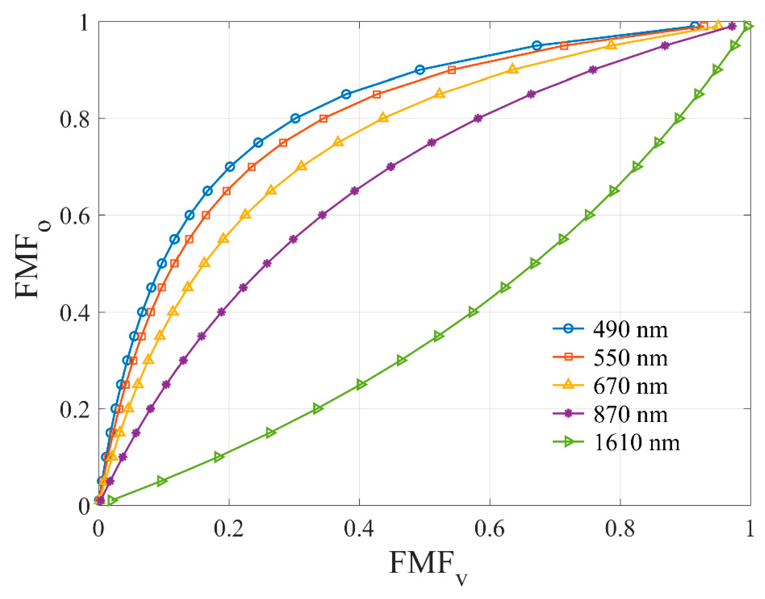
| FMFv/FMFo | The physical volume fine-mode fraction (FMFv)/optical fine-mode fraction (FMFo) is defined based on a physical model in which the fine and coarse components follow a unified bimodal aerosol model. The subscripts ‘v’ and ‘o’ denote volume FMF and optical FMF, respectively. | [22,28,31] |
| SMF | The SMF (Sub Micrometer Fraction) is defined in terms of a microphysical cutoff of the associated PSD at some specific radius. Two acquisition methods are available: (1) calculating using the cutoff radius based on the bimodal aerosol model; and (2) obtaining it by in situ measurement. The widely accepted cut-off radius is 0.6µm. | [33,34,35] |
| Mode | ||||
|---|---|---|---|---|
| Fine | 0.155 | 0.284 | 1.39, 1.40, 1.40, 1.42, 1.41 | 0.0079, 0.0075, 0.0066, 0.0066, 0.0067 |
| Coarse | 2.213 | 0.482 | 1.53, 1.54, 1.55, 1.54, 1.50 | 0.0049, 0.0041, 0.0023, 0.0019, 0.0009 |
| Name | Setting |
|---|---|
| Measurement vector | |
| Observation uncertainties | , ϵI = 5% (relative error) |
| State vector | V0 ≥ 0.001 μm3/μm2 |
| A priori estimates uncertainties | (relative error) |
| Parameters | Setting |
|---|---|
| Solar zenith angle (SZA) | 60° |
| View zenith angle (VZA) | 0° (vertical upward observation) |
| Relative azimuth angle (RAA) | 0° (solar principal plane) |
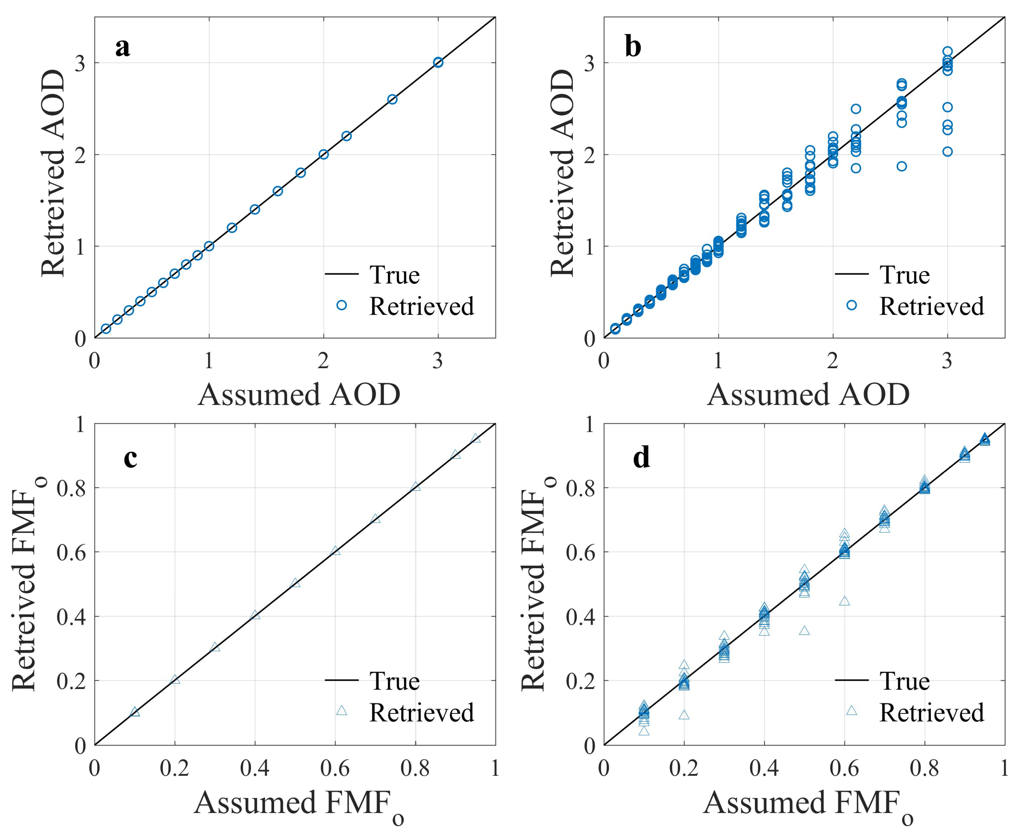
| Aerosol optical depth (AOD) at 550 nm | from 0.1–3.0 |
| Fine-mode fraction (FMFo) at 550 nm | from 0.1–0.95 |
© 2019 by the authors. Licensee MDPI, Basel, Switzerland. This article is an open access article distributed under the terms and conditions of the Creative Commons Attribution (CC BY) license (http://creativecommons.org/licenses/by/4.0/).
Share and Cite
Zheng, F.; Hou, W.; Sun, X.; Li, Z.; Hong, J.; Ma, Y.; Li, L.; Li, K.; Fan, Y.; Qiao, Y. Optimal Estimation Retrieval of Aerosol Fine-Mode Fraction from Ground-Based Sky Light Measurements. Atmosphere 2019, 10, 196. https://doi.org/10.3390/atmos10040196
Zheng F, Hou W, Sun X, Li Z, Hong J, Ma Y, Li L, Li K, Fan Y, Qiao Y. Optimal Estimation Retrieval of Aerosol Fine-Mode Fraction from Ground-Based Sky Light Measurements. Atmosphere. 2019; 10(4):196. https://doi.org/10.3390/atmos10040196
Chicago/Turabian StyleZheng, Fengxun, Weizhen Hou, Xiaobing Sun, Zhengqiang Li, Jin Hong, Yan Ma, Li Li, Kaitao Li, Yizhe Fan, and Yanli Qiao. 2019. "Optimal Estimation Retrieval of Aerosol Fine-Mode Fraction from Ground-Based Sky Light Measurements" Atmosphere 10, no. 4: 196. https://doi.org/10.3390/atmos10040196
APA StyleZheng, F., Hou, W., Sun, X., Li, Z., Hong, J., Ma, Y., Li, L., Li, K., Fan, Y., & Qiao, Y. (2019). Optimal Estimation Retrieval of Aerosol Fine-Mode Fraction from Ground-Based Sky Light Measurements. Atmosphere, 10(4), 196. https://doi.org/10.3390/atmos10040196