Spatio-Temporal Variability of the Precipitable Water Vapor over Peru through MODIS and ERA-Interim Time Series


Abstract
1. Introduction
2. Methodology
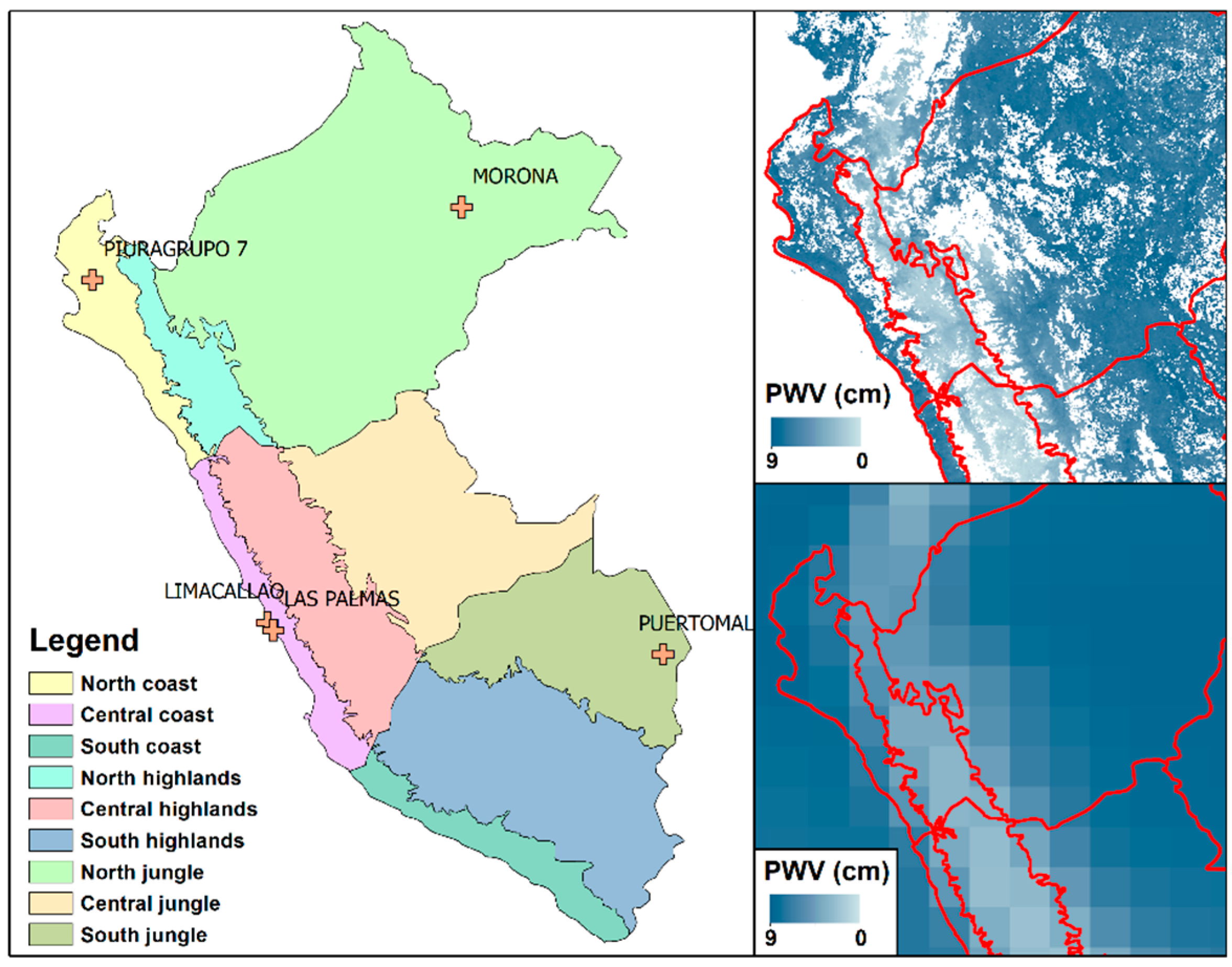
2.1. Study Area
2.2. Datasets
2.2.1. MODIS
2.2.2. ERA-Interim
2.2.3. Radiosonde
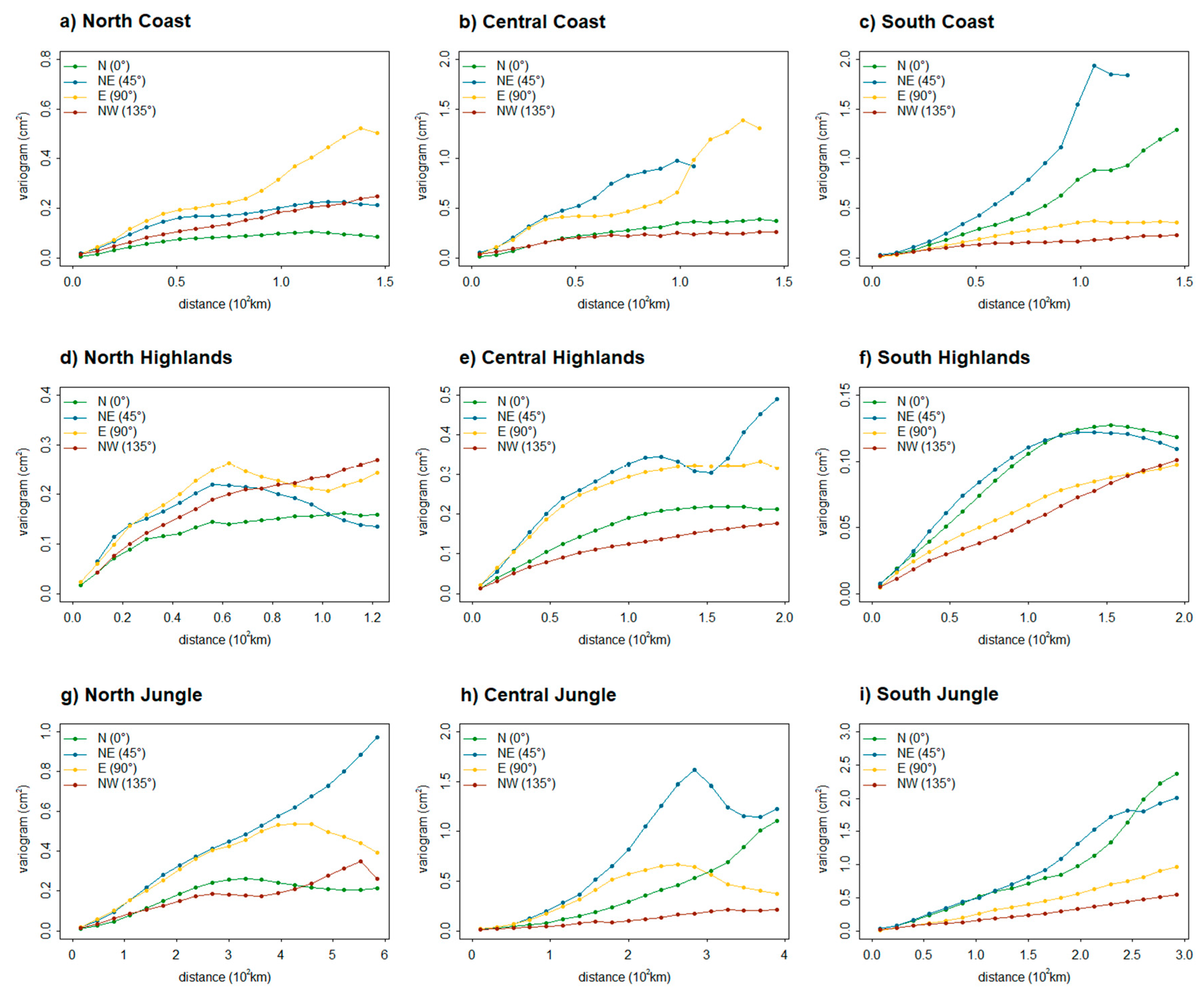
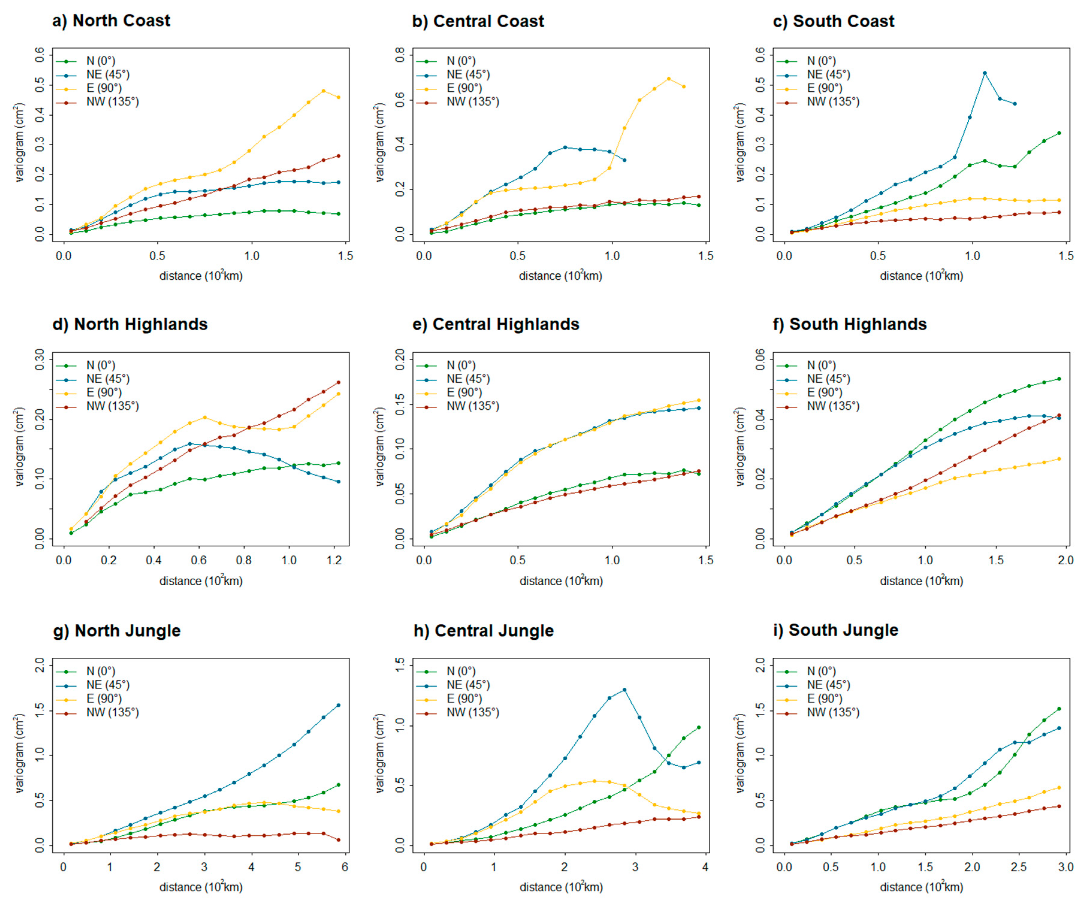
2.3. Spatial Analysis
2.4. Temporal Analysis
3. Results
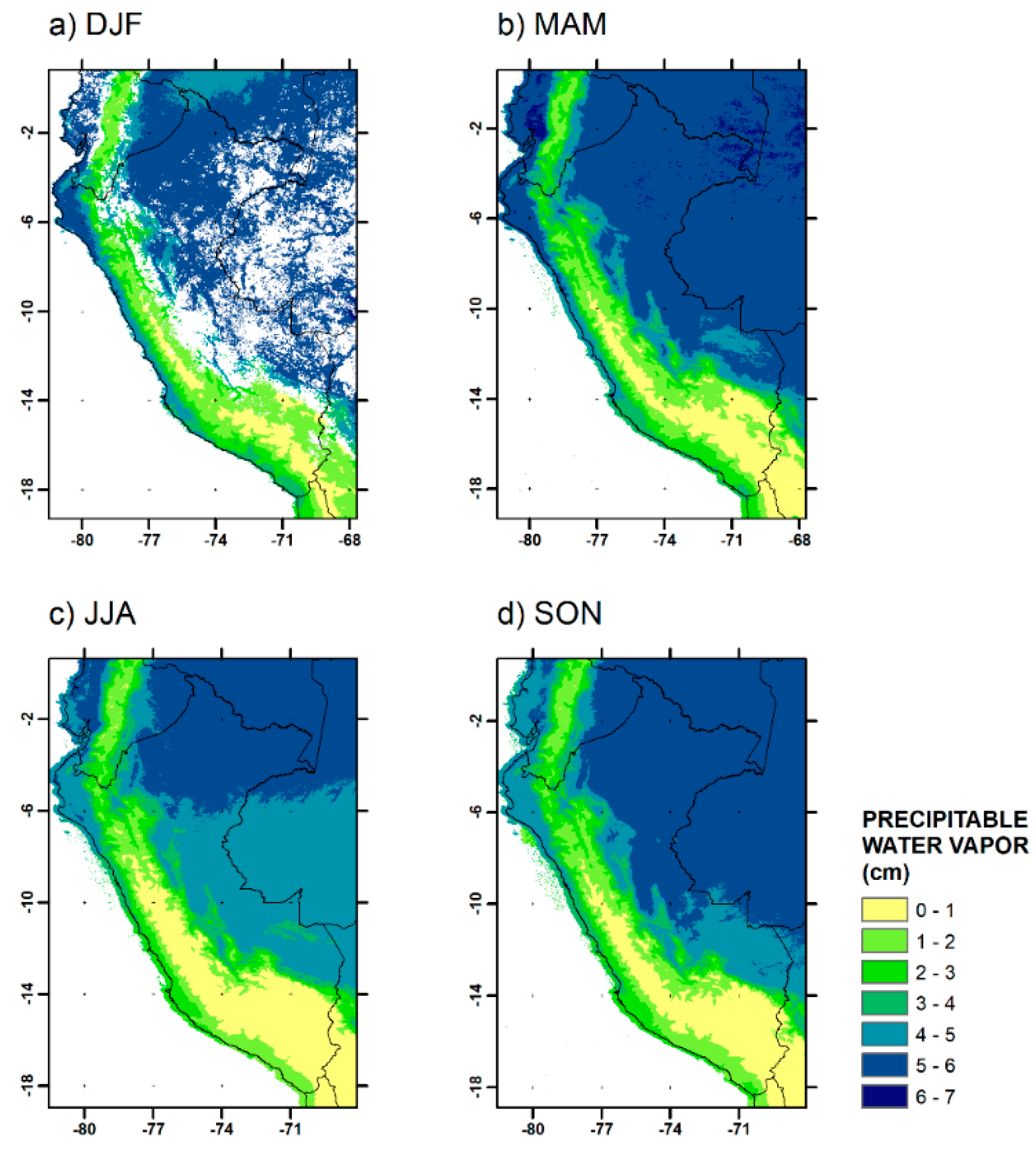
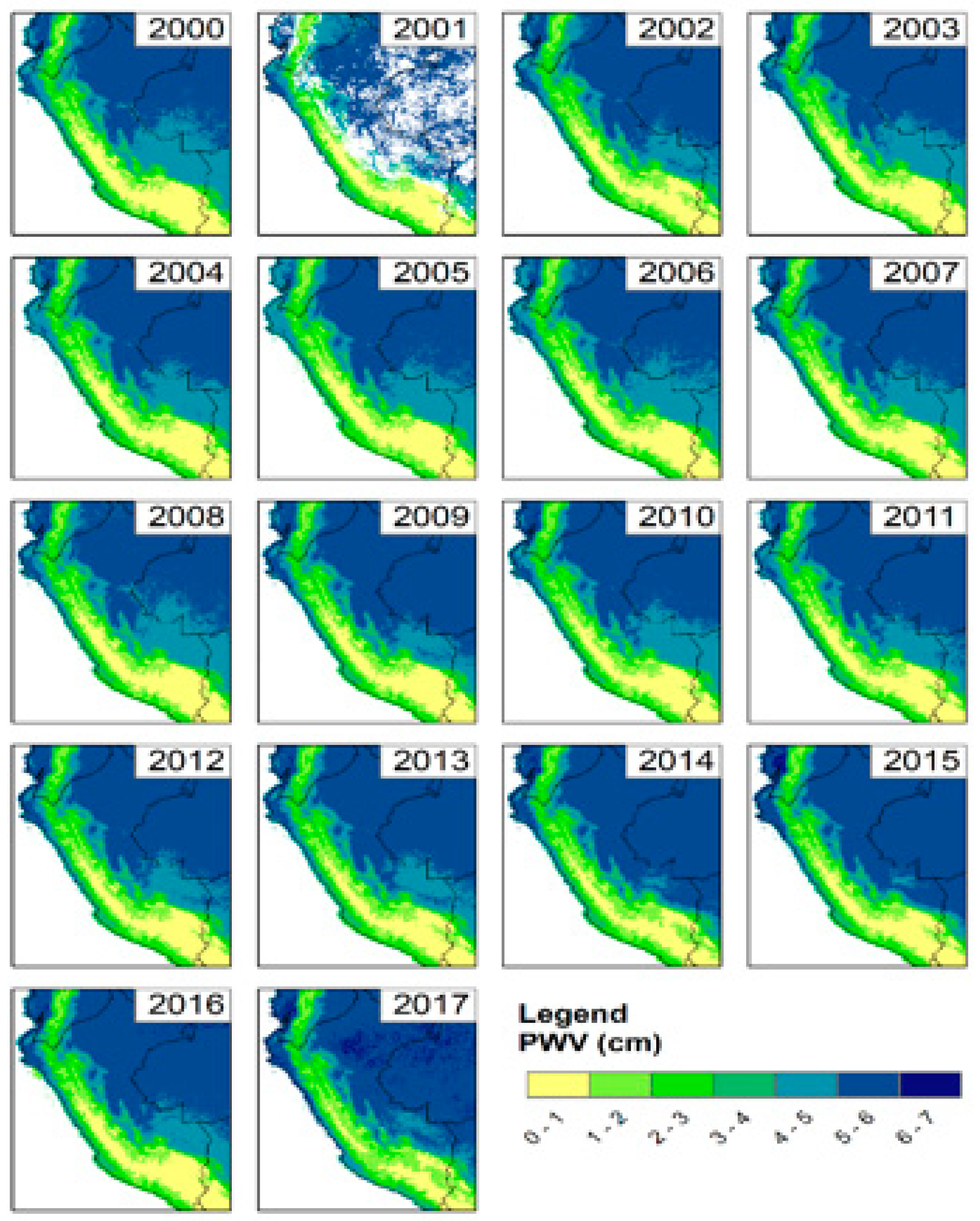
3.1. Spatial Analysis
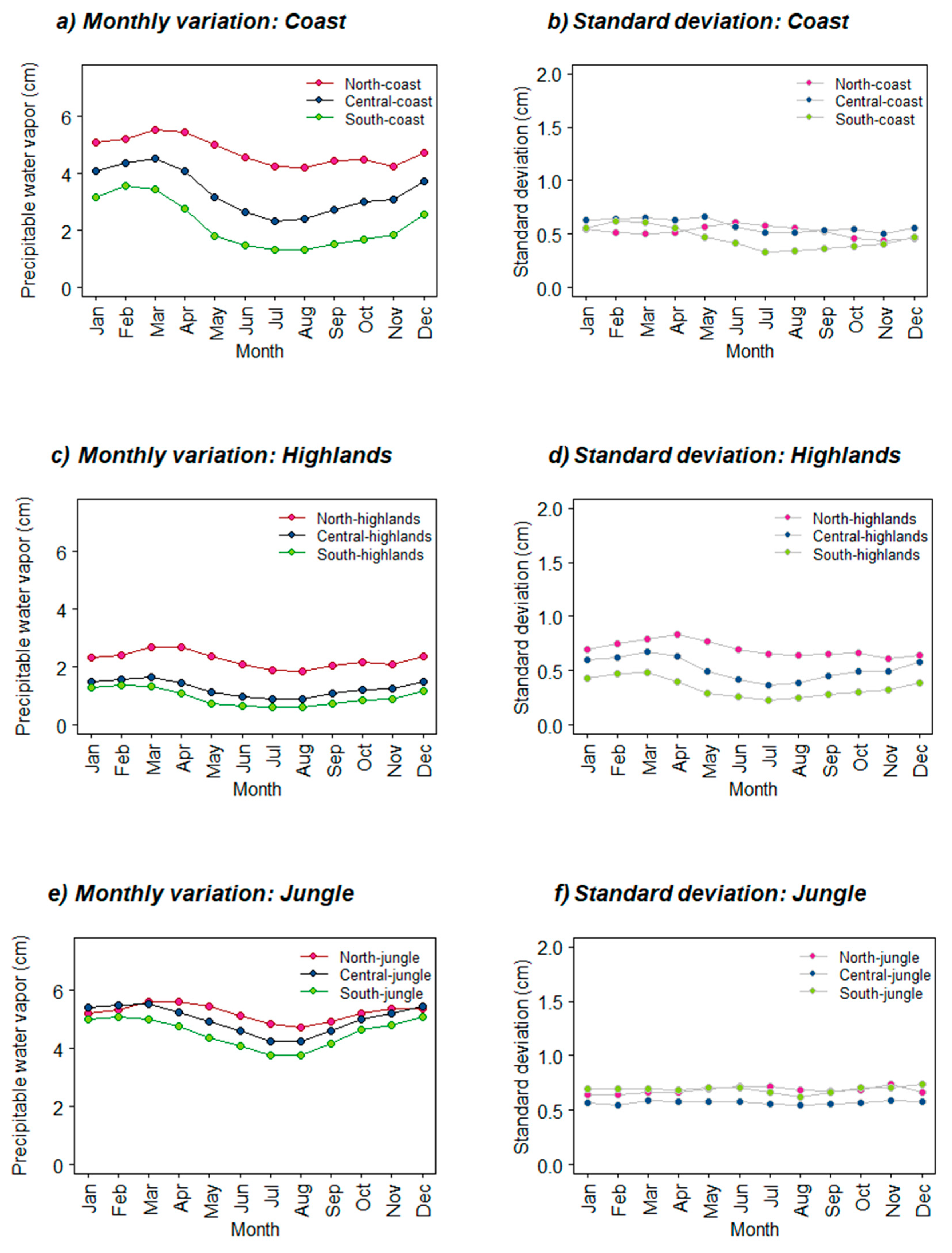
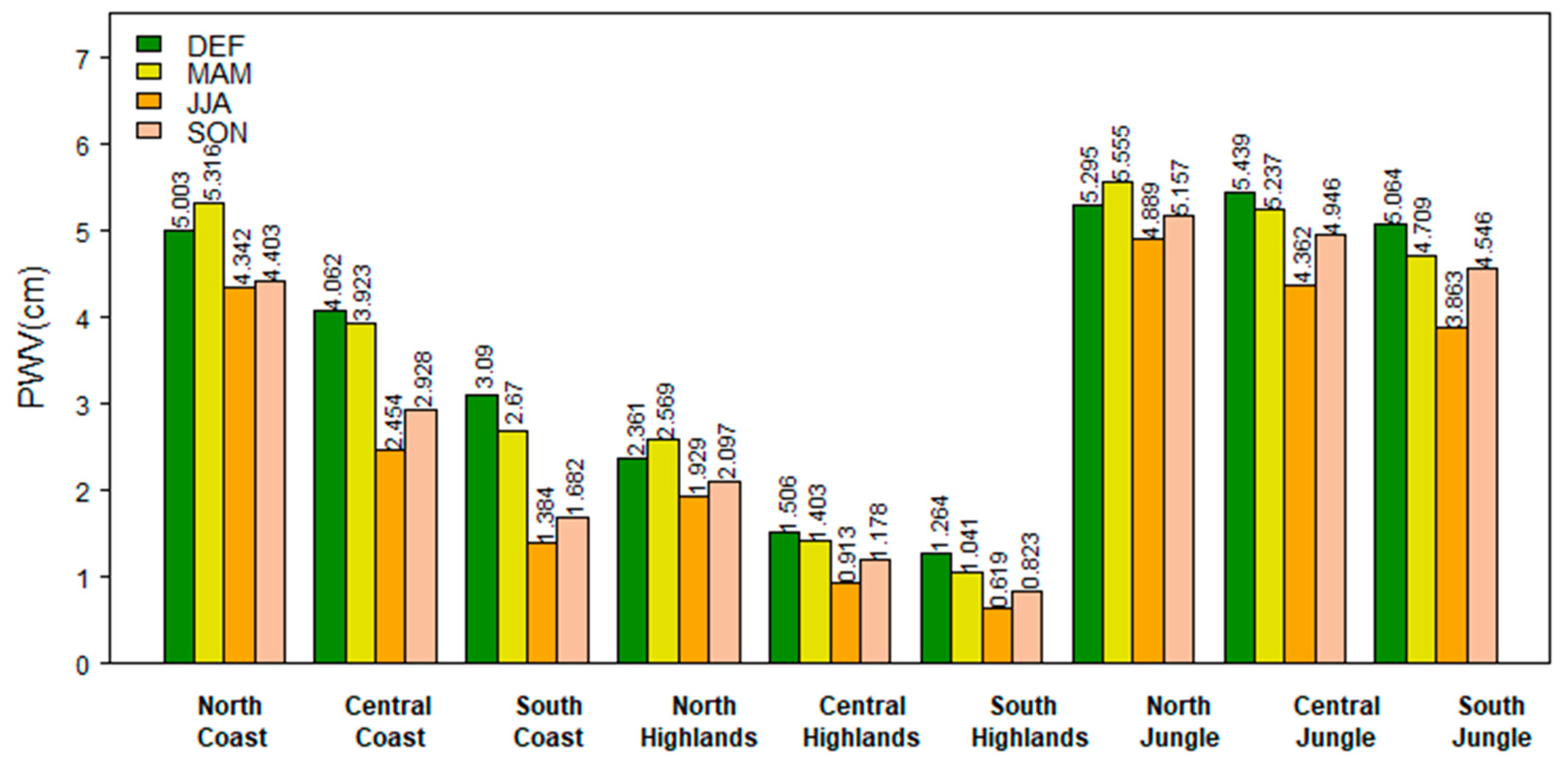
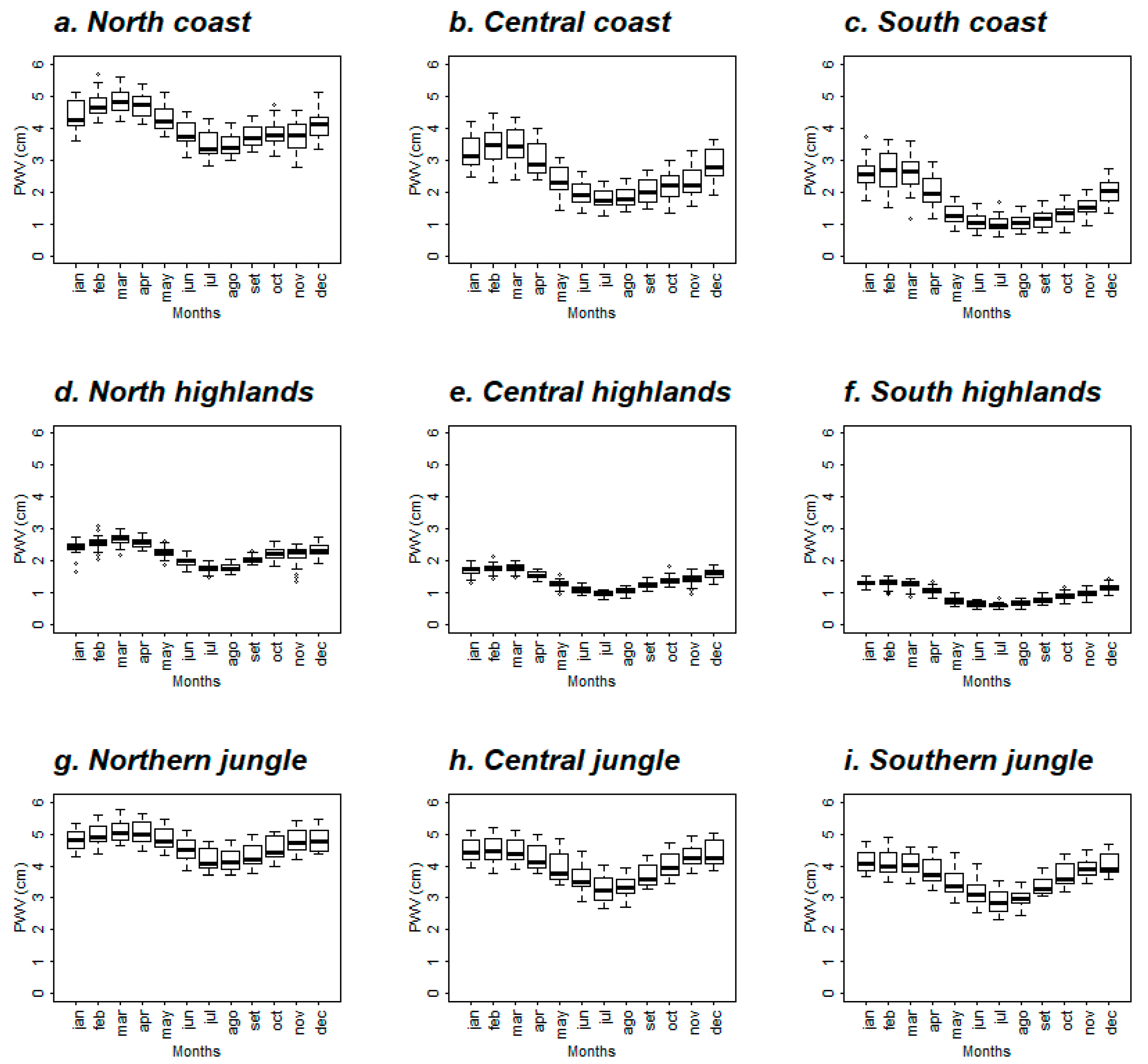
3.2. Temporal Analysis
3.3. Trend Analysis
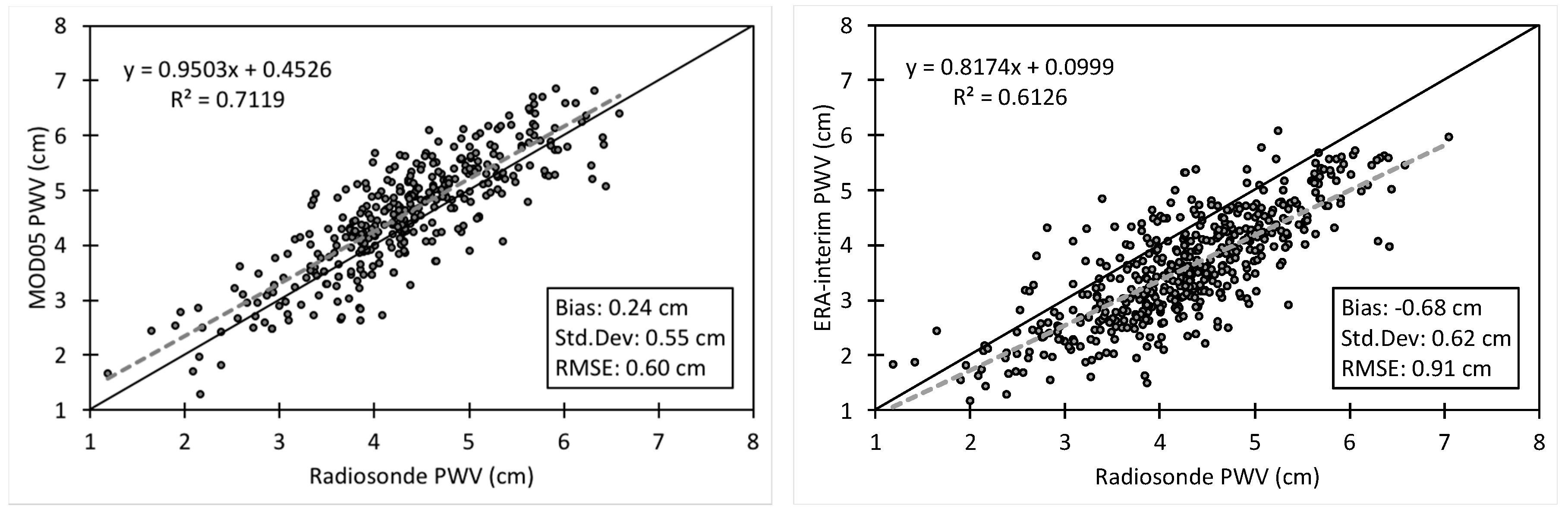
3.4. Validation against Radiosonde Data
4. Conclusions
Author Contributions
Funding
Acknowledgments
Conflicts of Interest
References
- Al-Mashagbah, A.; Al-Farajat, M. Assessment of Spatial and Temporal Variability of Rainfall Data Using Kriging, Mann Kendall Test and the Sen’s Slope Estimates in Jordan from 1980 to 2007. Res. J. Environ. Earth Sci. 2013, 5, 611–618. [Google Scholar]
- Arraut, J.M.; Satyamurty, P. Precipitation and water vapor transporting the Southern Hemisphere with emphasis on the South American region. J. Appl. Meteorol. Climatol. 2009, 48, 1902–1912. [Google Scholar] [CrossRef]
- Barnes, W.L.; Pagano, T.S.; Salomonson, V.V. Prelaunch Characteristics of the Moderate Resolution Imaging Spectroradiometer (MODIS) on EOS-AM1. IEEE Trans. Geosci. Remote Sens. 1998, 36, 1088–1100. [Google Scholar] [CrossRef]
- Berrisford, P.; Dee, D.; Fielding, K.; Fuentes, M.; Kallberg, P.; Kobayashi, S.; Uppala, S. The ERA-Interim Archive; ERA Report Series 1; ECMWF: Reading, UK, 2009; 16p. [Google Scholar]
- Berrisford, P.; Kallberg, P.; Kobayashi, S.; Dee, D.P.; Uppala, S.M.; Simmons, A.J.; Poli, P. Atmospheric Conservation Properties in ERA-Interim; ERA Report Series; ECMWF: Reading, UK, 2011. [Google Scholar]
- Burrough, P.A. Principles of Geographical Information Systems for Land Resources Assessment; Clarendon Press: Oxford, UK, 1986; 193p. [Google Scholar]
- Carvalho, J.R.P.; Vieira, S.R.; Grego, C.R. Comparação de métodos para ajuste de modelos de semivariograma da precipitação pluvial anual. Revista Brasileira de Engenharia Agrícola e Ambiental 2009, 13, 443–448. [Google Scholar] [CrossRef]
- Chang, L.; Gao, G.; Jin, S.; He, X.; Xiao, R.; Guo, L. Calibration and evaluation of precipitable water vapor from MODIS infrared observations at night. IEEE Trans. Geosci. Remote Sens. 2015, 53, 2612–2620. [Google Scholar] [CrossRef]
- Chebana, F.; Ouarda, T.B.M.J.; Duong, T.C. Testing for multivariate trends in hydrologic frequency analysis. J. Hydrol. 2013, 486, 519–530. [Google Scholar] [CrossRef]
- Clark, I. Regularization of a semivariogram. Comput. Geosci. 1977, 3, 341–346. [Google Scholar] [CrossRef]
- Cressie, N.A.C. Statistics for Spatial Data; John Wiley & Sons: New York, NY, USA, 1991; 900p. [Google Scholar]
- Dee, D.P.; Uppala, S.M.; Simmons, A.J.; Berrisford, P.; Poli, P.; Kobayashi, S.; Andrae, U.; Balmaseda, M.A.; Balsamo, G.; Bauer, P.; et al. The ERA-Interim reanalysis: Configuration and performance of the data assimilation system. Q. J. R. Meteorol. Soc. 2011, 137, 553–597. [Google Scholar] [CrossRef]
- Espinoza, J.C.; Ronchail, J.; Guyot, J.L.; Cochonneau, G.; Naziano, F.; Lavado, W.; Oliveira, E.; Pombosa, R.; Vauchel, P. Spatio-temporal rainfall variability in the Amazon basin countries (Brazil, Peru, Bolivia, Colombia, and Ecuador). Int. J. Climatol. 2009, 29, 1574–1594. [Google Scholar] [CrossRef]
- Fernández, L.I.; Meza, A.M.; Natali, M.P. Determinación del contenido de vapor de agua precipitable (PWV) a partir de mediciones GPS: Primeros resultados en Argentina. Geoacta 2009, 34, 35–57. [Google Scholar]
- Gao, B.C.; Kaufman, Y.J. The MODIS Near-IR Water Vapor Algorithm. 1998. Available online: https://modis-atmos.gsfc.nasa.gov/_docs/atbd_mod03.pdf (accessed on 7 April 2019).
- Gao, B.C.; Kaufman, Y.J. Water vapor retrievals using Moderate Resolution Imaging Spectroradiometer (MODIS) near-infrared channels. J. Geophys. Res. 2003, 108, 4389. [Google Scholar] [CrossRef]
- Liang, H.; Cao, Y.; Wan, X.; Xu, Z.; Wang, H.; Hu, H. Meteorological applications of precipitable water vapor measurements retrieved by the national GNSS network of China. Geod. Geodyn. 2015, 6, 135–142. [Google Scholar] [CrossRef]
- Journel, A.G.; Froidevaux, R. Anisotropic Hole-Effect Modeling. Math. Geol. 1982, 14, 217–247. [Google Scholar] [CrossRef]
- Kaufman, Y.J.; Gao, B.C. Remote sensing of water vapor in the near IR from EOS/MODIS. IEEE Trans. Geosci. Remote Sens. 1992, 30, 871–884. [Google Scholar] [CrossRef]
- Kendall, M.G. Rank Correlation Methods, 4th ed.; Charles Griffin: London, UK, 1975. [Google Scholar]
- King, M.D.; Kaufman, Y.J.; Menzel, W.P.; Tanré, D. Remote sensing of cloud, aerosol, and water vapor properties from the Moderate Resolution Imaging Spectrometer (MODIS). IEEE Trans. Geosci. Remote Sens. 1992, 30, 2–27. [Google Scholar] [CrossRef]
- King, M.D.; Herring, D.D.; Diner, D.J. The Earth Observing System: A Space-based Program for Assessing Mankind’s Impact on the Global Environment. Opt. Photonics News 1995, 6, 34–39. [Google Scholar] [CrossRef]
- King, M.D.; Menzel, W.P.; Kaufman, Y.J.; Tanré, D.; Gao, B.C.; Platnick, S.; Ackerman, S.A.; Remer, L.A.; Pincus, R.; Hubanks, P.A. Cloud and aerosol properties, precipitable water, and profiles of temperature and water vapor from MODIS. IEEE Trans. Geosci. Remote Sens. 2003, 41, 442–458. [Google Scholar] [CrossRef]
- Lara, C.; Miranda, M.; Montecino, V.; Iriarte, J.L. Chlorophyll-a MODIS mesoscale variability in the Inner Sea of Chiloé, Patagonia, Chile (41–43°S): Patches and Gradients? Revista de Biología Marina y Oceanografía 2010, 45, 217–225. [Google Scholar] [CrossRef]
- Longobardi, A.; Villani, P. Trend analysis of annual and seasonal rainfall time series in the Mediterranean area. Int. J. Climatol. 2010, 30, 1538–1546. [Google Scholar] [CrossRef]
- L’Heureux, M.L.; Takahashi, K.; Watkins, A.B.; Barnston, A.G.; Becker, E.J.; Di Liberto, T.E.; Gamble, F.; Gottschalck, J.; Halpert, M.S.; Huang, B.; et al. Observing and predicting the 2015–16 El Niño. Bull. Am. Meteorol. Soc. 2017, 98, 1363–1382. [Google Scholar] [CrossRef]
- Mann, H.B. Non-parametric Test against Trend. Econometrica 1945, 13, 245–259. [Google Scholar] [CrossRef]
- Marengo, J.A.; Nobre, C.A.; Tomasella, J.; Oyama, M.D.; Oliveira, G.S.; Oliveira, R.; Camargo, H.; Alves, L.M. The dought of Amazonia in 2005. J. Clim. 2008, 21, 495–516. [Google Scholar] [CrossRef]
- Matheron, G. Le Krigeage Universei; No. 1.; Cahiers de Centre de Morphologie Mathematique: Fontainbleau, France, 1969. [Google Scholar]
- Mattar, C.; Sobrino, J.A.; Julien, Y.; Morales, L. Trends in column integrated water vapour over Europe from 1973 to 2003. Int. J. Climatol. 2010, 31, 1749–1757. [Google Scholar] [CrossRef]
- Moreira, J.G.V.; Naghettini, M. Detecção de Tendências Monotônicas Temporais e Relação com Erros dos Tipos I e II: Estudo de Caso em Séries de Precipitações Diárias Máximas Anuais do Estado do Acre. Revista Brasileira de Meteorologia 2016, 31, 394–402. [Google Scholar] [CrossRef]
- Ning, T.; Wickert, J.; Deng, Z.; Heise, S.; Dick, G.; Vey, S.; Schöne, T. Homogenized time series of the atmospheric water vapor content obtained from the GNSS reprocessed data. J. Clim. 2016, 29, 2443–2456. [Google Scholar] [CrossRef]
- Platnick, S.; King, M.D.; Ackerman, S.A.; Menzel, W.P.; Baum, B.A.; Riédi, J.C.; Frey, R.A. The MODIS cloud products: Algorithms and examples from Terra. IEEE Trans. Geosci. Remote Sens. 2003, 41, 459–473. [Google Scholar] [CrossRef]
- Salati, E.; Marques, J.; Molion, L.C.B. Origem e distribuição das chuvas na Amazônia. Interciência 1978, 3, 200–206. [Google Scholar]
- Salomonson, V.V.; Barnes, W.L.; Maymon, P.W.; Montgomery, H.E.; Ostrow, H. MODIS: Advanced facility instrument for studies of the Earth as a system. IEEE Trans. Geosci. Remote Sens. 1989, 27, 145–153. [Google Scholar] [CrossRef]
- Simmons, A.; Uppala, S.; Dee, D.; Kobayashi, S. ERA-Interim: New ECMWF reanalysis products from 1989 onwards. ECMWF Newsl. 2007, 110, 25–35. [Google Scholar]
- Sobrino, J.A.; El Kharraz, J.; Li, Z.-L. Surface temperature and water vapour retrieval from MODIS data. Int. J. Remote Sens. 2003, 24, 5161–5182. [Google Scholar] [CrossRef]
- Russ, J.C. The Image Processing Handbook; CRC Press—IEEE Press: Piscataway, NJ, USA, 1998. [Google Scholar]
- Wang, H.; Wei, M.; Li, G.; Zhou, S.; Zeng, Q. Analysis of precipitable water vapor from GPS measurements in Chengdu region: Distribution and evolution characteristics in autumn. Adv. Space Res. 2013, 52, 656–667. [Google Scholar] [CrossRef]
- Wang, Y.; Yang, K.; Pan, Z.; Qin, J.; Chen, D.; Lin, C.; Chen, Y.; Zhu, L.; Tang, W.; Han, M.; et al. Evaluation of precipitable water vapor from four satellite products and four reanalysis datasets against GPS measurements on the southern Tibetan Plateau. J. Clim. 2017, 30, 5699–5713. [Google Scholar] [CrossRef]
- Wilks, D.S. Statistical Methods in the Atmospheric Sciences; Elsevier/Academic Press: Amsterdam, The Netherlands, 2011; 699p. [Google Scholar]
- Woodcock, C.E.; Strahler, A.H.; Jupp, D.L.B. The use of variograms in remote sensing: I. Scene models and simulated images. Remote Sens. Environ. 1988, 25, 323–348. [Google Scholar] [CrossRef]


| Station | Station Name | Latitude | Longitude | Time of Measurement | Data Period | |||
|---|---|---|---|---|---|---|---|---|
| 0 | 6 | 12 | 18 | |||||
| 84378 | MORONA | 03°44′ S | 73°15′ W | X | 2003–2010 * | |||
| 84416 | PIURA GRUPO 7 | 05°11′ S | 80°36′ W | X | 2003–2011 ** | |||
| 84628 | LIMA/CALLAO | 12°00′ S | 77°07′ W | X | X | X | X | 2009–2010 * |
| 84629 | LAS PALMAS | 12°09′ S | 77°00′ W | X | X | X | 2004–2005 * | |
| 84659 | PUERTO MALDONADO BAMAL | 12°38′ S | 69°14′ W | X | 2000–2016 *** | |||
| Subregion | Min | Percentile 1 | Median | Mean | Percentile 3 | Max |
|---|---|---|---|---|---|---|
| North Coast | 1 | 90.211 | 161.81 | 190.63 | 268.62 | 631.62 |
| Central Coast | 1 | 101.42 | 229.79 | 262.57 | 396.55 | 755.48 |
| South Coast | 1 | 97.306 | 201.74 | 231.11 | 340.23 | 702.68 |
| North Highland | 1 | 79.321 | 139.15 | 162.36 | 228.14 | 528.11 |
| Central Highland | 1 | 112.871 | 216.15 | 248.93 | 362.56 | 753.94 |
| South Highland | 1 | 148.06 | 237.05 | 256.19 | 347.93 | 751.63 |
| North Jungle | 1 | 219.56 | 345.18 | 360.69 | 482.35 | 1055.12 |
| Central Jungle | 1 | 129.8 | 219.01 | 232.98 | 322.85 | 705.76 |
| South Jungle | 1 | 110.55 | 173.91 | 187.11 | 248.71 | 594.66 |
| Month | North Coast | Central Coast | South Coast | North High | Central High | South High | North Jungle | Central Jungle | South Jungle |
|---|---|---|---|---|---|---|---|---|---|
| Jan | 0.111 | 0.425 | 1.562 | 0.140 | 0.215 | 0.122 | 0.220 | 0.462 | 1.317 |
| Feb | 0.098 | 0.524 | 1.886 | 0.158 | 0.252 | 0.131 | 0.255 | 0.469 | 1.364 |
| Mar | 0.105 | 0.500 | 1.417 | 0.179 | 0.279 | 0.124 | 0.284 | 0.528 | 1.215 |
| Apr | 0.085 | 0.335 | 0.768 | 0.178 | 0.213 | 0.091 | 0.405 | 0.509 | 1.084 |
| May | 0.080 | 0.222 | 0.494 | 0.148 | 0.117 | 0.078 | 0.563 | 0.475 | 1.064 |
| Jun | 0.081 | 0.161 | 0.352 | 0.120 | 0.140 | 0.059 | 0.944 | 0.443 | 0.976 |
| Jul | 0.160 | 0.130 | 0.252 | 0.102 | 0.114 | 0.077 | 1.183 | 0.386 | 0.827 |
| Aug | 0.175 | 0.109 | 0.229 | 0.103 | 0.120 | 0.090 | 0.908 | 0.371 | 0.753 |
| Sep | 0.069 | 0.095 | 0.252 | 0.113 | 0.090 | 0.100 | 0.410 | 0.413 | 1.009 |
| Oct | 0.126 | 0.101 | 0.293 | 0.113 | 0.111 | 0.130 | 0.322 | 0.427 | 1.311 |
| Nov | 0.129 | 0.130 | 0.408 | 0.102 | 0.127 | 0.123 | 0.315 | 0.477 | 1.435 |
| Dec | 0.078 | 0.241 | 0.762 | 0.121 | 0.176 | 0.116 | 0.235 | 0.471 | 1.509 |
| Month | North Coast | Central Coast | South Coast | North High | Central High | South High | North Jungle | Central Jungle | South Jungle |
|---|---|---|---|---|---|---|---|---|---|
| Jan | 113.32 | 160.03 | 297.20 | 72.65 | 161.11 | 157.45 | 370.36 | 353.91 | 609.95 |
| Feb | 99.19 | 167.56 | 290.69 | 73.64 | 160.80 | 147.61 | 391.06 | 357.83 | 631.17 |
| Mar | 103.81 | 158.52 | 243.36 | 77.84 | 160.04 | 144.57 | 441.14 | 358.44 | 558.22 |
| Apr | 99.50 | 135.80 | 214.28 | 82.82 | 151.68 | 164.15 | 573.51 | 348.10 | 536.77 |
| May | 100.11 | 117.22 | 197.60 | 90.25 | 149.26 | 248.77 | 767.77 | 356.65 | 558.39 |
| Jun | 109.35 | 120.82 | 192.84 | 106.25 | 550.74 | 259.72 | 1317.23 | 346.71 | 567.92 |
| Jul | 107.50 | 125.35 | 184.95 | 104.30 | 546.01 | 538.01 | 1651.82 | 344.92 | 564.77 |
| Aug | 109.23 | 121.16 | 191.31 | 98.68 | 549.07 | 532.12 | 1381.74 | 340.84 | 572.13 |
| Sep | 120.35 | 106.15 | 194.83 | 91.37 | 145.50 | 315.74 | 692.41 | 346.22 | 611.19 |
| Oct | 118.04 | 101.69 | 199.64 | 78.32 | 150.35 | 323.78 | 529.89 | 353.19 | 672.07 |
| Nov | 120.77 | 113.86 | 208.06 | 71.99 | 157.46 | 266.31 | 476.24 | 358.38 | 693.17 |
| Dec | 98.84 | 133.96 | 243.24 | 77.86 | 156.24 | 197.15 | 385.12 | 360.31 | 672.36 |
| Region | DJF | MAM | JJA | SON | ||||||||
|---|---|---|---|---|---|---|---|---|---|---|---|---|
| tau | p | slope | tau | p | slope | tau | p | slope | tau | p | slope | |
| N. Coast | 0.43 | 0.019 | 0.039 | 0.44 | 0.012 | 0.0322 | 0.62 | 0.0004 | 0.0299 | 0.29 | 0.0956 | 0.077 |
| C. Coast | 0.53 | 0.003 | 0.028 | 0.36 | 0.041 | 0.0258 | 0.58 | 0.0009 | 0.0246 | 0.26 | 0.1501 | 0.075 |
| S. Coast | 0.15 | 0.434 | 0.010 | 0.09 | 0.649 | 0.0088 | 0.33 | 0.0582 | 0.0135 | 0.20 | 0.2558 | 0.067 |
| N. High. | 0.40 | 0.029 | 0.032 | 0.31 | 0.081 | 0.0179 | 0.41 | 0.0189 | 0.0165 | 0.07 | 0.7049 | 0.041 |
| C. High. | 0.43 | 0.019 | 0.020 | 0.20 | 0.256 | 0.0157 | 0.45 | 0.0100 | 0.0090 | 0.14 | 0.4487 | 0.027 |
| S. High. | 0.19 | 0.303 | 0.024 | 0.19 | 0.289 | 0.0155 | 0.24 | 0.1727 | 0.0086 | 0.02 | 0.9396 | 0.026 |
| N. Jungle | 0.56 | 0.002 | 0.019 | 0.40 | 0.023 | 0.0118 | 0.36 | 0.0408 | 0.0150 | 0.54 | 0.0019 | 0.036 |
| C. Jungle | 0.35 | 0.053 | 0.012 | 0.31 | 0.081 | 0.0059 | 0.22 | 0.2255 | 0.0065 | 0.10 | 0.5959 | 0.019 |
| S. Jungle | 0.38 | 0.036 | 0.003 | 0.22 | 0.226 | 0.0033 | 0.15 | 0.4047 | 0.0044 | 0.09 | 0.6494 | 0.016 |
| Region | DJF | MAM | JJA | SON | ||||||||
|---|---|---|---|---|---|---|---|---|---|---|---|---|
| tau | p | slope | tau | p | slope | tau | p | slope | tau | p | slope | |
| N. Coast | −0.11 | 0.333 | −0.004 | 0.04 | 0.7166 | −0.0004 | 0.2824 | 0.0119 | 0.004 | 0.24 | 0.0353 | 0.004 |
| C. Coast | 0.13 | 0.255 | 0.002 | 0.19 | 0.0903 | 0.0039 | 0.2662 | 0.0177 | 0.004 | −0.03 | 0.7901 | −0.0005 |
| S. Coast | 0.26 | 0.021 | 0.008 | 0.21 | 0.0624 | 0.0051 | 0.1986 | 0.0773 | 0.003 | 0.018 | 0.8846 | −0.0004 |
| N. High. | 0.28 | 0.011 | 0.015 | 0.42 | 0.0001 | 0.0125 | 0.4878 | 0.0000 | 0.014 | 0.24 | 0.0313 | 0.004 |
| C. High. | 0.47 | 0.000 | 0.012 | 0.47 | 0.0000 | 0.0114 | 0.3041 | 0.0067 | 0.008 | 0.27 | 0.0145 | 0.003 |
| S. High. | 0.55 | 0.000 | 0.009 | 0.35 | 0.0020 | 0.0076 | 0.2122 | 0.0591 | 0.005 | 0.10 | 0.3970 | 0.0007 |
| N. Jungle | 0.67 | 0.000 | 0.004 | 0.59 | 0.0000 | 0.0057 | 0.6905 | 0.0000 | 0.006 | 0.63 | 0.0000 | 0.0149 |
| C. Jungle | 0.62 | 0.000 | 0.005 | 0.52 | 0.0000 | 0.0050 | 0.3851 | 0.0006 | 0.003 | 0.52 | 0.0000 | 0.0092 |
| S. Jungle | 0.55 | 0.000 | 0.005 | 0.46 | 0.0000 | 0.0037 | 0.3095 | 0.0058 | 0.0015 | 0.46 | 0.0000 | 0.0058 |
© 2019 by the authors. Licensee MDPI, Basel, Switzerland. This article is an open access article distributed under the terms and conditions of the Creative Commons Attribution (CC BY) license (http://creativecommons.org/licenses/by/4.0/).
Share and Cite
Ccoica-López, K.L.; Pasapera-Gonzales, J.J.; Jimenez, J.C. Spatio-Temporal Variability of the Precipitable Water Vapor over Peru through MODIS and ERA-Interim Time Series. Atmosphere 2019, 10, 192. https://doi.org/10.3390/atmos10040192
Ccoica-López KL, Pasapera-Gonzales JJ, Jimenez JC. Spatio-Temporal Variability of the Precipitable Water Vapor over Peru through MODIS and ERA-Interim Time Series. Atmosphere. 2019; 10(4):192. https://doi.org/10.3390/atmos10040192
Chicago/Turabian StyleCcoica-López, Katherine L., Jose J. Pasapera-Gonzales, and Juan C. Jimenez. 2019. "Spatio-Temporal Variability of the Precipitable Water Vapor over Peru through MODIS and ERA-Interim Time Series" Atmosphere 10, no. 4: 192. https://doi.org/10.3390/atmos10040192
APA StyleCcoica-López, K. L., Pasapera-Gonzales, J. J., & Jimenez, J. C. (2019). Spatio-Temporal Variability of the Precipitable Water Vapor over Peru through MODIS and ERA-Interim Time Series. Atmosphere, 10(4), 192. https://doi.org/10.3390/atmos10040192