Congruence Evaluation of Mercury Pollution Patterns Around a Waste Incinerator over a 16-Year-Long Period Using Different Biomonitors


Abstract
:1. Introduction
2. Material and Methods
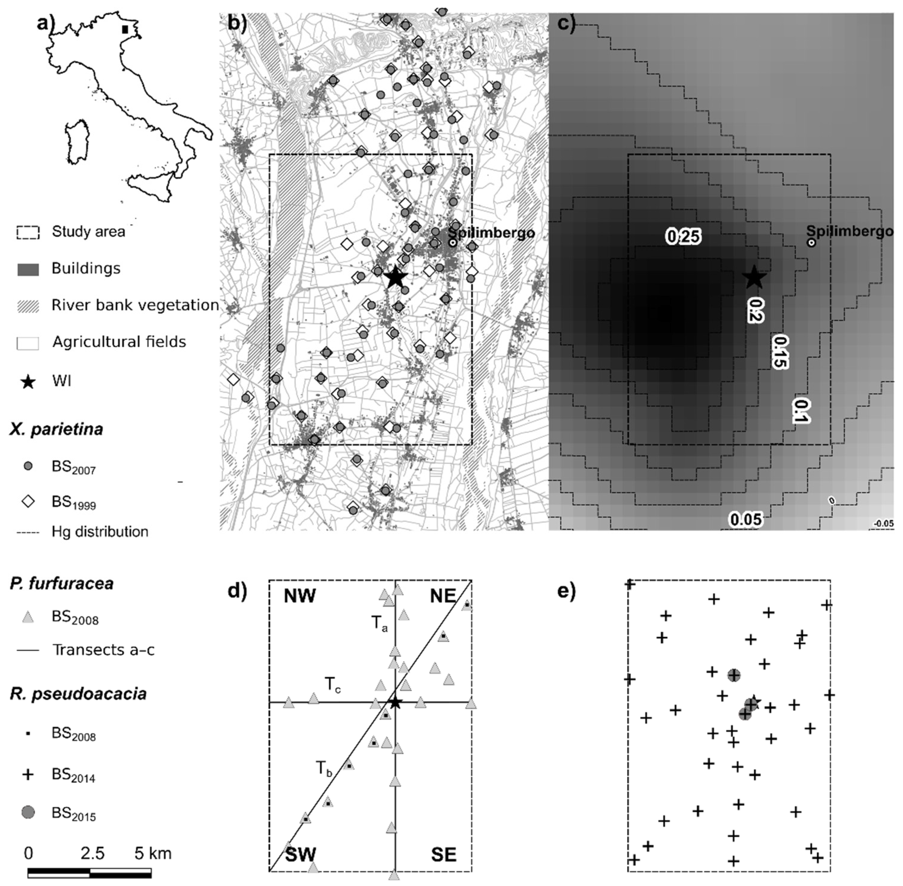
2.1. Study Area
2.2. Biomonitoring Surveys
2.3. Sample Treatments
2.3.1. Characterization of Robinia pseudoacacia Leaf Samples
2.4. Mercury Analysis
2.5. Data Analysis
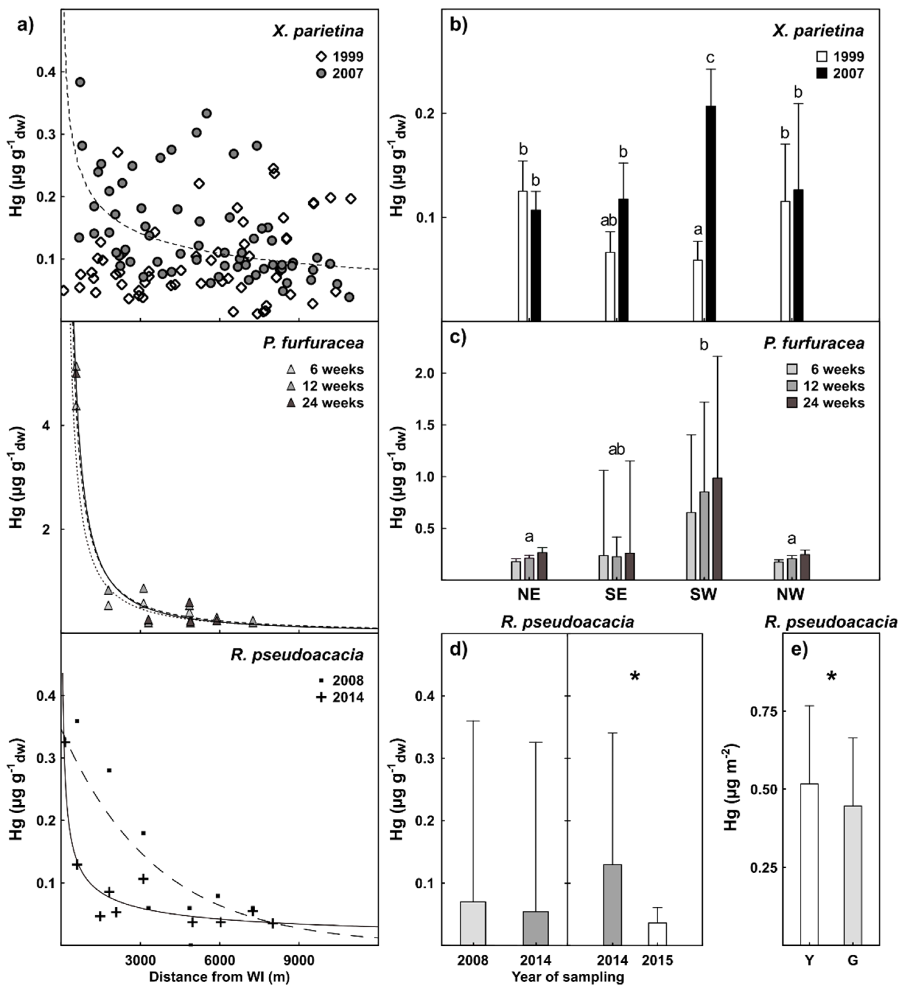
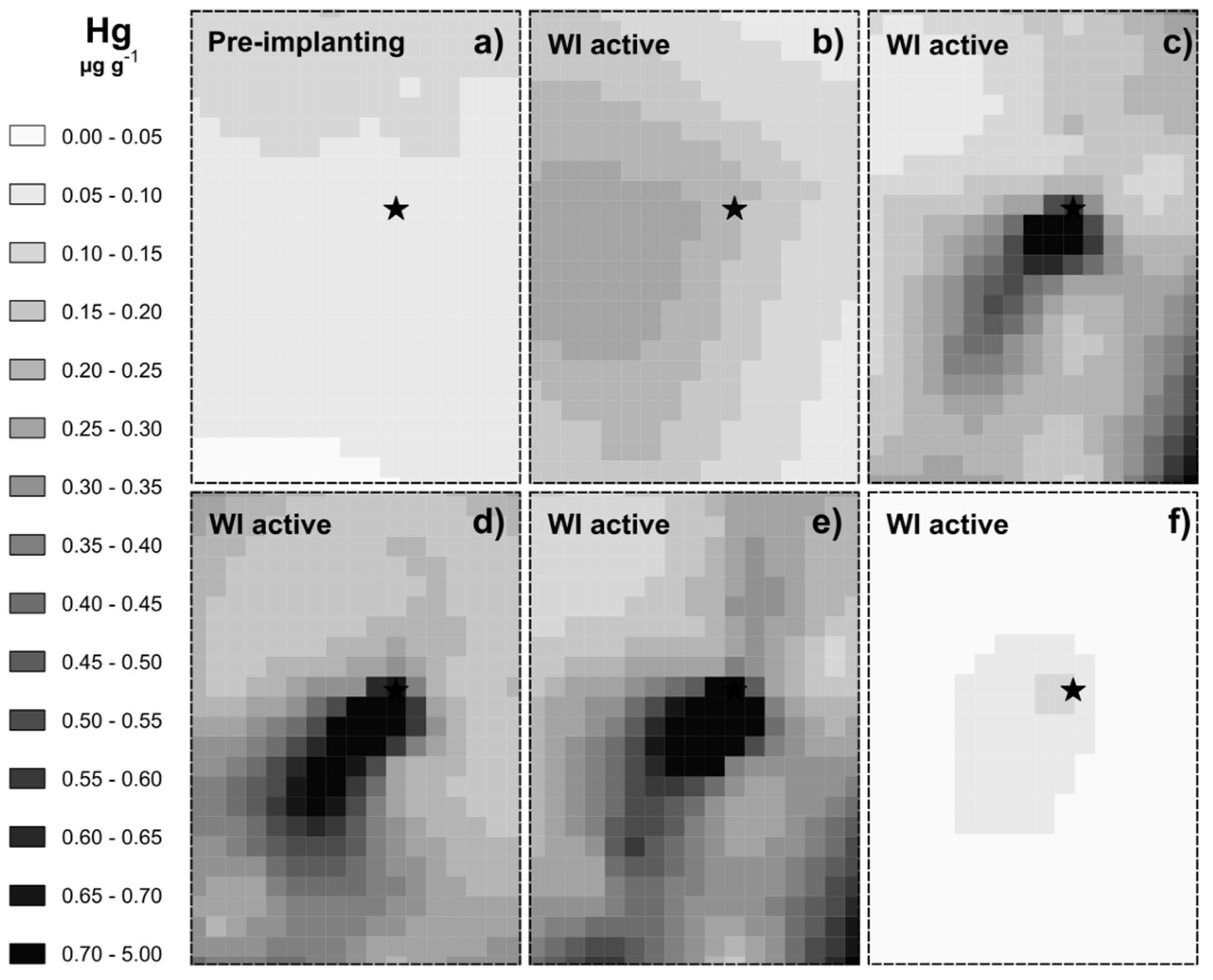
3. Results
4. Discussion
4.1. The Pattern of Hg Pollution
4.2. Comparison Among BSs’ Results
4.3. Effectiveness of Biomonitoring Techniques in Pollution and Monitoring Assessment Programs
5. Conclusions
Supplementary Materials
Author Contributions
Funding
Acknowledgments
Conflicts of Interest
References
- Selin, N.E. Global Biogeochemical Cycling of Mercury: A Review. Annu. Rev. Environ. Resour. 2009, 34, 43–63. [Google Scholar] [CrossRef]
- United Nations Environment Programme. UNEP Report of the Governing Council; Twenty-Fifth Session (16–20 February 2009), General Assembly, Supplement No. 25; United Nations Environment Programme: New York, NY, USA, 2009. [Google Scholar]
- Rafaj, P.; Bertok, I.; Cofala, J.; Schoepp, W. Scenarios of global mercury emissions from anthropogenic sources. Atmos. Environ. 2013, 79, 472–479. [Google Scholar] [CrossRef]
- European Parliament. Directive 2004/107/EC of the European Parliament and of the Council of 15 December 2004 relating to arsenic, cadmium, mercury, nickel and polycyclic aromatic hydrocarbons in ambient air. Off. J. Eur. Communities 2004, 23, 3–16. [Google Scholar]
- European Parliament. Directive 2008/50/EC of the European Parliament and of the Council of 21 May 2008 on ambient air quality and cleaner air for Europe. Off. J. Eur. Union 2008, 152, 1–44. [Google Scholar]
- European Parliament. Directive 2010/75/EU of the European Parliament and of the Council of 24 November 2010 on industrial emissions (integrated pollution prevention and control). Off. J. Eur. Union 2010, 334, 17–119. [Google Scholar]
- European Parliament. Regulation (EU) 2017/852 of the European Parliament and of the Council of 17 May 2017 on mercury, and repealing Regulation (EC) No 1102/2008. Off. J. Eur. Union 2017, 137, 1–21. [Google Scholar]
- Pirrone, N.; Aas, W.; Cinnirella, S.; Ebinghaus, R.; Hedgecock, I.M.; Pacyna, J.; Sprovieri, F.; Sunderland, E.M. Toward the next generation of air quality monitoring: Mercury. Atmos. Environ. 2013, 80, 599–611. [Google Scholar] [CrossRef]
- Sprovieri, F.; Pirrone, N.; Ebinghaus, R.; Kock, H.; Dommergue, A. A review of worldwide atmospheric mercury measurements. Atmos. Chem. Phys. Discuss. 2010, 10, 8245–8265. [Google Scholar] [CrossRef] [Green Version]
- Wolterbeek, H.T. Biomonitoring of trace element air pollution: Principles, possibilities and perspectives. Environ. Pollut. 2002, 120, 11–21. [Google Scholar] [CrossRef]
- Wolterbeek, H.T.; Garty, J.; Reis, M.A.; Freitas, M.C. Biomonitors in use: Lichens and metal air pollution. In Trace Metals and Other Contaminants in the Environment; Markert, B.A., Breure, A.M., Zechmeister, H.G., Eds.; Elsiever: Amsterdam, The Netherlands, 2006; Volume 6, pp. 377–419. [Google Scholar]
- Bargagli, R. Trace Elements in Terrestrial Plants an Ecophysiological Approach to Biomonitoring and Biorecovery; Springer: Berlin, Germany, 1998. [Google Scholar]
- Bargagli, R. Moss and lichen biomonitoring of atmospheric mercury: A review. Sci. Total Environ. 2016, 572, 216–231. [Google Scholar] [CrossRef]
- Tretiach, M.; Adamo, P.; Bargagli, R.; Baruffo, L.; Carletti, L.; Crisafulli, P.; Giordano, S.; Modenesi, P.; Orlando, S.; Pittao, E. Lichen and moss bags as monitoring devices in urban areas. Part I: Influence of exposure on sample vitality. Environ. Pollut. 2007, 146, 380–391. [Google Scholar] [CrossRef]
- Adamo, P.; Crisafulli, P.; Giordano, S.; Minganti, V.; Modenesi, P.; Monaci, F.; Pittao, E.; Tretiach, M.; Bargagli, R. Lichen and moss bags as monitoring devices in urban areas. Part II: Trace element content in living and dead biomonitors and comparison with synthetic materials. Environ. Pollut. 2007, 146, 392–399. [Google Scholar] [CrossRef]
- Giordano, S.; Adamo, P.; Monaci, F.; Pittao, E.; Tretiach, M.; Bargagli, R. Bags with oven-dried moss for the active monitoring of airborne trace elements in urban areas. Environ. Pollut. 2009, 157, 2798–2805. [Google Scholar] [CrossRef]
- De Nicola, F.; Spagnuolo, V.; Baldantoni, D.; Sessa, L.; Alfani, A.; Bargagli, R.; Monaci, F.; Terracciano, S.; Giordano, S. Improved biomonitoring of airborne contaminants by combined use of holm oak leaves and epiphytic moss. Chemosphere 2013, 92, 1224–1230. [Google Scholar] [CrossRef]
- Tretiach, M.; Candotto Carniel, F.; Loppi, S.; Carniel, A.; Bortolussi, A.; Mazzilis, D.; Del Bianco, C. Lichen transplants as a suitable tool to identify mercury pollution from waste incinerators: A case study from NE Italy. Environ. Monit. Assess. 2011, 175, 589–600. [Google Scholar] [CrossRef]
- Bargagli, R. Guidelines for the Use of Epiphytic Lichens as Biomonitors of Atmospheric Deposition of Trace Elements; Springer Nature: Basingstoke, UK, 2002; pp. 295–299. [Google Scholar]
- Petruzzellis, F.; Palandrani, C.; Savi, T.; Alberti, R.; Nardini, A.; Bacaro, G. Sampling intraspecific variability in leaf functional traits: Practical suggestions to maximize collected information. Ecol. Evol. 2017, 7, 11236–11245. [Google Scholar] [CrossRef] [PubMed] [Green Version]
- Tao, S. Kriging and mapping of copper, lead, and mercury contents in surface soil in Shenzhen area. Water Air Soil Pollut. 1995, 83, 161–172. [Google Scholar] [CrossRef]
- Heuvelink, G.B.; Pebesma, E.J. Is the ordinary kriging variance a proper measure of interpolation error. In Proceedings of the Fifth International Symposium on Spatial Accuracy Assessment in Natural Resources and Environmental Sciences, Melbourne, Australia, 10–12 July 2002; pp. 179–186. [Google Scholar]
- Gong, G.; Mattevada, S.; O’Bryant, S.E. Comparison of the accuracy of kriging and IDW interpolations in estimating groundwater arsenic concentrations in Texas. Environ. Res. 2014, 130, 59–69. [Google Scholar] [CrossRef]
- Fortuna, L.; Tretiach, M. Effects of site-specific climatic conditions on the radial growth of the lichen biomonitor Xanthoria parietina. Environ. Sci. Pollut. Res. 2018, 25, 34017–34026. [Google Scholar] [CrossRef]
- Keresztesi, B. Breeding and cultivation of black locust, Robinia pseudoacacia, in Hungary. For. Ecol. Manag. 1983, 6, 217–244. [Google Scholar] [CrossRef]
- Giordano, S.; Adamo, P.; Sorbo, S.; Vingiani, S. Atmospheric trace metal pollution in the Naples urban area based on results from moss and lichen bags. Environ. Pollut. 2005, 136, 431–442. [Google Scholar] [CrossRef] [PubMed]
- Petrova, S. Lichen-Bags as a Biomonitoring Technique in an Urban Area. Appl. Ecol. Environ. Res. 2015, 13, 915–923. [Google Scholar] [CrossRef]
- Protano, C.; Owczarek, M.; Antonucci, A.; Guidotti, M.; Vitali, M. Assessing indoor air quality of school environments: Transplanted lichen Pseudevernia furfuracea as a new tool for biomonitoring and bioaccumulation. Environ. Monit. Assess. 2017, 189, 358. [Google Scholar] [CrossRef] [PubMed]
- Cocozza, C.; Ravera, S.; Cherubini, P.; Lombardi, F.; Marchetti, M.; Tognetti, R. Integrated biomonitoring of airborne pollutants over space and time using tree rings, bark, leaves and epiphytic lichens. For. Green. 2016, 17, 177–191. [Google Scholar] [CrossRef]
- Pacyna, E.; Pacyna, J.; Sundseth, K.; Munthe, J.; Kindbom, K.; Wilson, S.; Steenhuisen, F.; Maxson, P. Global emission of mercury to the atmosphere from anthropogenic sources in 2005 and projections to 2020. Atmos. Environ. 2010, 44, 2487–2499. [Google Scholar]
- Costa, P.; Pacyna, J.; Pirrone, N.; Ferrara, R. Mercury emissions to the atmosphere from natural and anthropogenic sources in the Mediterranean region. Atmos. Environ. 2001, 35, 2997–3006. [Google Scholar]
- Cinnirella, S.; Finkelman, R.B.; Leaner, J.; Mukherjee, A.B.; Stracher, G.B.; Telmer, K.; Pirrone, N.; Feng, X.; Friedli, H.R.; Mason, R.; et al. Global mercury emissions to the atmosphere from anthropogenic and natural sources. Atmos. Chem. Phys. Discuss. 2010, 10, 5951–5964. [Google Scholar] [Green Version]
- Mukherjee, A.B.; Zevenhoven, R.; Brodersen, J.; Hylander, L.D.; Bhattacharya, P. Mercury in waste in the European Union: Sources, disposal methods and risks. Resour. Conserv. Recycl. 2004, 42, 155–182. [Google Scholar] [CrossRef]
- Canciani, L. Relazione Annuale Relative al Funzionamento ed alla Sorveglianza Dell’impianto di Coincenerimento e Termovalorizzazione di Rifiuti Speciali Pericolosi e non Pericolosi sito in zona Industriale del Cosa in Comune di Spilimbergo; Mistral FVG S.r.L: Spilimbergo, Italy, 2008. [Google Scholar]
- Cerovac, A.; Covelli, S.; Emili, A.; Pavoni, E.; Petranich, E.; Gregorič, A.; Urbanc, J.; Zavagno, E.; Zini, L. Mercury in the unconfined aquifer of the Isonzo/Soča River alluvial plain downstream from the Idrija mining area. Chemosphere 2018, 195, 749–761. [Google Scholar]
- Tretiach, M.; Pittao, E. Biomonitoraggio di Metalli Mediante Licheni in Cinque aree Campione della Provincia di Pordenone. Stato attuale e Confronto con i dati del 1999; Provincia di Pordenone: Pordenone, Italy, 2008. [Google Scholar]
- Nimis, P.L.; Bargagli, R. Linee-guida per l’utilizzo di licheni epifiti come bioaccumulatori di metalli in traccia. In Proceedings of the Atti del Workshop Biomonitoraggio della qualità dell’aria sul territorio nazionale, Roma, Italy, 26–27 November 1998; pp. 279–289. [Google Scholar]
- Scerbo, R.; Possenti, L.; Lampugnani, L.; Ristori, T.; Barale, R.; Barghigiani, C. Lichen (Xanthoria parietina) biomonitoring of trace element contamination and air quality assessment in Livorno Province (Tuscany, Italy). Sci. Total Environ. 1999, 241, 91–106. [Google Scholar] [CrossRef]
- Scerbo, R.; Ristori, T.; Possenti, L.; Lampugnani, L.; Barale, R.; Barghigiani, C. Lichen (Xanthoria parietina) biomonitoring of trace element contamination and air quality assessment in Pisa Province (Tuscany, Italy). Sci. Total Environ. 2002, 286, 27–40. [Google Scholar] [CrossRef]
- Cuny, D.; Davranche, L.; Thomas, P.; Kempa, M.; Van Haluwyn, C.; Haluwyn, C. Spatial and Temporal Variations of Trace Element Contents in Xanthoria Parietina Thalli Collected in a Highly Industrialized Area in Northern France as an Element for a Future Epidemiological Study. J. Atmos. Chem. 2004, 49, 391–401. [Google Scholar] [CrossRef]
- Demiray, A.D.; Yolcubal, I.; Akyol, N.H.; Çobanoğlu, G. Biomonitoring of airborne metals using the lichen Xanthoria parietina in Kocaeli Province, Turkey. Ecol. Indic. 2012, 18, 632–643. [Google Scholar] [CrossRef]
- Bargagli, R.; Barghigiani, C.; Siegel, B.; Siegel, S. Accumulation of mercury and other metals by the lichen, Parmelia sulcata, at an italian minesite and a volcanic area. Water Air Soil Pollut. 1989, 45, 315–327. [Google Scholar] [CrossRef]
- Loppi, S.; Paoli, L.; Gaggi, C. Diversity of epiphytic lichens and Hg contents of Xanthoria parietina thalli as monitors of geothermal air pollution in the Mt. Amiata area (central Italy). J. Atmos. Chem. 2006, 53, 93–105. [Google Scholar] [CrossRef]
- Ferretti, M.; Brambilla, E.; Brunialti, G.; Fornasier, F.; Mazzali, C.; Giordani, P.; Nimis, P. Reliability of different sampling densities for estimating and mapping lichen diversity in biomonitoring studies. Environ. Pollut. 2004, 127, 249–256. [Google Scholar] [CrossRef]
- Aboal, J.R.; Real, C.; Fernández, J.A.; Carballeira, A. Mapping the results of extensive surveys: The case of atmospheric biomonitoring and terrestrial mosses. Sci. Total Environ. 2006, 356, 256–274. [Google Scholar] [CrossRef] [PubMed]
- Real, C.; Aboal, J.; Fernandez, J.A.; Carballeira, A.; Aboal, J. The use of native mosses to monitor fluorine levels—And associated temporal variations—In the vicinity of an aluminium smelter. Atmos. Environ. 2003, 37, 3091–3102. [Google Scholar] [CrossRef]
- Hanson, P.J.; Lindberg, S.E.; Tabberer, T.A.; Owens, J.G.; Kim, K.-H. Foliar Exchange of Mercury Vapor: Evidence for a Compensation Point. Water Air Soil Pollut. 1995, 80, 373–382. [Google Scholar] [CrossRef]
- Millhollen, A.G.; Gustin, M.S.; Obrist, D. Foliar Mercury Accumulation and Exchange for Three Tree Species. Environ. Sci. Technol. 2006, 40, 6001–6006. [Google Scholar] [CrossRef] [PubMed]
- Walther, D.A.; Ramelow, G.J.; Beck, J.N.; Young, J.C.; Callahan, J.D.; Maroon, M.F. Temporal changes in metal levels of the lichens Parmotrema praesorediosum and Ramalina stenospora, southwest Louisiana. Water Air Soil Pollut. 1990, 53, 189–200. [Google Scholar] [CrossRef]
- Barghigiani, C.; Bargagli, R.; Siegel, B.; Siegel, S. Source and selectivity in the accumulation of mercury and other metals by the plants of Mt. Etna. Water Air Soil Pollut. 1988, 39, 395–408. [Google Scholar]
- Vannini, A.; Nicolardi, V.; Bargagli, R.; Loppi, S. Estimating Atmospheric Mercury Concentrations with Lichens. Environ. Sci. Technol. 2014, 48, 8754–8759. [Google Scholar] [CrossRef] [PubMed]
- Tretiach, M.; Crisafulli, P.; Pittao, E.; Rinino, S.; Roccotiello, E.; Modenesi, P. Isidia ontogeny and its effect on the CO2 gas exchanges of the epiphytic lichen Pseudevernia furfuracea (L.) Zopf. Lichenologist 2005, 37, 445–462. [Google Scholar] [CrossRef]
- Honegger, R. Developmental biology of lichens. New Phytol. 1993, 125, 659–677. [Google Scholar] [CrossRef] [Green Version]
- Rea, A.W.; Lindberg, S.E.; Scherbatskoy, T.; Keeler, G.J. Mercury Accumulation in Foliage over Time in Two Northern Mixed-Hardwood Forests. Water Air Soil Pollut. 2002, 133, 49–67. [Google Scholar] [CrossRef]
- Lindroth, R.; Osier, T.; Barnhill, H.; Wood, S. Effects of genotype and nutrient availability on phytochemistry of trembling aspen (Populus tremuloides Michx.) during leaf senescence. Biochem. Syst. Ecol. 2002, 30, 297–307. [Google Scholar] [CrossRef]
- Aboal, J.; Fernandez, J.A.; Boquete, T.; Carballeira, A.; Aboal, J.; Boquete, M.T. Is it possible to estimate atmospheric deposition of heavy metals by analysis of terrestrial mosses? Sci. Total Environ. 2010, 408, 6291–6297. [Google Scholar] [CrossRef] [PubMed]
- Schröder, W.; Holy, M.; Pesch, R.; Harmens, H.; Ilyin, I.; Steinnes, E.; Alber, R.; Aleksiayenak, Y.; Blum, O.; Coşkun, M.; et al. Are cadmium, lead and mercury concentrations in mosses across Europe primarily determined by atmospheric deposition of these metals? J. Soils Sediments 2010, 10, 1572–1584. [Google Scholar] [CrossRef]
- Incerti, G.; Cecconi, E.; Capozzi, F.; Adamo, P.; Bargagli, R.; Benesperi, R.; Carniel, F.C.; Cristofolini, F.; Giordano, S.; Puntillo, D.; et al. Infraspecific variability in baseline element composition of the epiphytic lichen Pseudevernia furfuracea in remote areas: Implications for biomonitoring of air pollution. Environ. Sci. Pollut. Res. 2017, 24, 8004–8016. [Google Scholar] [CrossRef]
- Cecconi, E.; Incerti, G.; Capozzi, F.; Adamo, P.; Bargagli, R.; Benesperi, R.; Carniel, F.C.; Favero-Longo, S.E.; Giordano, S.; Puntillo, D.; et al. Background element content of the lichen Pseudevernia furfuracea: A supra-national state of art implemented by novel field data from Italy. Sci. Total Environ. 2018, 622, 282–292. [Google Scholar] [CrossRef] [PubMed]
- Cecconi, E.; Fortuna, L.; Benesperi, R.; Bianchi, E.; Brunialti, G.; Contardo, T.; Di Nuzzo, L.; Frati, L.; Monaci, F.; Munzi, S.; et al. New Interpretative Scales for Lichen Bioaccumulation Data: The Italian Proposal. Atmosphere 2019, 10, 136. [Google Scholar] [CrossRef]
- Frati, L.; Brunialti, G.; Loppi, S. Problems Related to Lichen Transplants to Monitor Trace Element Deposition in Repeated Surveys: A Case Study from Central Italy. J. Atmos. Chem. 2005, 52, 221–230. [Google Scholar] [CrossRef]


| Series of Samples | Technique | Year | Biomonitor |
|---|---|---|---|
| Xp1999 | P | 1999 | X. parietina, native |
| Xp2007 | P | 2007 | X. parietina, native |
| Pf-62008 | A | 2008 | P. furfuracea, transplants |
| Pf-122008 | A | 2008 | P. furfuracea, transplants |
| Pf-242008 | A | 2008 | P. furfuracea, transplants |
| Rp2008 | P | 2008 | Green leaves of R. pseudoacacia, native |
| Rp-G2014 | P | 2014 | Green leaves of R. pseudoacacia, native |
| Rp-Y2014 | P | 2014 | Yellow leaves of R. pseudoacacia, native |
| Rp2015 | P | 2015 | Green leaves of R. pseudoacacia, native |
| Parameters | X. parietina | P. furfuracea | R. pseudoacacia | ||||||
|---|---|---|---|---|---|---|---|---|---|
| WI status | off | on | on | on | on | off | |||
| BS | BS1999 | BS2007 | BS2008 | BS2008 | BS2014 | BS2015 | |||
| Sample Series | Xp1999 | Xp2007 | Pf-62008 | Pf-122008 | Pf-242008 | Rp2008 | Rp-G2014 | Rp-Y2014 | Rp2015 |
| Exposure Period (Weeks) | ~52 | ~52 | 6 | 12 | 24 | ~40 | ~40 | ~40 | ~40 |
| n | 56 | 64 | 30 | 30 | 30 | 8 | 39 | 8 | 3 |
| Min | 0.011 | 0.039 | 0.130 | 0.150 | 0.130 | 0.000 | 0.017 | 0.024 | 0.023 |
| Max | 0.270 | 0.384 | 4.370 | 5.130 | 5.000 | 0.360 | 0.326 | 0.425 | 0.061 |
| Mean | 0.096 | 0.141 | 0.371 | 0.467 | 0.500 | 0.135 | 0.052 | 0.106 | 0.040 |
| St. dev. | 0.064 | 0.078 | 0.764 | 0.899 | 0.919 | 0.126 | 0.052 | 0.135 | 0.019 |
| CV% | 66.6 | 55.5 | 206.0 | 192.5 | 183.9 | 93.6 | 101.0 | 126.7 | 47.4 |
| SS | MS | F | p | |
|---|---|---|---|---|
| X. parietina | ||||
| Intercept | 0.50 | 0.50 | 136.64 | <0.001 |
| Distance (D) | 0.02 | 0.02 | 5.93 | 0.016 |
| Year (Y) | 0.05 | 0.05 | 13.01 | <0.001 |
| Wind (W) | 0.02 | 0.01 | 2.15 | 0.098 |
| Y × W | 0.16 | 0.05 | 14.23 | <0.001 |
| Error | 0.41 | 0.00 | ||
| Total | 0.67 | |||
| Model | 0.26 | 0.03 | 8.72 | <0.001 |
| P. furfuracea | ||||
| Intercept | 18.21 | 18.21 | 30.50 | <0.001 |
| D | 10.40 | 10.40 | 17.41 | <0.001 |
| Exposure (E) | 0.16 | 0.08 | 0.13 | 0.877 |
| W | 13.37 | 4.46 | 7.46 | <0.001 |
| E × W | 0.23 | 0.04 | 0.06 | 0.998 |
| Error | 44.19 | 0.60 | ||
| Total | 62.60 | |||
| Model | 18.41 | 1.53 | 2.57 | <0.001 |
| Set of Samples | RMSE | Variance Range | Xp1999 | Xp2007 | Pf-62008 | Pf-122008 | Pf-242008 | Rp-G2014 |
|---|---|---|---|---|---|---|---|---|
| Xp1999 | 0.0315 | ≃0 | 1 | |||||
| Xp2007 | 0.0345 | [0.002, 0.003] | −0.054 | 1 | ||||
| Pf-62008 | 0.3375 | [0.029, 0.247] | −0.220 | 0.023 | 1 | |||
| Pf-122008 | 0.0892 | [−0.124, 0.122] | −0.218 | 0.327 | 0.90 | 1 | ||
| Pf-242008 | 0.334 | [−0.176, 0.663] | −0.271 | 0.121 | 0.970 | 0.934 | 1 | |
| Rp-G2014 | 0.0093 | [0.017, 0.152] | −0.341 | 0.546 | 0.546 | 0.662 | 0.616 | 1 |
© 2019 by the authors. Licensee MDPI, Basel, Switzerland. This article is an open access article distributed under the terms and conditions of the Creative Commons Attribution (CC BY) license (http://creativecommons.org/licenses/by/4.0/).
Share and Cite
Fortuna, L.; Candotto Carniel, F.; Capozzi, F.; Tretiach, M. Congruence Evaluation of Mercury Pollution Patterns Around a Waste Incinerator over a 16-Year-Long Period Using Different Biomonitors. Atmosphere 2019, 10, 183. https://doi.org/10.3390/atmos10040183
Fortuna L, Candotto Carniel F, Capozzi F, Tretiach M. Congruence Evaluation of Mercury Pollution Patterns Around a Waste Incinerator over a 16-Year-Long Period Using Different Biomonitors. Atmosphere. 2019; 10(4):183. https://doi.org/10.3390/atmos10040183
Chicago/Turabian StyleFortuna, Lorenzo, Fabio Candotto Carniel, Fiore Capozzi, and Mauro Tretiach. 2019. "Congruence Evaluation of Mercury Pollution Patterns Around a Waste Incinerator over a 16-Year-Long Period Using Different Biomonitors" Atmosphere 10, no. 4: 183. https://doi.org/10.3390/atmos10040183
APA StyleFortuna, L., Candotto Carniel, F., Capozzi, F., & Tretiach, M. (2019). Congruence Evaluation of Mercury Pollution Patterns Around a Waste Incinerator over a 16-Year-Long Period Using Different Biomonitors. Atmosphere, 10(4), 183. https://doi.org/10.3390/atmos10040183