The Impact of Meteorological and Hydrological Memory on Compound Peak Flows in the Rhine River Basin

 ,
,  , and
, and
Abstract
1. Introduction
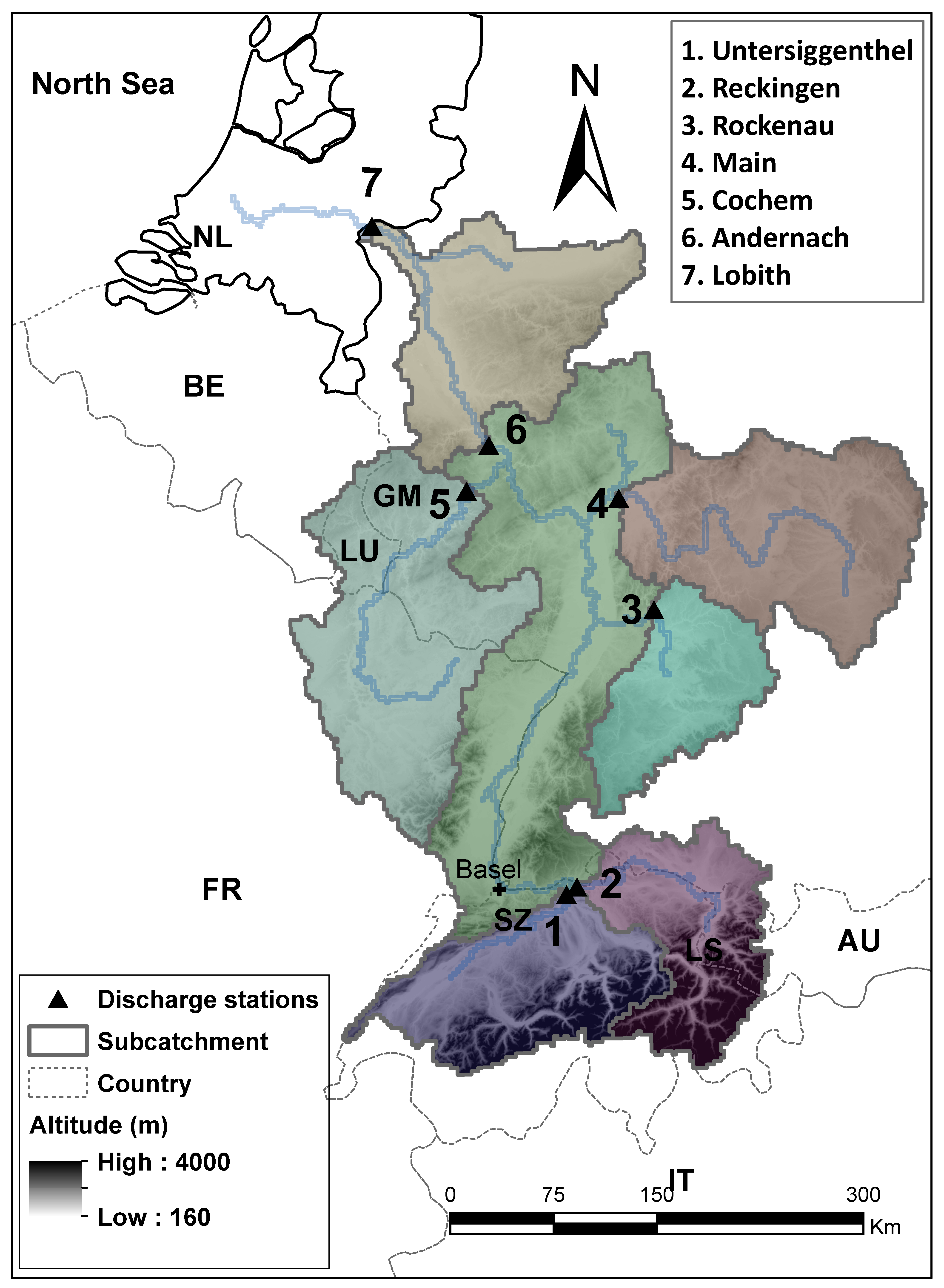
2. Study Area
3. Data, Model and Methods
3.1. Data
3.2. Hydrological Model
3.3. Snow Memory Effects
3.4. Soil Moisture Memory Effects
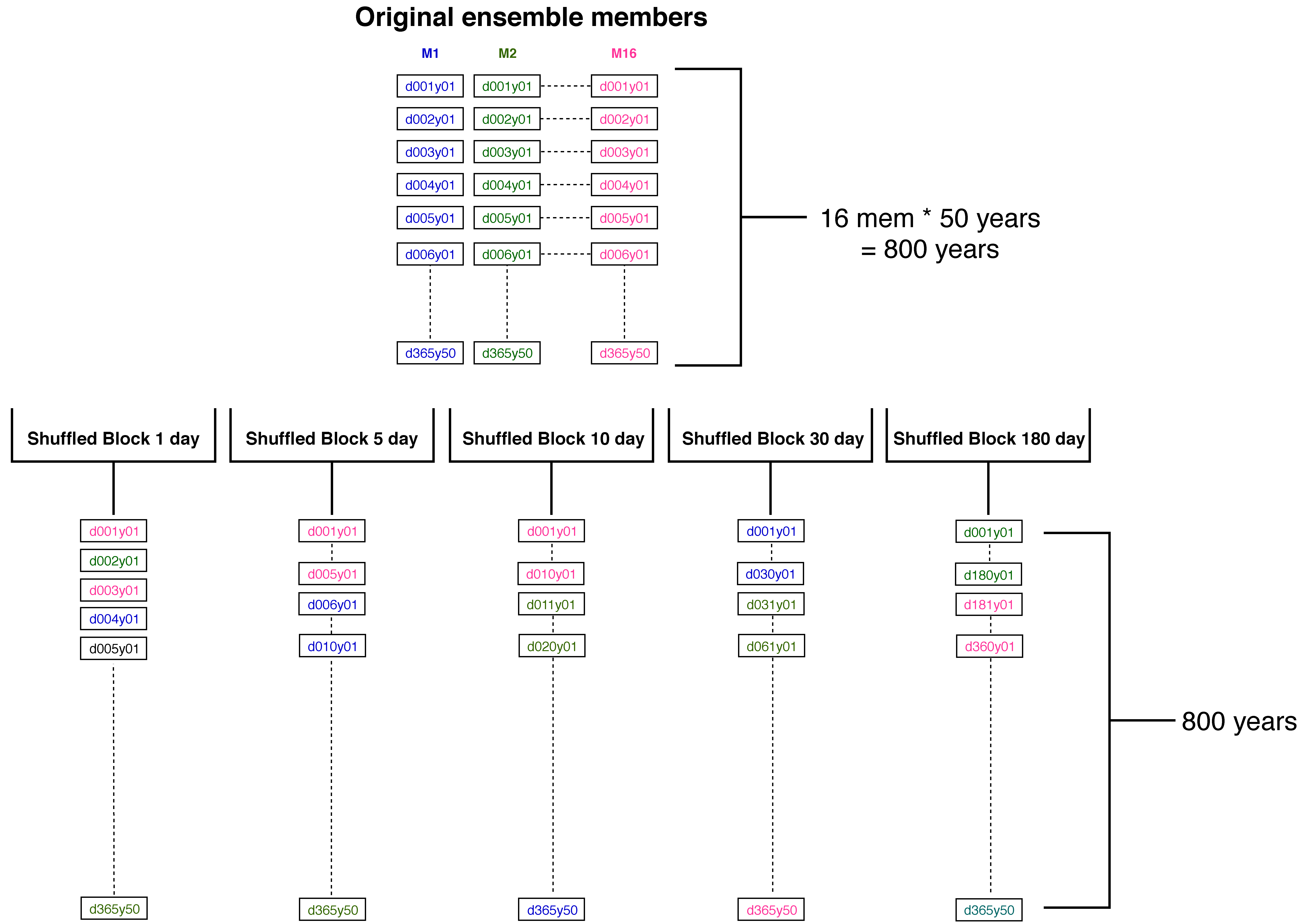
3.5. Meteorological Autocorrelation
4. Results and Discussion
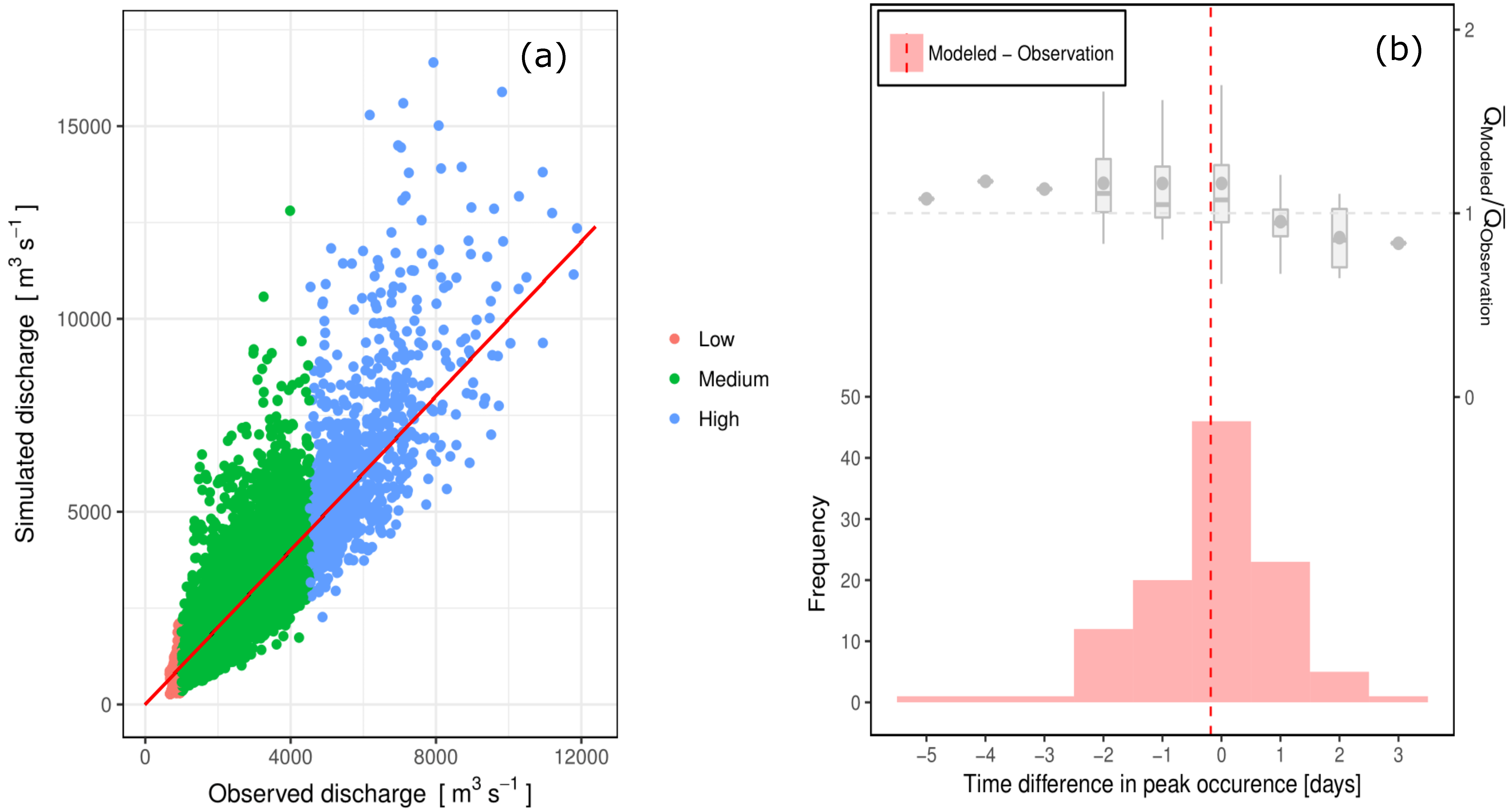
4.1. Performance of the Hydrological Model
4.1.1. Daily Flows
4.1.2. Flood Wave Timings
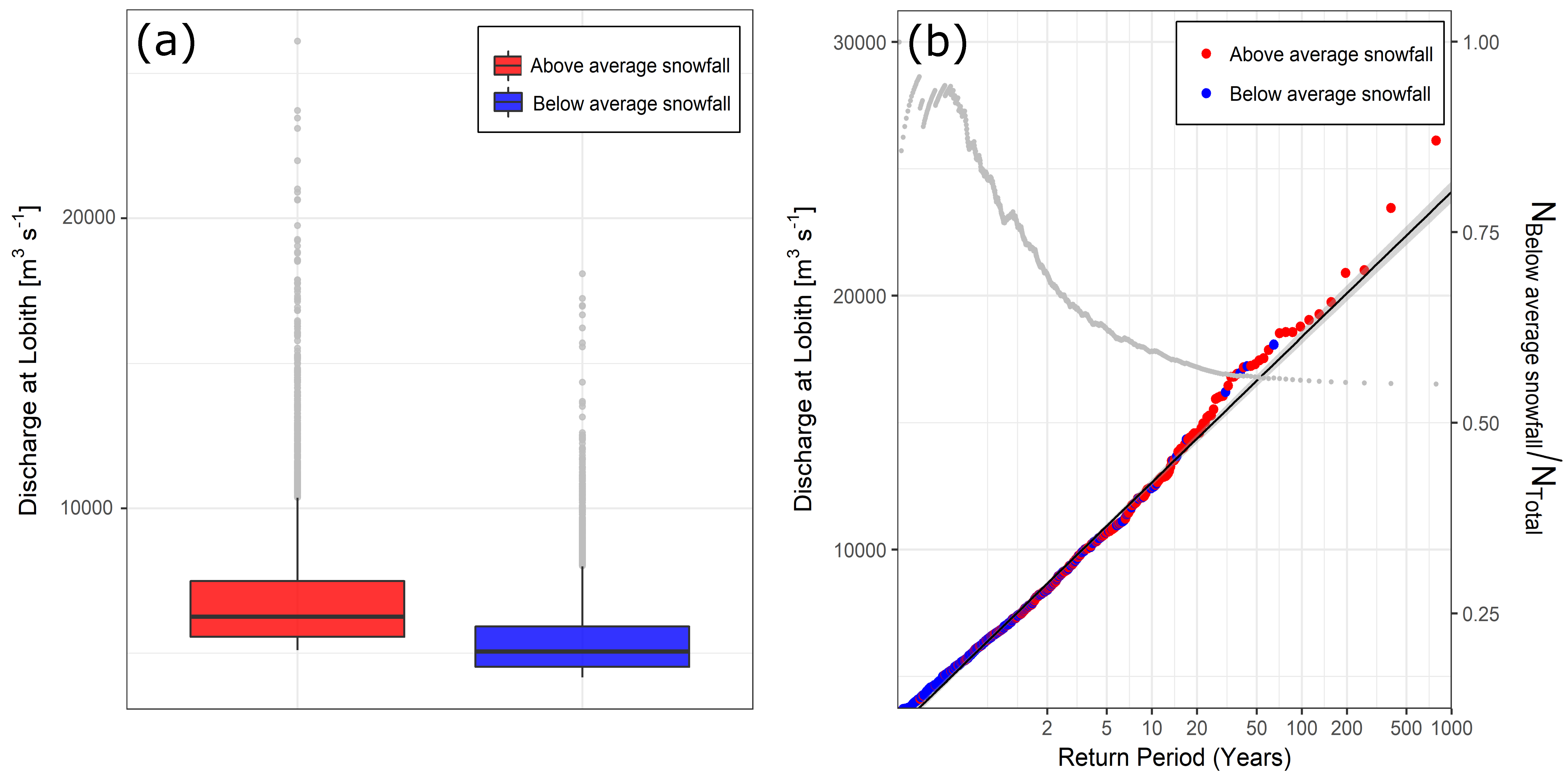
4.2. Snow Memory Effects
4.3. Soil Moisture Memory Effects
4.4. Meteorological Autocorrelation
4.4.1. Importance of Autocorrelation
4.4.2. Case Studies
5. Discussion and Conclusions
Supplementary Materials
Author Contributions
Funding
Acknowledgments
Data availability
Conflicts of Interest
References
- Wu, W.; Dickinson, R.E. Time scales of layered soil moisture memory in the context of land-atmosphere interaction. J. Clim. 2004, 17, 2752–2764. [Google Scholar] [CrossRef]
- Vinnikov, K.Y.; Robock, A.; Speranskaya, N.A.; Schlosser, C.A. Scales of temporal and spatial variability of mitlatitude soil moisture. J. Geophys. Res. 1996, 101, 7163–7174. [Google Scholar] [CrossRef]
- Entin, J.K.; Robock, A.; Vinnikov, K.Y.; Hollinger, S.E.; Liu, S.; Namkhai, A. Meteorologic i Land Surface. J. Geophys. Res. 2000, 105, 11865–11877. [Google Scholar] [CrossRef]
- Lorenz, E.N. The predictability of a flow which possesses many scales of motion. Tellus 1969, 21, 289–307. [Google Scholar] [CrossRef]
- Pelletier, J.D.; Turcotte, D.L. Long-range persistence in climatological and hydrological time series: Analysis, modeling and application to drought hazard assessment. J. Hydrol. 1997, 203, 198–208. [Google Scholar] [CrossRef]
- Wanders, N.; Thober, S.; Kumar, R.; Pan, M.; Sheffield, J.; Samaniego, L.; Wood, E.F. Development and evaluation of a Pan-European multi-model seasonal hydrological forecasting system. J. Hydrometeorol. 2019, 20, 99–115. [Google Scholar] [CrossRef]
- Koutsoyiannis, D. Hydrologic Persistence and The Hurst Phenomenon. Water Encycl. 2005. [Google Scholar] [CrossRef]
- Delworth, T.L.; Manabe, S. The Influence of Potential Evaporation on the Variabilities of Simulated Soil Wetness and Climate. J. Clim. 1988, 1, 523–547. [Google Scholar] [CrossRef]
- Scott, R.; Entekhabi, D.; Koster, R.; Suarez, M. Timescales of land surface evapotranspiration response. J. Clim. 1997, 10, 559–566. [Google Scholar] [CrossRef]
- Amenu, G.G.; Kumar, P.; Liang, X.-Z. Interannual Variability of Deep-Layer Hydrologic Memory and Mechanisms of Its Influence on Surface Energy Fluxes. J. Clim. 2005, 18, 5024–5045. [Google Scholar] [CrossRef]
- Güntner, A.; Stuck, J.; Werth, S.; Döll, P.; Verzano, K.; Merz, B. A global analysis of temporal and spatial variations in continental water storage. Water Resour. Res. 2007, 43, 1–19. [Google Scholar] [CrossRef]
- Seneviratne, S.I.; Koster, R.D. A Revised Framework for Analyzing Soil Moisture Memory in Climate Data: Derivation and Interpretation. J. Hydrometeorol. 2012, 13, 404–412. [Google Scholar] [CrossRef]
- Bojariu, R.; Gimeno, L. The role of snow cover fluctuations in multiannual NAO persistence. Geophys. Res. Lett. 2003, 30, 1–4. [Google Scholar] [CrossRef]
- Cohen, J.; Fletcher, C. Improved skill of northern hemisphere winter surface temperature predictions based on land-atmosphere fall anomalies. J. Clim. 2007, 20, 4118–4132. [Google Scholar] [CrossRef]
- Xu, L.; Dirmeyer, P. Snow-atmosphere coupling strength in a global atmospheric model. Geophys. Res. Lett. 2011, 38. [Google Scholar] [CrossRef]
- Hurst, H.E. Long-term storage capacity of reservoirs. Trans. Am. Soc. Civ. Eng. 1951, 116, 770–808. [Google Scholar]
- Montanari, A.; Rosso, R.; Taqqu, M.S. Fractionally dilferenced ARIMA models applied to hydrologic time series: Identification, estimation, and simulation. Water Resour. Res 1997, 33, 1035–1044. [Google Scholar] [CrossRef]
- Koutsoyiannis, D. The Hurst phenomenon and fractional Gaussian noise made easy The Hurst phenomenon and fractional Gaussian noise made easy. Hydrol. Sci. J. 2002, 47, 573–595. [Google Scholar] [CrossRef]
- Blender, R.; Fraedrich, K. Long-term memory of the hydrological cycle and river runoffs in China in a high-resolution climate model. Int. J. Climatol. 2006, 26, 1547–1565. [Google Scholar] [CrossRef]
- Mudelsee, M.; Borngen, M.; Tetzlaff, G.; Grunewald, U. No Upward Trends İn The Occurrence Of Extreme Floods İn Central Europe. Nature 2003, 425, 166–169. [Google Scholar] [CrossRef]
- Bunde, A.; Eichner, J.F.; Kantelhardt, J.W.; Havlin, S. Long-term memory: A natural mechanism for the clustering of extreme events and anomalous residual times in climate records. Phys. Rev. Lett. 2005, 94, 1–4. [Google Scholar] [CrossRef] [PubMed]
- Koster, R.D.; Suarez, M.J. Soil Moisture Memory in Climate Models. J. Hydrometeorol. 2001, 2, 558–570. [Google Scholar] [CrossRef]
- Orth, R.; Seneviratne, S.I. Analysis of soil moisture memory from observations in Europe. J. Geophys. Res. Atmos. 2012, 117, 1–19. [Google Scholar] [CrossRef]
- Dirmeyer, P.A.; Schlosser, C.A.; Brubaker, K.L. Precipitation, Recycling, and Land Memory: An Integrated Analysis. J. Hydrometeorol. 2009, 10, 278–288. [Google Scholar] [CrossRef]
- Bierkens, M.F.P.; van den Hurk, B.J.J.M. Groundwater convergence as a possible mechanism for multi-year persistence in rainfall. Geophys. Res. Lett. 2007, 34, 1–5. [Google Scholar] [CrossRef]
- Van Lanen, H.A.J.; Wanders, N.; Tallaksen, L.M.; Van Loon, A.F. Hydrological drought across the world: Impact of climate and physical catchment structure. Hydrol. Earth Syst. Sci. 2013, 17, 1715–1732. [Google Scholar] [CrossRef]
- Shinoda, M. Climate memory of snow mass as soil moisture over central Eurasia. J. Geophys. Res. Atmos. 2001, 106, 33393–33403. [Google Scholar] [CrossRef]
- Cohen, J.; Rind, D. The Effect of Snow Cover on the Climate. J. Clim. 1991, 4, 689–706. [Google Scholar] [CrossRef]
- Zscheischler, J.; Westra, S.; Van Den Hurk, B.J.J.M.; Seneviratne, S.I.; Ward, P.J.; Pitman, A.; Aghakouchak, A.; Bresch, D.N.; Leonard, M.; Wahl, T.; et al. Future climate risk from compound events. Nat. Clim. Chang. 2018, 8, 469–477. [Google Scholar] [CrossRef]
- Nicholson, S.E. Land Surface Processes and Land Use Change Land. Rev. Geophys. 2000, 38, 117–139. [Google Scholar] [CrossRef]
- Bonan, G.B.; Stillwell-soller, L.M. Soil water and the persistence of floods and droughts in the Mississippi River Basin. Water Resour. Res. 1998, 34, 2693–2701. [Google Scholar] [CrossRef]
- Liu, D.; Wang, G.; Mei, R.; Yu, Z.; Yu, M. Impact of initial soil moisture anomalies on climate mean and extremes over Asia. J. Geophys. Res. 2014, 119, 529–545. [Google Scholar] [CrossRef]
- van den Hurk, B.; van Meijgaard, E.; de Valk, P.; van Heeringen, K.-J.; Gooijer, J. Analysis of a compounding surge and precipitation event in the Netherlands. Environ. Res. Lett. 2015, 10, 035001. [Google Scholar] [CrossRef]
- Kew, S.F.; Selten, F.M.; Lenderink, G.; Hazeleger, W. The simultaneous occurrence of surge and discharge extremes for the Rhine delta. Nat. Hazards Earth Syst. Sci. 2013, 13, 2017–2029. [Google Scholar] [CrossRef]
- Khanal, S.; Ridder, N.; de Vries, H.; Terink, W.; van den Hurk, B. Storm surge and extreme river discharge: A compound event analysis using ensemble impact modelling. Hydrol. Earth Syst. Sci. Discuss. 2018. [Google Scholar] [CrossRef]
- Leonard, M.; Westra, S.; Phatak, A.; Lambert, M.; van den Hurk, B.; Mcinnes, K.; Risbey, J.; Schuster, S.; Jakob, D.; Stafford-Smith, M. A compound event framework for understanding extreme impacts. Wiley Interdiscip. Rev. Clim. Chang. 2014, 5, 113–128. [Google Scholar] [CrossRef]
- Wahl, T.; Haigh, I.D.; Nicholls, R.J.; Arns, A.; Dangendorf, S.; Hinkel, J.; Slangen, A.B.A. Understanding extreme sea levels for broad-scale coastal impact and adaptation analysis. Nat. Commun. 2017, 8, 16075. [Google Scholar] [CrossRef] [PubMed]
- Hazeleger, W.; van den Hurk, B.J.J.M.; Min, E.; van Oldenborgh, G.J.; Petersen, A.C.; Stainforth, D.A.; Vasileiadou, E.; Smith, L.A. Tales of future weather. Nat. Clim. Chang. 2015, 5, 107–113. [Google Scholar] [CrossRef]
- Seneviratne, S.; Nicholls, N.; Easterling, D.; Goodess, C.; Kanae, S.; Kossin, J.; Luo, Y.; Marengo, J.; McInnes, K.; Rahimi, M.; et al. Changes in climate extremes and their impacts on the natural physical environment. Manag. Risk Extrem. Events Disasters to Adv. Clim. Chang. Adapt. 2012, 109–230. [Google Scholar]
- Ridder, N.; de Vries, H.; Drijfhout, S. The Role of Atmospheric Rivers in compound events consisting of heavy precipitation and high storm surges along the Dutch coast. Nat. Hazards Earth Syst. Sci. Discuss. 2018, 18, 3311–3326. [Google Scholar] [CrossRef]
- Klerk, W.J.; Winsemius, H.C.; van Verseveld, W.J.; Bakker, A.M.R.; Diermanse, F.L.M. The co-incidence of storm surges and extreme discharges within the Rhine–Meuse Delta. Environ. Res. Lett. 2015, 10, 035005. [Google Scholar] [CrossRef]
- Pinter, N.; Van der Ploeg, R.R.; Schweigert, P.; Hoefer, G. Flood magnification on the River Rhine. Hydrol. Process. 2006, 20, 147–164. [Google Scholar] [CrossRef]
- Te Linde, A.H.; Aerts, J.C.J.H.; Bakker, A.M.R.; Kwadijk, J.C.J. Simulating low-probability peak discharges for the Rhine basin using resampled climate modeling data. Water Resour. Res. 2010, 46, 1–19. [Google Scholar] [CrossRef]
- Junghans, N.; Cullmann, J.; Huss, M. Evaluating the effect of snow and ice melt in an Alpine headwater catchment and further downstream in the River Rhine. Hydrol. Sci. J. 2011, 56, 981–993. [Google Scholar] [CrossRef]
- Stahl, K.; Weiler, M.; Kohn, I.; Freudiger, D.; Seibert, J.; Vis, M.; Gerlinger, K. The snow and glacier melt components of streamflow of the river Rhine and its tributaries considering the influence of climate change. Available online: https://www.chr-khr.org/en/publication/snow-and-glacier-melt-components-streamflow-river-rhine-and-its-tributaries-considerin-0 (accessed on 31 March 2019).
- Engel, H. The flood events of 1993/1994 and 1995 in the Rhine River basin. In Destructive Water: Water-Caused Natural Disasters, Their Abatement and Control; IAHS Publication No 239; Leavesly, G.H., Lins, H.F., Nobilis, F., Parker, R.S., Schneider, V.R., Van de Ven, F.H.M., Eds.; IAHS Press: Wallingford, UK, 1997; pp. 21–32. [Google Scholar]
- Disse, M.; Engel, H. Flood events in the Rhine basin: Genesis, influences and mitigation. Nat. Hazards 2001, 23, 271–290. [Google Scholar] [CrossRef]
- Kew, S.F.; Selten, F.M.; Lenderink, G.; Hazeleger, W. Robust assessment of future changes in extreme precipitation over the Rhine basin using a GCM. Hydrol. Earth Syst. Sci. 2011, 15, 1157–1166. [Google Scholar] [CrossRef]
- Hegnauer, M.; Kwadijk, J.; Klijn, F. The Plausibility of Extreme High Discharges in the River Rhine; Deltares: Delft, The Netherlands, 2015. [Google Scholar]
- Minville, M.; Velázquez, J.A.; Gauvin St-Denis, B.; Muerth, M.J.; Schmid, J.; Chaumont, D.; Ludwig, R.; Caya, D.; Turcotte, R.; Ricard, S. On the need for bias correction in regional climate scenarios to assess climate change impacts on river runoff. Hydrol. Earth Syst. Sci. 2013, 17, 1189–1204. [Google Scholar]
- Brienen, S.; Rust, H.W.; Sauter, T.; Themeßl, M.; Venema, V.K.C.; Chun, K.P.; Maraun, D.; Wetterhall, F.; Ireson, A.M.; Chandler, R.E.; et al. Precipitation Downscaling Under Climate Change: Recent Developments To Bridge the Gap Between Dynamical Models and the End User. Rev. Geophys. 2010, 48, 1–34. [Google Scholar]
- Kleinn, J.; Frei, C.; Gurtz, J.; Lüthi, D.; Vidale, P.L.; Schär, C. Hydrologic simulations in the Rhine basin driven by a regional climate model. J. Geophys. Res. D Atmos. 2005, 110, 1–18. [Google Scholar] [CrossRef]
- Viviroli, D.; Messerli, B. Assessing the Hydrological Significance of the World’s Mountains. Mt. Res. Dev. 2003, 23, 369–375. [Google Scholar] [CrossRef]
- Photiadou, C.S.; Weerts, A.H.; Van Den Hurk, B.J.J.M. Evaluation of two precipitation data sets for the Rhine River using streamflow simulations. Hydrol. Earth Syst. Sci. 2011, 15, 3355–3366. [Google Scholar] [CrossRef]
- Kwadijk, J.; Van Deursen, W. Internationale Kommission für die Hydrologie des Rheingebietes Commission Internationale de l’Hydrologie du Bassin du Rhin Development and Testing of a GIS Based Water Balance Model for the Rhine Drainage Basin; Utrecht University: Utrecht, The Netherlands, 1999. [Google Scholar]
- Hegnauer, M.; Beersma, J.J.; van den Boogaard, H.F.P.; Buishand, T.A.; Passchier, R.H. Generator of Rainfall and Discharge Extremes (GRADE) for the Rhine and Meuse Basins; Final Report of GRADE 2.0; Deltares: Delft, The Netherlands, 2014. [Google Scholar]
- Ward, P.J.; Jongman, B.; Aerts, J.C.J.H.; Bates, P.D.; Botzen, W.J.W.; Diaz Loaiza, A.; Hallegatte, S.; Kind, J.M.; Kwadijk, J.; Scussolini, P.; et al. A global framework for future costs and benefits of river-flood protection in urban areas. Nat. Clim. Chang. 2017, 7, 642. [Google Scholar] [CrossRef]
- Hazeleger, W.; Wang, X.; Severijns, C.; Ştefǎnescu, S.; Bintanja, R.; Sterl, A.; Wyser, K.; Semmler, T.; Yang, S.; van den Hurk, B.; et al. EC-Earth V2.2: Description and validation of a new seamless earth system prediction model. Clim. Dyn. 2012, 39, 2611–2629. [Google Scholar] [CrossRef]
- van Meijgaard, E.; Ulft, L.H. Van; Bosveld, F.C.; Lenderink, G.; Siebesma, A.P. The KNMI Regional Atmospheric Climate Model RACMO Version 2.1; Technical Report, TR-302; The Royal Netherlands Meteorological Institute: De Bilt, Netherlands, 2008; p. 43. [Google Scholar]
- Haylock, M.R.; Hofstra, N.; Klein Tank, A.M.G.; Klok, E.J.; Jones, P.D.; New, M. A European daily high-resolution gridded data set of surface temperature and precipitation for 1950–2006. J. Geophys. Res. Atmos. 2008, 113. [Google Scholar] [CrossRef]
- Terink, W.; Lutz, A.F.; Simons, G.W.H.; Immerzeel, W.W.; Droogers, P. SPHY: Spatial Processes in Hydrology. Geosci. Model Dev. Discuss. 2015, 8, 1687–1748. [Google Scholar] [CrossRef]
- Hock, R. Temperature index melt modelling in mountain areas. J. Hydrol. 2003, 282, 104–115. [Google Scholar] [CrossRef]
- Hargreaves, G.H.; Samani, Z.A. Reference Crop Evapotranspiration from Temperature. Appl. Eng. Agric. 2013, 1, 96–99. [Google Scholar] [CrossRef]
- Sutanudjaja, E.H.; Van Beek, R.; Wanders, N.; Wada, Y.; Bosmans, J.H.C.; Drost, N.; Van Der Ent, R.J.; De Graaf, I.E.M.; Hoch, J.M.; De Jong, K.; et al. PCR-GLOBWB 2: A 5 arcmin global hydrological and water resources model. Geosci. Model Dev. 2018, 11, 2429–2453. [Google Scholar] [CrossRef]
- GRDC. Available online: http://www.bafg.de/GRDC/EN/01_GRDC/grdc_node.html (accessed on 1 November 2016).
- Rajagopalan, B.; Lall, U. A k-nearest-neighbor Simulator for Daily Precipitation and Other Variables. Water Resour. Res. 1999, 35, 3089–3101. [Google Scholar] [CrossRef]
- Beersma, J. Extreme Hydro-Meteorological Events and Their Probabilities; Wagenngen University: Wageningen, The Netherlands, 2007; ISBN 9085046157. [Google Scholar]
- Nash, J.E.; Sutcliffe, J.V. River Flow Forecasting Through Conceptual Models Part I-a Discussion of Principles. J. Hydrol. 1970, 10, 282–290. [Google Scholar] [CrossRef]
- Sivapalan, M.; Blöschl, G.; Merz, R.; Gutknecht, D. Linking flood frequency to long-term water balance: Incorporating effects of seasonality. Water Resour. Res. 2005, 41, 1–17. [Google Scholar] [CrossRef]
- Zehe, E.; Sivapalan, M. Threshold behaviour in hydrological systems as (human) geo-ecosystems: Manifestations, controls, implications. Hydrol. Earth Syst. Sci. 2009, 13, 1273–1297. [Google Scholar] [CrossRef]
- Mcgrath, G.S.; Hinz, C.; Sivapalan, M.; Mcgrath, G.S.; Hinz, C.; Temporal, M.S. Temporal dynamics of hydrological threshold events To cite this version: Temporal dynamics of hydrological threshold events. Hydrol. Earth Syst. Sci. Discuss. 2007, 11, 923–938. [Google Scholar]
- Dunne, T. Field Studies of Hillslope Flow Processes. Hillslope Hydrol. 1978, 227–293. [Google Scholar] [CrossRef]
- Blöschl, G.; Zehe, E. On hydrological predictability. Hydrol. Process. 2005, 19, 3923–3929. [Google Scholar] [CrossRef]
- Zehe, E.; Graeff, T.; Morgner, M.; Bauer, A.; Bronstert, A. Plot and field scale soil moisture dynamics and subsurface wetness control on runoff generation in a headwater in the Ore Mountains. Hydrol. Earth Syst. Sci. 2010, 14, 873–889. [Google Scholar] [CrossRef]
- Beven, K. Robert E. Horton’s perceptual model of infiltration processes. Hydrol. Process. 2004, 18, 3447–3460. [Google Scholar] [CrossRef]
- Beersma, J.J.; Kwadijk, J.C.J.; Lammersen, R. Effects of Climate Change on the Rhine Discharges; Deltares: Delft, The Netherlands, 2008. [Google Scholar]
- van den Brink, H.W.; Können, G.P.; Opsteegh, J.D.; van Oldenborgh, G.J.; Burgers, G. Estimating return periods of extreme events from ECMWF seasonal forecast ensembles. Int. J. Climatol. 2005, 25, 1345–1354. [Google Scholar] [CrossRef]
- Jacobeit, J.; Wanner, H.; Luterbacher, J.; Beck, C.; Philipp, A.; Sturm, K. Atmospheric circulation variability in the North-Atlantic-European area since the mid-seventeenth century. Clim. Dyn. 2003, 20, 341–352. [Google Scholar] [CrossRef]
- Nied, M.; Pardowitz, T.; Nissen, K.; Ulbrich, U.; Hundecha, Y.; Merz, B. On the relationship between hydro-meteorological patterns and flood types. J. Hydrol. 2014, 519, 3249–3262. [Google Scholar] [CrossRef]
- Merz, B.; Aerts, J.; Arnbjerg-Nielsen, K.; Baldi, M.; Becker, A.; Bichet, A.; Blöschl, G.; Bouwer, L.M.; Brauer, A.; Cioffi, F.; et al. Floods and climate: Emerging perspectives for flood risk assessment and management. Nat. Hazards Earth Syst. Sci. 2014, 14, 1921–1942. [Google Scholar] [CrossRef]
- Christensen, J.H.; Boberg, F.; Christensen, O.B.; Lucas-Picher, P. On the need for bias correction of regional climate change projections of temperature and precipitation. Geophys. Res. Lett. 2008, 35. [Google Scholar] [CrossRef]
- Ehret, U.; Zehe, E.; Wulfmeyer, V.; Warrach-Sagi, K.; Liebert, J. HESS Opinions “should we apply bias correction to global and regional climate model data?”. Hydrol. Earth Syst. Sci. 2012, 16, 3391–3404. [Google Scholar] [CrossRef]
- Sippel, S.; Otto, F.E.L.; Forkel, M.; Allen, M.R.; Guillod, B.P.; Heimann, M.; Reichstein, M.; Seneviratne, S.I.; Thonicke, K.; Mahecha, M.D. A novel bias correction methodology for climate impact simulations. Earth Syst. Dyn. 2016, 7, 71–88. [Google Scholar] [CrossRef]
- Hattermann, F.F.; Krysanova, V.; Gosling, S.N. Cross-scale intercomparison of climate change impacts simulated by regional and global hydrological models in eleven large river basins. Clim. Chang. 2017, 141, 561–576. [Google Scholar] [CrossRef]
- Zhao, F.; Masaki, Y.; Hanasaki, N.; Biemans, H.; Zaherpour, J.; Gosling, S.N.; Veldkamp, T.I.E.; Frieler, K.; Schewe, J.; Ostberg, S.; et al. The critical role of the routing scheme in simulating peak river discharge in global hydrological models The critical role of the routing scheme in simulating peak river discharge in global hydrological models. Environ. Res. Lett. 2017, 12, 075003. [Google Scholar] [CrossRef]
- Zaherpour, J.; Masaki, Y.; Hanasaki, N.; Gosling, S.N.; Mount, N.; Hannes, M.; Ted, I.E. Worldwide evaluation of mean and extreme runoff from six global-scale hydrological models that account for human impacts OPEN ACCESS Worldwide evaluation of mean and extreme runoff from six global-scale hydrological models that account for human impacts. Environ. Res. Lett. 2018, 13, 065015. [Google Scholar] [CrossRef]
- Adam, L.; Eisner, S.; Reinecke, R.; Riedel, C.; Döll, P.; Song, Q.; Müller Schmied, H.; Fink, G.; Zhang, J.; Portmann, F.T.; et al. Variations of global and continental water balance components as impacted by climate forcing uncertainty and human water use. Hydrol. Earth Syst. Sci. 2016, 20, 2877–2898. [Google Scholar]
- Franz, D.; Portmann, F.T.; Döll, P.; Eisner, S.; Flörke, M.; Wattenbach, M.; Müller Schmied, H. Sensitivity of simulated global-scale freshwater fluxes and storages to input data, hydrological model structure, human water use and calibration. Hydrol. Earth Syst. Sci. 2014, 18, 3511–3538. [Google Scholar]
- Heinke, J.; Gudmundsson, L.; Voss, F.; Koirala, S.; Clark, D.B.; Hagemann, S.; Hanasaki, N.; Gerten, D.; Tallaksen, L.M.; Stahl, K.; et al. Comparing Large-Scale Hydrological Model Simulations to Observed Runoff Percentiles in Europe. J. Hydrometeorol. 2011, 13, 604–620. [Google Scholar]
- Wiltshire, A.J.; Ludwig, F.; Chen, C.; Clark, D.B.; Voss, F.; Hanasaki, N.; Gosling, S.N.; Haddeland, I.; Hagemann, S.; Heinke, J.; et al. Climate change impact on available water resources obtained using multiple global climate and hydrology models. Earth Syst. Dyn. 2013, 4, 129–144. [Google Scholar]
- Lo, M.H.; Famiglietti, J.S. Effect of water table dynamics on land surface hydrologic memory. J. Geophys. Res. Atmos. 2010, 115, 1–12. [Google Scholar] [CrossRef]
- Middelkoop, H.; Daamen, K.; Gellens, D.; Grabs, W.; Kwadijk, J.C.J.; Lang, H.; Parmet, B.W.A.H.; Schädler, B.; Schulla, J.; Wilke, K. Impact of Climate Change on Hydrological Regimes and Water Resources Management in the Rhine Basin. Clim. Chang. 2001, 49, 105–128. [Google Scholar] [CrossRef]


| Calibration | Validation | |||
|---|---|---|---|---|
| Full Time Series | 95% Quantile | Full Time Series | 95% Quantile | |
| BIAS (%) | 3.3 | 4.5 | –0.8 | 7.3 |
| NSE | 0.78 | 0.31 | 0.64 | 0.3 |
| RMSE (m3s−1) | 598 | 1475 | 650 | 1784 |
| R2 | 0.84 | 0.65 | 0.79 | 0.51 |
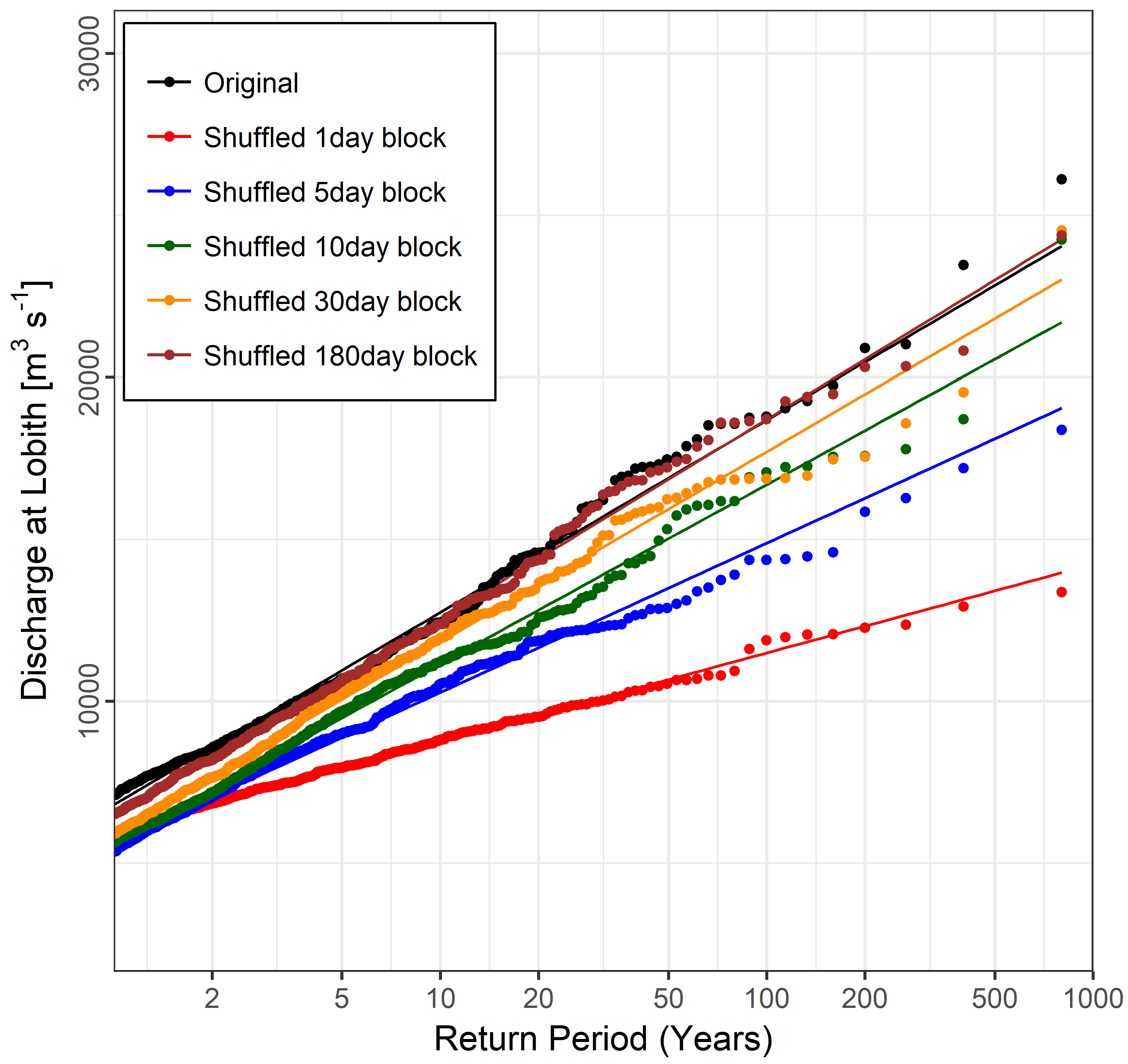
| Shuffling | Slope | Lower Bound | Upper Bound |
|---|---|---|---|
| Original | 1 | 0.978 | 1.022 |
| Shuffled 1 day block | 0.462 | 0.457 | 0.467 |
| Shuffled 5 days block | 0.777 | 0.761 | 0.793 |
| Shuffled 10 days block | 0.933 | 0.916 | 0.949 |
| Shuffled 30 days block | 0.99 | 0.972 | 1.008 |
| Shuffled 180 days block | 1.035 | 0.995 | 1.049 |
© 2019 by the authors. Licensee MDPI, Basel, Switzerland. This article is an open access article distributed under the terms and conditions of the Creative Commons Attribution (CC BY) license (http://creativecommons.org/licenses/by/4.0/).
Share and Cite
Khanal, S.; Lutz, A.F.; Immerzeel, W.W.; Vries, H.d.; Wanders, N.; Hurk, B.v.d. The Impact of Meteorological and Hydrological Memory on Compound Peak Flows in the Rhine River Basin. Atmosphere 2019, 10, 171. https://doi.org/10.3390/atmos10040171
Khanal S, Lutz AF, Immerzeel WW, Vries Hd, Wanders N, Hurk Bvd. The Impact of Meteorological and Hydrological Memory on Compound Peak Flows in the Rhine River Basin. Atmosphere. 2019; 10(4):171. https://doi.org/10.3390/atmos10040171
Chicago/Turabian StyleKhanal, Sonu, Arthur F. Lutz, Walter W. Immerzeel, Hylke de Vries, Niko Wanders, and Bart van den Hurk. 2019. "The Impact of Meteorological and Hydrological Memory on Compound Peak Flows in the Rhine River Basin" Atmosphere 10, no. 4: 171. https://doi.org/10.3390/atmos10040171
APA StyleKhanal, S., Lutz, A. F., Immerzeel, W. W., Vries, H. d., Wanders, N., & Hurk, B. v. d. (2019). The Impact of Meteorological and Hydrological Memory on Compound Peak Flows in the Rhine River Basin. Atmosphere, 10(4), 171. https://doi.org/10.3390/atmos10040171