Article

The Internal Multidecadal Variability of SST in the Pacific and Its Impact on Air Temperature and Rainfall over Land in the Northern Hemisphere

Key Laboratory of Meteorological Disaster, Ministry of Education (KLME)/Joint International Research Laboratory of Climate and Environment Change (ILCEC)/Collaborative Innovation Center on Forecast and Evaluation of Meteorological Disasters (CIC-FEMD), Nanjing University of Information Science and Technology, Nanjing 210044, China
*
Author to whom correspondence should be addressed.
Atmosphere 2019, 10(3), 153; https://doi.org/10.3390/atmos10030153
Submission received: 8 February 2019 / Revised: 11 March 2019 / Accepted: 16 March 2019 / Published: 21 March 2019
(This article belongs to the Section Meteorology)

Abstract

:
Based on the centennial-scale observations and re-analyses, this paper employs the ensemble empirical mode decomposition to separate the internal multidecadal variability (IMV) from the externally-forced variability of sea surface temperature (SST), and then defines new indices that represent the IMV of SST in the North Pacific (NPIMV) and South Pacific (SPIMV), respectively. The spatial structure of NPIMV/SPIMV shows remarkably positive SST anomaly only in the index-defined region; meanwhile, the temporal evolutions of NPIMV and SPIMV are uncorrelated, indicating their independence of each other. Both NPIMV and SPIMV play a critical role in the near-surface air temperature and rainfall over land in the Northern hemisphere, especially in the season when their intensity is the strongest. It is through teleconnection wave trains that NPIMV and SPIMV exert influences on remote regions. Results from another two rainfall datasets are found to be consistent in the majority of the Northern hemisphere in response to NPIMV/SPIMV, yet disagreement exists in certain regions due to large uncertainties of rainfall datasets.

1. Introduction

The multidecadal variability (MV) of the sea surface temperature (SST) in the Pacific and its climate impact have been of great interest in climate research in recent decades. Previous studies have defined various indices to represent the MV in the Pacific, of which the Pacific decadal oscillation (PDO) and the interdecadal Pacific oscillation (IPO) are the most widely used. PDO is defined as the leading empirical orthogonal function (EOF) of SST poleward of 20° N in the North Pacific after removing the global mean SST, with the positive phase of PDO corresponding to negative SST anomaly (SSTA) in the mid-latitude North Pacific and positive SSTA along the Western coast of North America [1,2]. IPO is defined as the second EOF mode of SST in global oceans and has a tri-pole distribution in the Pacific. The positive phase of IPO corresponds to negative SSTA in the mid-latitude North and South Pacific and positive SSTA in the central and Eastern tropical Pacific [3,4]. Some studies viewed PDO as a component of IPO in the North Pacific and considered it as the driving mechanism for the variation of IPO [5]. Based on the tri-pole pattern of IPO, Henley et al. defined a tri-pole Pacific index (TPI) as the residual of the area-averaged SST over the central and Eastern equatorial Pacific after removing the area-averaged SSTs over the Northwest and Southwest Pacific [6]. They showed that TPI was quite similar to IPO but was much easier to calculate. Shakun et al. imitated the definition of PDO to define a PDO-like index in the South Pacific as the leading EOF mode of SST in the South Pacific after the removal of the global mean [7]. They pointed out that these two PDO modes in the North and South Pacific have similar spatial patterns and are highly correlated in time.
Three types of mechanisms of the MV of SST in the Pacific (PMV) have been proposed: The stochastic forcing of the atmosphere [8,9], forcing from the tropical Pacific [10,11], and the oceanic dynamical processes, as well as air-sea coupling in mid-latitudes [12,13,14].
The PMV plays a critical role in global climate variations. For instance, different phases of IPO could speed up or slow down global warming (GW). The positive IPO could be superimposed onto GW caused by greenhouse gas increase, thus accelerating GW; while the negative IPO might partly offset GW and lead to GW stagnation for a certain period of time [15]. In the PDO/IPO positive phase, the air temperature in boreal winter was warmer/colder over Northwest/Eastern North America, and rainfall was more/less intense in Southern/Northern North America [16,17,18]. Positive PDO also corresponded to less rainfall over North and South China and more rainfall over the middle and lower reaches of the Yangtze River [19]. Wu et al. found an SST dipole in the mid-and-high-latitude South Pacific and South Atlantic that produced a wave train from the high-latitude Southern hemisphere to the tropics, thus affecting the circulation and rainfall in East Asia through the intertropical convergence zone [20].
The SST variability in general, and that associated with PDO or IPO in particular, is composed of two parts: One is the externally-forced SST variability, which is the SST response to external forcing including solar radiation, aerosols from volcanic eruption, greenhouse gas changes, and so on [21,22,23]; the other is internal SST variability, which is not related to external forcing and is intrinsically generated within the climate system [8,24,25,26]. PDO and IPO are not internal variabilities by their definition. In the PDO definition, the global mean SST is removed first before EOF analysis; however, global mean SST cannot represent appropriately the externally-forced SST variability, as the SST response to external forcing is not homogenous in space [27]. Additionally, IPO is defined as the second EOF mode of the global low-frequency SST; however, EOF analysis cannot separate the internal from external variability, with the leading EOF mode consisting of both externally-forced variability and part of the internal multidecadal variability (IMV) [28]. Therefore, PDO and IPO are not optimal indices to study the IMV of SST in the Pacific (PIMV). In order to investigate the spatial and temporal features of PIMV and its impact, the externally-forced variability has to be removed before defining the index of PIMV. The rest of the paper is organized as follows: Section 2 describes datasets used in the current work and the method to estimate the IMV of SST. In Section 3, we define new indices of the IMV in the North and South Pacific and analyze their spatial and temporal features. Their impacts on the air temperature and rainfall over land in the Northern hemisphere are also investigated. Conclusions and discussion are given in Section 4.

2. Data and Methodology

2.1. Data

The monthly Hadley Centre Sea Ice and Sea Surface Temperature dataset (HadISST) from 1870–2016 is used in the study, with a spatial resolution of 1° × 1° latitude by longitude [29]. The monthly atmospheric fields, including 2-meter air temperature, rainfall, geopotential height, and winds, are primarily obtained from European Centre for Medium-range Weather Forecasts (ECMWF) 20th century Re-Analysis (ERA-20C) from 1900 to 2010 [30], which is an atmospheric reanalysis using a coupled model by assimilating observations of surface pressure and winds. The spatial resolution is 1° × 1° latitude by longitude.
Another two sets of centennial-scale rainfall are used as well for comparison. One is the Global Rainfall Climatology Centre (GPCC) monthly rainfall Full Data Product (V7) from 1901 to 2013, based on quality-controlled data from global stations, with a spatial resolution of 1° × 1° latitude by longitude [31]. The other is the Time Series (TS) version 3.21 from the Climatic Research Unit (CRU) at the University of East Anglia, based on analysis of global weather stations records. It is for the periods 1901–2012, with a spatial resolution of 1° × 1° latitude by longitude [32]. We use an identical data length from 1901 to 2010 for all of the above datasets. The annual means and seasonal means are calculated and then climatology is removed.

2.2. Estimation of the IMV of SST

As stated in Introduction, the SST variability could be regarded to consist of two components, the externally-forced variability, and the internal variability. Several methods have been proposed previously to separate them, such as linear detrending, subtraction of the global mean, linear inverse model, EOF, ensemble empirical mode decomposition (EEMD), the multi-members ensemble mean, the multi-models ensemble mean, and so on [24,27,33,34,35,36,37]. The internal SST variability derived from each method is not identical with regard to spatial structure and spectrum. Some methods could introduce large biases to the estimated internal variability [27,28,37].
In this study, the EEMD method is applied to estimate the IMV of SST. EEMD is an improved method over the empirical mode decomposition (EMD), which is featured by temporal locality in that the characteristics do not change with adding data. EEMD could solve the problem of instability of EMD by adding different white noise series repeatedly to the original data and decomposing them into empirically-determined intrinsic mode functions (IMFs) and then averaging the ensemble to cancel out the added white noise and to keep the mean IMFs. EEMD could also solve the problem of not-instantaneous amplitude and frequency caused by Hilbert transform in EMD through using the direct quadrature algorithm. In the EMD, the original time series x(t) is decomposed as:
x ( t ) = j = 1 j = n c j + r n ,
where cj is the jth IMF, rn is residual, and n is the number of IMFs. In the EEMD, different white noise series are introduced to the original data x(t) to make an ensemble of new data:
x i ( t ) = x ( t ) + w i ( t ) ,
where xi(t) is the ith new data, wi(t) is the ith realization of noise. The jth IMF is given as:
c j ( t ) = lim N 1 N k = 1 k = N { c j ( t ) + α r k ( t ) } ,
where
c j ( t ) + α r k ( t )
is the kth trial of the jth IMF in the new data, N is the number of trials, and α is the magnitude of the noise. EEMD is able to separate time scales without a priori subjective criterion [35,36].
As the data length is a hundred and ten years in the present study, they are decomposed by EEMD at each grid point into six IMFs from high frequency to low frequency, the first two IMFs being the interannual component, from the third to the fifth IMFs being the multidecadal component, and the last IMF being the nonlinear trend. The nonlinear trend derived from EEMD is regarded as the externally-forced component in the present study. The internal variability of SST is thus obtained after removing the sixth IMF, and then the IMV of SST is estimated by the 11-year low-pass FIR filter.
The auto-correlation of the IMV is much larger than that of the monthly/seasonal/annual mean SST, and thus the effective degrees of freedom (EDOF) are greatly reduced for IMV. The t-test is used to determine the statistical significance of the regression coefficients, with EDOF computed after Bretherton et al. [38].

3. Results

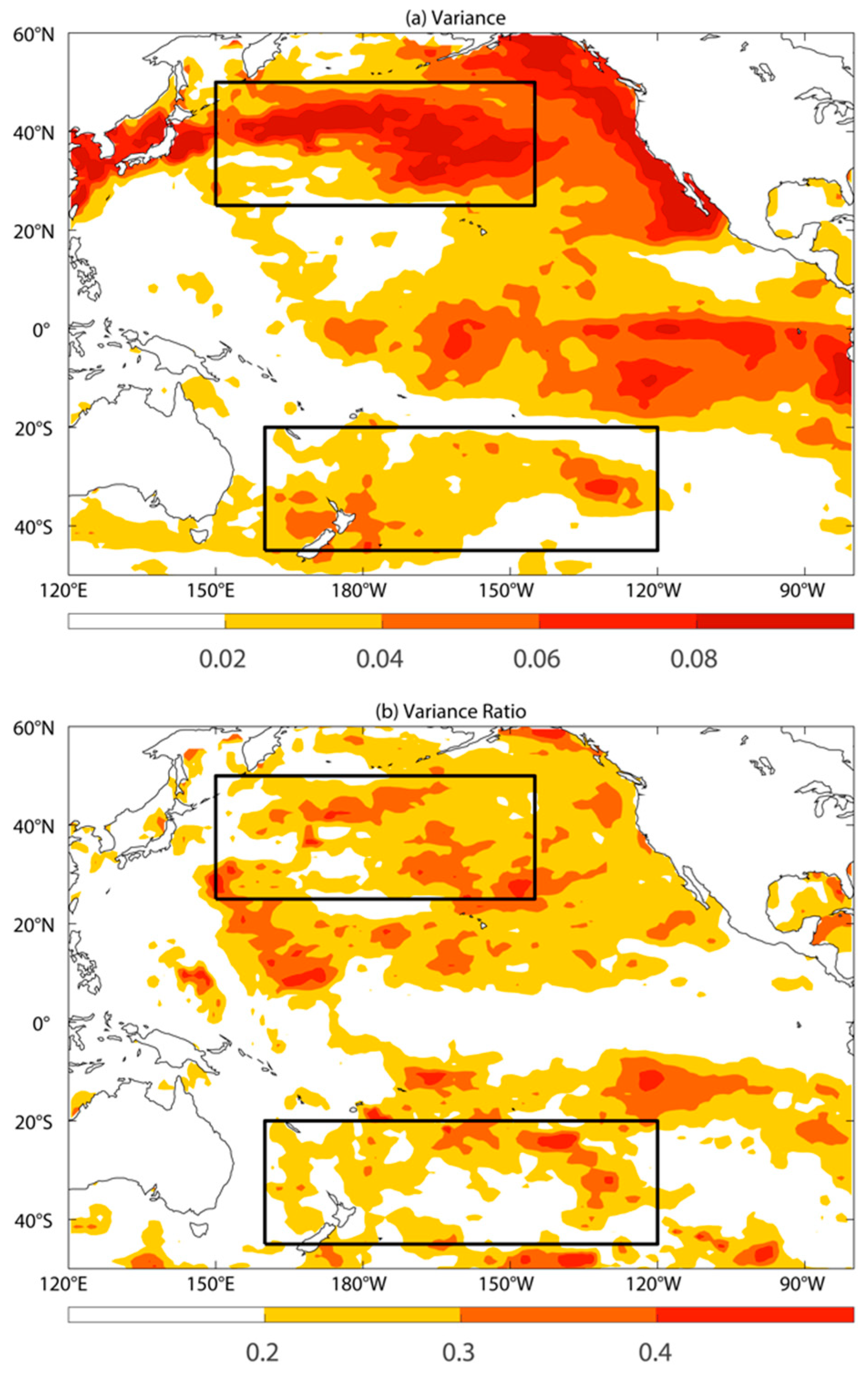
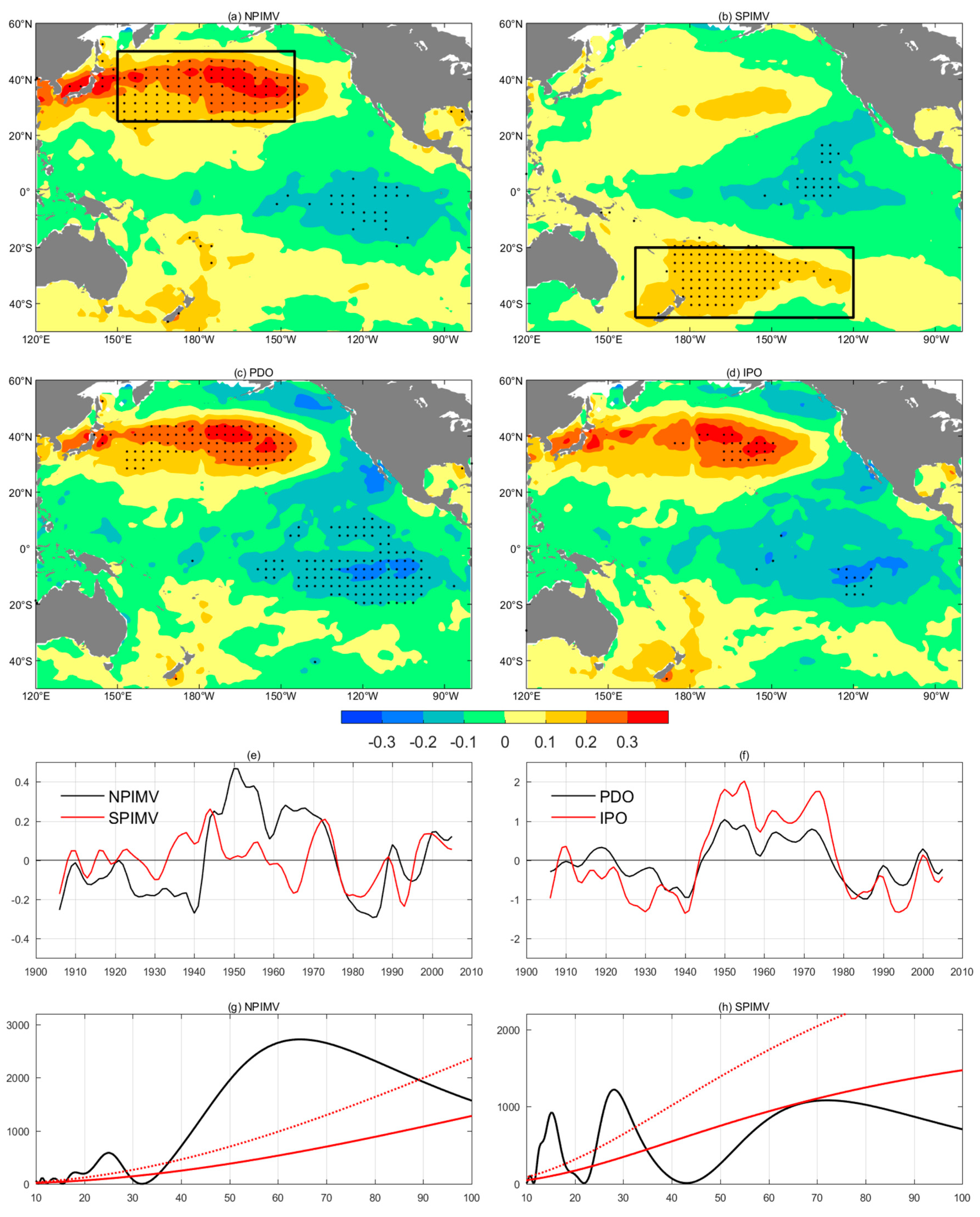
3.1. Spatial and Temporal Features of IMV in the Pacific

In order to define the IMV index in the Pacific, we first calculate the IMV variance of SST in the Pacific (Figure 1a). It can be seen that large IMV variances are located in the mid-latitude North Pacific, adjacent waters along the western coast of North America, equatorial eastern Pacific and mid-latitude South Pacific. Figure 1b shows that the variance contribution of IMV to the total SST variability (including the forced variability, the internal interannual variability, and the IMV) reaches more than 30% in the extratropical North and South Pacific, but is only 10% and even less at the equatorial Pacific. Based on the regions of both large IMV variance and large variance contribution of IMV to total variability, two indices are defined in this study: IMV in the North Pacific (NPIMV), defined as the area-averaged IMV of SSTA over (150° E–145° W, 25° N– 50° N), and IMV in the South Pacific (SPIMV), defined as the area-averaged IMV of SSTA over (160° E–120° W, 20° S–45° S) (rectangular boxes in Figure 1). It is noted that the area at (20° S–10° S) to the east of 180 ° W meets both criteria, but it is located within the tropics. In the current study, we focus on investigating the IMV in extratropical oceans in the Pacific; therefore, this area is not included in defining the indices.
Figure 2 shows the spatial distribution of the NPIMV and SPIMV modes. For NPIMV, the SSTA is significantly positive in the index-defined region in the North Pacific but is insignificant in the South Pacific. For SPIMV, the SSTA is significantly positive in the index-defined region in the South Pacific but is insignificant in the North Pacific. In terms of the spatial patterns, NPIMV and SPIMV are independent of each other. There is weak negative SSTA in the tropical Pacific for both modes, suggesting a possible extratropical-tropical connection in the Pacific.
Both indices display obvious multidecadal variations, with a long period of 60–70 years and a short period of 20–30 years. The long period is primary for NPIMV, while the short period is primary and significant for SPIMV. Since two indices are not significantly correlated simultaneously or at lags, with maximum correlation coefficient being 0.3, they are considered to be independent of each other. Therefore, we can investigate the impact of NPIMV and SPIMV separately in the following sections.
As PDO and IPO indices are commonly used to represent the multidecadal variability in the North Pacific and the entire Pacific, it is necessary to compare them with the new indices defined in the study. The spatial patterns of PDO/IPO and NPIMV are similar in the mid-latitude North Pacific, but the negative anomalies over the tropical Pacific are stronger for PDO/IPO than NPIMV, indicative of a stronger extratropical-tropical connection for PDO/IPO (Figure 2). This is expected due to the inclusion of the tropical ocean in defining the IPO index. The simultaneous correlation between NPIMV and PDO/IPO is 0.86, exceeding the 95% significance level. In terms of the spatial and temporal characteristics, the NPIMV index is able to represent the IMV in the extratropical North Pacific, with weaker interaction with the tropical ocean compared to the PDO/IPO index. The spatial pattern of PDO/IPO is different from SPIMV, and their temporal correlation is rather small and insignificant (CORR = 0.23). Thus, PDO/IPO cannot reflect the IMV in the extratropical South Pacific. It is of importance to define the SPIMV index to investigate its characteristics and climate impact.

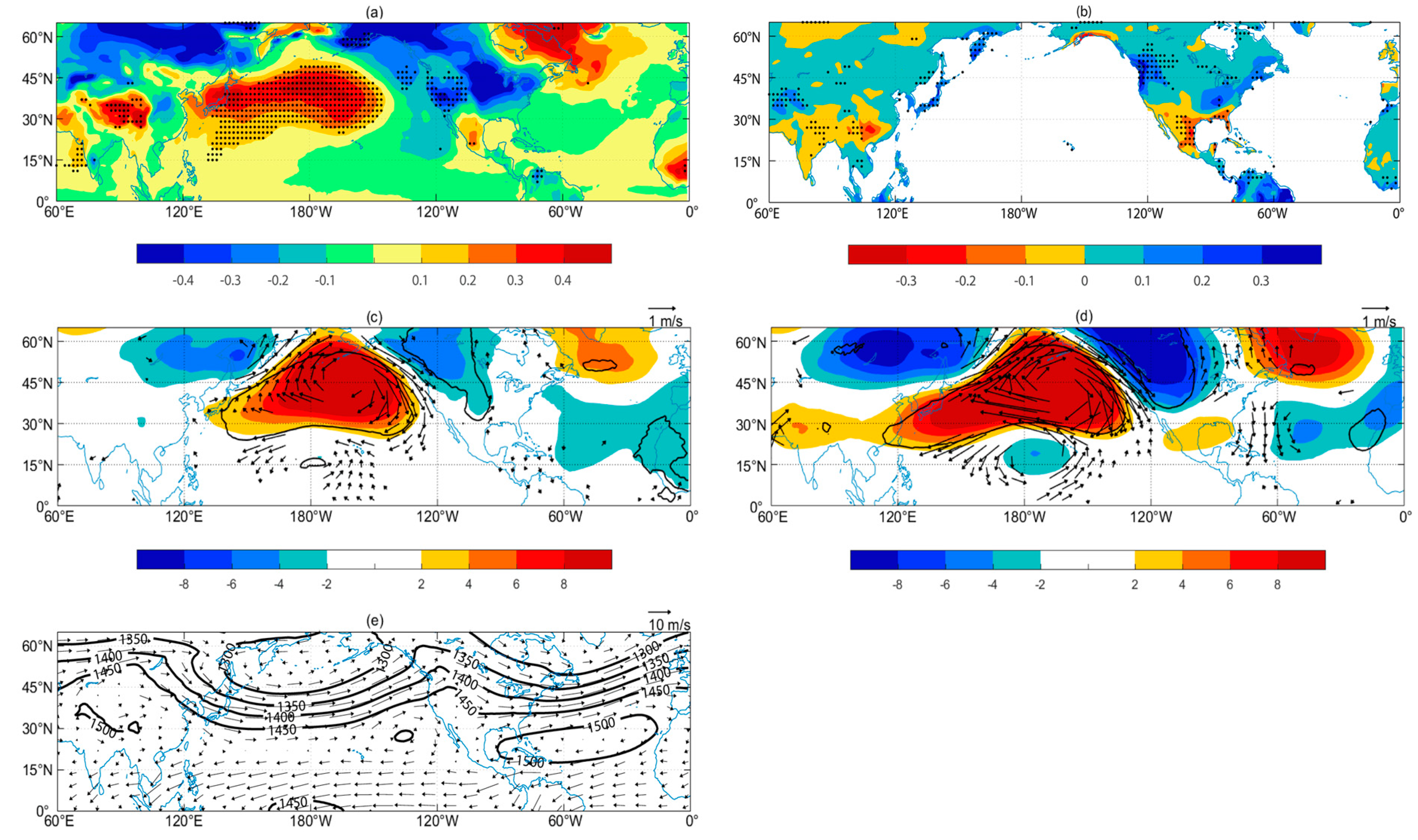
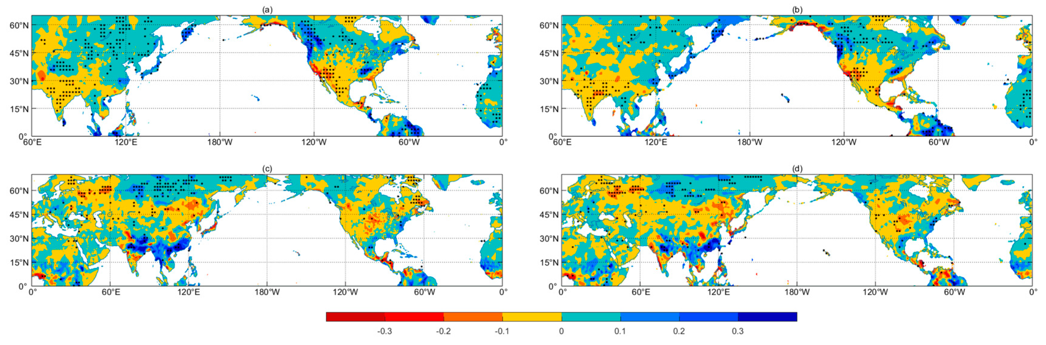
3.2. The Impact of NPIMV

The stochastic forcing of the atmosphere is one of the suggested mechanisms to drive the MV of SST in North Pacific [9]. This paper does not discuss mechanisms but focuses on the impact of NPIMV/SPIMV on the atmosphere instead. Although NPIMV plays a role in the air temperature and rainfall in all seasons, it is strongest in boreal winter (DJF). Therefore, the impact of NPIMV on air temperature and rainfall over land in DJF in the Northern hemisphere (NH) is analyzed in this section.
When NPIMV is in a positive phase (Figure 2a), the near-surface air temperature is colder than climatology over Northern North America and a majority of central and Eastern Siberia, while it is warmer than climatology over the Tibetan Plateau (Figure 3a). The rainfall is significantly more than average over Northwest and Northeast North America, while it is significantly less than average over Mexico and regions from Northern India to Southwest China (Figure 3b).
It is noted that the rainfall response to NPIMV resembles the response to La Niña over Southwestern North America [39], suggesting that the rainfall variability in this area may be attributable to both NPIMV and the SSTA over the tropical Pacific. However, the rainfall response to NPIMV is stronger than the response to La Niña over Northwestern North America, indicative of a larger impact of NPIMV on rainfall at mid-and-high latitudes.
To understand how NPIMV influences the above regions, the responses of the geopotential height and winds at 850 hPa and 500 hPa are diagnosed (Figure 3c,d). In the positive phase of NPIMV, the geopotential height anomaly is positive over the extratropical North Pacific and Mexico, and negative over Northwest North America, which is analogous to the Pacific-North America teleconnection pattern [40]. The anomalous high pressure and the associated anticyclonic wind over the mid-and-high-latitude North Pacific weaken the climatological Aleutian Low, while the anomalous low pressure and the associated cyclonic wind over Northwest North America weaken the climatological North American High (Figure 3c,e), which are consistent with previous studies on the impact of PDO [11,16,41,42]. The response of the atmospheric circulation to NPIMV can be explained by the relationship between temperature, pressure, and wind as follows: When the SSTA is positive in the extratropical North Pacific, the atmosphere above gets warmed through sensible heating (and also latent heating), leading to an increase of the depth of air column and positive height anomaly. Meanwhile, the heated atmosphere over the extratropical North Pacific weakens the baroclinicity of the atmosphere by decreasing the meridional gradient of temperature between the tropics and mid-and-high latitudes, and thus the zonal Westerly is weakened along 30°–40° N, resulting in Easterly anomaly and anticyclonic circulation (Figure 3c,d).
Due to the configuration of positive height anomaly over the mid-latitude North Pacific and negative height anomaly over Northwest North America associated with NPIMV, the air temperature over most of Northern North America is reduced by the cold advection of the anomalous Northwesterly between the anomalous high and low. Due to negative height anomaly and anomalous cyclonic circulation over Russia, the air temperature over central and Eastern Siberia is reduced by the cold advection from the Arctic (Figure 3a,c,d).
The Northwesterly anomaly over North America, which is cold and dry from a high-latitude continent, converges with the climatological warm and moist Southwesterly from low-latitude oceans, leading to enhanced rainfall over Northwest North America. The Southerly anomaly between an anomalous low over the Northwest North America and an anomalous high over the North Atlantic joins with the climatological Northwesterly, resulting in increased rainfall over Northeast North America. In climatology, Mexico lies between two highs without visible winds. A positive NPIMV produces a weak positive height anomaly over Mexico, which is unfavorable to rainfall, leading to less rainfall than average over Mexico. Moreover, the NPIMV-related positive height anomaly over the North Pacific extends Southwestward to Northern India, causing less rainfall over the regions from Northern India to Southwest China (Figure 3b–e).
Since rainfall from ERA-20C reanalysis is produced with a coupled model by assimilating observations, bias does exist. Therefore, another two sets of centennial-scale rainfall datasets are employed for comparison. Regressions of rainfall in boreal winter from CRU (Figure 4a) and GPCC (Figure 4b) onto the NPIMV index show that there is no obvious distinction of rainfall over the majority of the NH between CRU and GPCC, except over the Western Tibetan Plateau, which might be caused by sparse observation stations in this area. In the positive phase of NPIMV, rainfall increases significantly over the Northwest and Northeast North America and decreases significantly over Mexico and regions from Northern India to Southwest China, which agrees with ERA-20C. However, rainfall from CRU and GPCC are enhanced significantly over the lower reaches of the Yangtze River and regions close to Lake Baikal and reduced significantly over the area to the West of Hudson Bay in Canada, which is inconsistent with ERA-20C.

3.3. The Impact of SPIMV

The amplitude of the SPIMV index varies slightly over the four seasons. This section focuses on the impact of SPIMV on air temperature and rainfall over land in the NH in austral winter (JJA). When SPIMV is in a positive phase (Figure 2b), the air temperature is significantly warmer than usual over Northern Europe and Northeast North America, while it is remarkably colder than usual over West Siberia (Figure 5a). The rainfall increases notably over central Russia, while it is reduced over Western and Southeastern Russia (Figure 5b). It is through teleconnection wave trains that SPIMV influences the air temperature and rainfall in the NH. In the positive phase of SPIMV, a positive height anomaly could be excited locally by the positive SSTA in the mid-latitude South Pacific (Figure 5c). The local stream function anomaly at 500 hPa is negative, corresponding to anticlockwise wind circulation (Figure 5d). There is an anomalous wave train propagating Northeastward from the mid-latitude South Pacific to the mid-latitude Northwest Atlantic, with signs alternating from negative to positive to negative to positive (Figure 5d). The clockwise anomalous surface wind stress over mid-latitude Northwest Atlantic, consistent with that in the lower level, produces an Ekman transport convergence. Therefore, the sea surface height increases, the heat content increases, and SST increases. The increased SST could excite a wave train (or strengthen an existing wave train) propagating Eastward through Northern Europe and West Siberia to Eastern Russia (Figure 5d), which is similar with the Eurasian teleconnection pattern [40].
The SPIMV-related near-surface air temperature anomalies over the Eurasian continent are in good correspondence with the height anomalies, that is, positive height anomaly corresponding with anomalous warm temperature and negative height anomaly corresponding with anomalous cold temperature. Northern North America is climatologically located to the Southwest of a low-pressure area, with Northwesterly prevailing. An anomalous high is generated by SPIMV in this region, moving the climatological low Northward, and thus, the air temperature gets warmer than average (Figure 5a,c).
In Western and Southeastern Russia, positive height anomalies excited by SPIMV (Figure 5c), along with convergence at the upper level (Figure 5e), divergence at the lower level, and descending flow (Figure 5f), result in less rainfall (Figure 5b). In central Russia, a SPIMV-related negative height anomaly, along with divergence at the upper level, convergence at lower level, and ascending flow, leads to more rainfall.
As in Section 3.2, rainfall from CRU and GPCC are used for comparison as well (Figure 4c,d). In the positive phase of SPIMV, there is a notable reduction of rainfall over Western Russia and an increase of rainfall over central Russia and Northern India, consistent with ERA-20C. However, rainfall from CRU and GPCC increase remarkably over Southern China and Northern India and decrease significantly over central and Northeast North America, which disagrees with ERA-20C.

4. Conclusions and Discussion

4.1. Conclusions

The internal multidecadal variability (IMV) refers to the multidecadal variability internally generated in the climate system, which is unrelated to the external forcing. As EOF analysis cannot separate the internal from external variability, the conventional definition of PDO/IPO as the first/second EOF of low-frequency SST in the North Pacific/global ocean makes it inappropriate to represent the Pacific IMV. Therefore, this study employs EEMD to separate the IMV of SST in the observation. Based on the regions of both large IMV variance and the large contribution of IMV variance to total variance, two indices of NPIMV and SPIMV are defined to indicate the IMV of SST in the North and South Pacific, respectively. Both have a 70-year period and a 20–30-year period. For NPIMV/SPIMV, the SSTA is remarkably positive in the index-defined region in the mid-latitude North Pacific/South Pacific, while the SSTA is very weak and insignificant in the mid-latitude South Pacific/North Pacific. NPIMV is not significantly correlated with SPIMV, indicating that they are two independent IMVs.
NPIMV and SPIMV cause local height and wind anomalies and then influence the air temperature and rainfall in other regions in the NH by teleconnection wave trains. Positive NPIMV is related to colder air temperature in boreal winter over the Northern North America and the majority of the central and eastern Siberia and warmer air temperature over Tibetan Plateau. Positive NPIMV is also related to more rainfall over Northwest and Northeast North America and less rainfall over Mexico and regions from Northern India to southwest China. Positive SPIMV is associated with colder air temperature in austral winter over West Siberia and warmer air temperature over Northern Europe and Northeast North America. When SPIMV is in a positive phase, the rainfall is enhanced over central Russia and is reduced over Western and Southeastern Russia.
The responses of another two rainfall datasets from CRU and GPCC to NPIMV and SPIMV are consistent with each other in the majority of the NH, but they do not agree in certain regions with the response of rainfall from ERA-20C.

4.2. Discussion

The above conclusions are drawn based on observations and re-analysis. It is of importance to further investigate whether the observed spatial structure and the impact of NPIMV and SPIMV could be simulated by coupled models. Here we use the output from the pre-industrial control simulation in a coupled model (EC-ERATH) from the Coupled Model Intercomparison Project Phase 5 (CMIP5), which only has internal variability [43].
Figure 6 displays the spatial pattern of NPIMV and SPIMV and their impact on the air temperature and rainfall in the model. The positive SSTA over the mid-latitude North Pacific for NPIMV and the positive SSTA over the mid-latitude South Pacific for SPIMV are captured in the model, with smaller areas than the observation (Figure 6a,b). The air temperature response to NPIMV in the model is different from reanalysis over the majority of the land (Figure 3a and Figure 6c), while the patterns of rainfall response to NPIMV in the model and in reanalysis are similar over North America and dissimilar over the Eurasian continent (Figure 3b and Figure 6e). Neither the air temperature response nor the rainfall response to SPIMV in the model agrees with the reanalysis in most regions (Figure 5a,b and Figure 6d,f). Therefore, the EC-ERATH model is able to reproduce the observed spatial patterns of NPIMV and SPIMV to a certain extent, but it cannot simulate their climate impact.
This study analyzes diagnostically how NPIMV and SPIMV affect the near-surface air temperature and rainfall over land in the NH using circulation fields, which should also be verified by sensitivity experiments of numerical models. Moreover, we use three types of rainfall datasets from different research centers, yet the results obtained in this study should be treated with caution due to the large uncertainties of rainfall. Lastly, the performance of other CMIP5 models in simulating the observed characteristics of NPIMV and SPIMV needs to be examined as well.

Author Contributions

Conceptualization, methodology, visualization, writing—original draft, H.C.; data curation, formal analysis, D.H.; validation, writing—review & editing, Z.Z.

Funding

This research was funded by the National Key R&D Program of China (2016YFA0600402), and the National Natural Science Foundation of China (41405052).

Acknowledgments

This paper is ESMC Contribution No. 255.

Conflicts of Interest

The authors declare no conflict of interest.

References

  1. Mantua, N.J.; Hare, S.R.; Zhang, Y.; Wallace, J.M.; Francis, R.C. A Pacific interdecadal climate oscillation with impacts on salmon production. Bull. Am. Meteorol. Soc. 1997, 78, 1069–1079. [Google Scholar] [CrossRef]
  2. Zhang, Y.; Wallace, J.M.; Battisti, D.S. ENSO-like interdecadal variability: 1900–1993. J. Clim. 1997, 10, 1004–1020. [Google Scholar] [CrossRef]
  3. Power, S.; Casey, T.; Folland, C.; Colman, A.; Mehta, V. Inter-decadal modulation of the impact of ENSO on Australia. Clim. Dyn. 1999, 15, 319–324. [Google Scholar] [CrossRef]
  4. Parker, D.; Folland, C.; Scaife, A.; Jeff Knight, J.; Colman, A.; Baines, P.; Dong, B. Decadal to multidecadal variability and the climate change background. J. Geophys. Res. 2007, 112, D18115. [Google Scholar] [CrossRef]
  5. Folland, C.K.; Renwick, J.A.; Salinger, M.J.; Mullan, A.B. Relative influences of the interdecadal Pacific oscillation and ENSO on the south pacific convergence zone. Geophys. Res. Lett. 2002, 29, 21-1–21-4. [Google Scholar] [CrossRef]
  6. Henley, B.J.; Gergis, J.; Karoly, D.J.; Power, S.; Kennedy, J.; Folland, C.K. A tripole index for the interdecadal Pacific oscillation. Clim. Dyn. 2015, 45, 3077–3090. [Google Scholar] [CrossRef]
  7. Shakun, J.D.; Shaman, J. Tropical origins of North and South Pacific decadal variability. Geophys. Res. Lett. 2009, 36, L19711. [Google Scholar] [CrossRef]
  8. Hasselmann, K. Stochastic climate models. Part I. Theory. Tellus 1976, 28, 473–485. [Google Scholar] [CrossRef]
  9. Frankignoul, C.; Reynolds, R.W. Testing a dynamical model for mid-latitude sea surface temperature anomalies. J. Phys. Oceanogr. 1983, 13, 1131–1145. [Google Scholar] [CrossRef]
  10. Trenberth, K.E.; Branstator, G.W.; Karoly, D.; Arun Kumar, A.; Lau, N.-C.; Ropelewski, C. Process during TOGA in understanding and modeling global teleconnections associated with tropical sea surface temperatures. J. Geophy. Res. 1998, 103, 14291–14324. [Google Scholar] [CrossRef]
  11. Newman, M.; Compo, G.P.; Alexander, M. ENSO-forced variability of the Pacific decadal oscillation. J. Clim. 2003, 16, 3853–3857. [Google Scholar] [CrossRef]
  12. Latif, M.; Barnett, T.P. Causes of decadal climate variability over the North Pacific and North America. Science 1994, 266, 634–637. [Google Scholar] [CrossRef]
  13. Schneider, N.; Cornuelle, B.D. The forcing of the Pacific decadal oscillation. J. Clim. 2005, 18, 4335–4373. [Google Scholar] [CrossRef]
  14. Miyasaka, T.; Nakamura, H.; Taguchi, B.; Nonaka, M. Multidecadal modulations of the low-frequency climate variability in the wintertime North Pacific since 1950. Geophys. Res. Lett. 2014, 41, 2948–2955. [Google Scholar] [CrossRef]
  15. Meehl, G.A.; Hu, A.; Arblaster, J.M.; Fasullo, J.; Trenberth, K.E. Externally forced and internally generated decadal climate variability associated with the interdecadal Pacific oscillation. J. Clim. 2013, 26, 7298–7310. [Google Scholar] [CrossRef]
  16. Li, C.; Xian, P. Interdecadal variation of SST in the North Pacific and the anomalies of atmospheric circulation and climate. Clim. Environ. Res. 2003, 8, 909–915. [Google Scholar]
  17. Dai, A. The influence of the inter-decadal Pacific oscillation on US rainfall during 1923–2010. Clim. Dyn. 2013, 41, 633–646. [Google Scholar] [CrossRef]
  18. Xu, Y.; Hu, A. How would the twenty-first-century warming influence Pacific decadal variability and its connection to North American rainfall: Assessment based on a revised procedure for the IPO/PDO. J. Clim. 2018, 31, 1547–1563. [Google Scholar] [CrossRef]
  19. Qian, C.; Zhou, T. Multidecadal variability of North China aridity and its relationship to PDO during 1900–2010. J. Clim. 2013, 27, 1210–1222. [Google Scholar] [CrossRef]
  20. Wu, Z.; Dou, J.; Lin, H. Potential influence of the November-December southern hemisphere annular mode on the East Asian winter rainfall: A new mechanism. Clim. Dyn. 2015, 44, 1215–1226. [Google Scholar] [CrossRef]
  21. Houghton, J.T.; Jenkins, G.J.; Ephraums, J.J. Climate Change: The IPCC Scientific Assessment; Cambridge University Press: Cambridge, UK, 1990. [Google Scholar]
  22. Robock, A.; Mao, J. Winter warming from large volcanic eruptions. Geophys. Res. Lett. 1992, 12, 2405–2408. [Google Scholar] [CrossRef]
  23. Lean, J.; Beer, J.; Bradley, R. Reconstruction of solar irradiance since 1600: Implications for climate change. Geophys. Res. Lett. 1995, 22, 3195–3198. [Google Scholar] [CrossRef]
  24. Colfescu, I.; Schneider, E.K.; Chen, H. Consistency of 20th century sea level pressure trends as simulated by a coupled and uncoupled GCM. Geophys. Res. Lett. 2013, 40, 1–5. [Google Scholar] [CrossRef]
  25. Chen, H.; Schneider, E.K.; Wu, Z. Mechanisms of internally generated decadal-to-multidecadal variability of SST in the Atlantic ocean in a coupled GCM. Clim. Dyn. 2016, 46, 1517–1546. [Google Scholar] [CrossRef]
  26. Mckinnon, K.A.; Deser, C. Internal variability and regional climate trends in an observational large ensemble. J. Clim. 2018. [Google Scholar] [CrossRef]
  27. Ting, M.F.; Kushnir, Y.; Seager, R.; Li, C. Forced and internal twentieth-century SST trends in the North Atlantic. J. Clim. 2009, 22, 1469–1481. [Google Scholar] [CrossRef]
  28. Frankignoul, C.; Gastineau, G.; Kwon, Y.O. Estimation of the SST response to anthropogenic and external forcing, and its impact on the Atlantic multidecadal oscillation and the Pacific decadal oscillation. J. Clim. 2017, 30, 9871–9895. [Google Scholar] [CrossRef]
  29. Rayner, N.A.; Parker, D.E.; Horton, E.B.; Folland, C.K.; Alexander, L.V.; Rowell, D.P.; Kent, E.C.; Kaplan, A. Global analyses of sea surface temperature, sea ice, and night marine air temperature since the late nineteenth century. J. Geophys. Res. 2003, 108, 1063–1082. [Google Scholar] [CrossRef]
  30. Poli, P.; Hersbach, H.; Tan, D.G.H.; Dee, D.P.; Thépaut, J.-N.; Simmons, A.; Peubey, C.; Laloyaux, P.; Komori, T.; Berrisford, P.; et al. The Data Assimilation System and Initial Performance Evaluation of the ECMWF Pilot Reanalysis of the 20th-Century Assimilating Surface Observations Only (ERA-20C); ERA Report Series; ECMWF: Berkshire, UK, 2013. [Google Scholar]
  31. Schneider, U.; Becker, A.; Finger, P.; Meyer-Christoffer, A.; Rudolf, B.; Ziese, M. GPCC Full Data Reanalysis Version 6.0 at 1.0°: Monthly Land-Surface Rainfall from Rain-Gauges Built on GTS-Based and Historic Data; Global Precipitation Climatology Centre (GPCC): Berlin, Germany, 2011. [Google Scholar] [CrossRef]
  32. Jones, P.D.; Harris, I.C. Climatic Research Unit (CRU) Time-Series Datasets of Variations in Climate with Variations in Other Phenomena; NCAS British Atmospheric Data Centre: Oxford, UK, 2008. [Google Scholar]
  33. Trenberth, K.E.; Shea, D.J. Atlantic hurricanes and natural variability in 2005. Geophys. Res. Lett. 2006, 33, L2704. [Google Scholar] [CrossRef]
  34. Schneider, E.K.; Fan, M. Weather noise forcing of surface climate variability. J. Atmos. Sci. 2007, 64, 3265–3280. [Google Scholar] [CrossRef]
  35. Wu, Z.; Huang, N.E. Ensemble empirical mode decomposition: A noise-assisted data analysis method. Adv. Adapt. Data Anal. 2009, 1, 1–41. [Google Scholar] [CrossRef]
  36. Wu, Z.; Huang, N.E.; Wallace, J.M.; Smoloak, B.V.; Chen, X. On the time-varying trend in global–mean surface temperature. Clim. Dyn. 2011, 37, 759–773. [Google Scholar] [CrossRef]
  37. Francombe, L.M.; England, M.H.; Mann, M.E.; Steinman, B.A. Separating internal variability from the externally forced climate response. J. Clim. 2015, 28, 8184–8202. [Google Scholar] [CrossRef]
  38. Bretherton, C.S.; Widmann, M.; Dymnikov, V.P.; Wallace, J.M.; Bladé, I. The effective number of spatial degrees of freedom of a time-varying field. J. Clim. 1999, 12, 1990–2009. [Google Scholar] [CrossRef]
  39. Feldl, N.; Roe, G.H. Climate variability and the shape of daily precipitation: A case study of ENSO and the American West. J. Clim. 2011, 24, 2483–2499. [Google Scholar] [CrossRef]
  40. Wallace, J.M.; Gutzler, D.S. Teleconnections in the geopotential height field during the northern hemisphere winter. Mon. Weather Rev. 1981, 109, 784–812. [Google Scholar] [CrossRef]
  41. Zhu, Y.; Yang, X. Relationship between Pacific decadal oscillation and climate variabilities in China. Acta Meteorol. Sin. 2003, 61, 641–654. [Google Scholar]
  42. Newman, M.; Alexander, M.A.; Ault, T.R.; Cobbd, K.M.; Desere, C.; Di Lorenzod, E.; Mantuaf, N.J.; Millerg, A.J.; Minobeh, S.; Nakamurai, H.; et al. The Pacific decadal oscillation, revisited. J. Clim. 2016, 29, 4399–4427. [Google Scholar] [CrossRef]
  43. Taylor, K.E.; Stouffer, R.J.; Meehl, G.A. An overview of CMIP5 and the experimental design. Bull. Am. Meteorol. Soc. 2012, 93, 485–498. [Google Scholar] [CrossRef]
Figure 1. (a) The internal multidecadal variance of sea surface temperature (SST) anomalies in the Pacific. Unit: (°C)2. (b) The ratio between the internal multidecadal variance and total variance of SST. The rectangular boxes in the mid-latitude North and South Pacific are regions in which the indices of the internal multidecadal variability in the North and South Pacific (NPIMV and SPIMV) are defined.
Atmosphere 10 00153 g001
Figure 2. Regressions of SST anomalies onto (a) the NPIMV index, (b) the SPIMV index, (c) the Pacific decadal oscillation (PDO) index, and (d) the interdecadal Pacific oscillation (IPO) index (unit: °C per standard deviation). Values exceeding 90% for the significance test are dotted. (e) Time series of the NPIMV (black curve) and SPIMV (red curve) indices (unit: °C). (f) Time series of the standardized PDO (black curve) and IPO (red curve) indices. The PDO and IPO indices are multiplied by (−1) in order to compare with NPIMV and SPIMV. Power spectrum of (g) the NPIMV index and (h) the SPIMV index are shown. In (g) and (h), the red solid curve is corresponding red noise spectrum and the red dotted curve shows 5% confidence upper limit of the red noise spectrum. The x-axis is period (unit: years) and the y-axis is power.
Atmosphere 10 00153 g002
Figure 3. Regressions of the boreal winter; (a) 2-meter air temperature (°C), (b) rainfall (mm/day), geopotential height (gpm) and wind (m/s) (c) at 850 hPa and (d) at 500 hPa onto the NPIMV index. (e) Climatological mean geopotential height (gpm) and wind (m/s) at 850 hPa. (a,b): Values exceeding 90% for the significance test are dotted. (c,d): Winds exceed 90% for the significance test; the black contours indicate the geopotential height exceeding 90% for the significance test.
Atmosphere 10 00153 g003
Figure 4. (a,b) Regressions of rainfall in boreal winter from (a) the Climatic Research Unit (CRU) and (b) the Global Rainfall Climatology Centre (GPCC) onto the NPIMV index. (c,d) Regressions of rainfall in austral winter from (c) CRU and (d) GPCC onto the SPIMV index. Values exceeding 90% for the significance test are dotted. Unit: mm/day.
Atmosphere 10 00153 g004
Figure 5. Regressions of the austral winter. (a) 2-meter air temperature (°C), (b) rainfall (mm/day), (c) geopotential height (gpm) and wind (m/s) at 850 hPa, (d) streamfunction (105 m2/s) at 500 hPa, (e) velocity potential (contours, unit: 105 m2/s) and divergent wind (vectors, unit: m/s) at 200 hPa, and (f) vertical velocity at 500 hPa (Pa/s) onto the SPIMV index. (a,b): Values exceeding 90% for the significance test are dotted. (c): Winds exceed 90% for the significance test; the black contours indicate the geopotential height exceeding 90% for the significance test. (f): Red shadings indicate descending motion and blue shadings indicate ascending motion.
Atmosphere 10 00153 g005
Figure 6. Regressions of SST anomaly (SSTA) onto (a) the NPIMV index and (b) the SPIMV index (unit: °C per standard deviation). Regressions of the boreal winter (c) 2-meter air temperature (°C) and (e) rainfall (mm/day) onto the NPIMV index. Regressions of the austral winter (d) 2-meter air temperature (°C) and (f) rainfall (mm/day) onto the SPIMV index. Values exceeding 90% for the significance test are dotted. Data are obtained from the CMIP5 pre-industrial control simulation in the EC-ERATH model.
Atmosphere 10 00153 g006

