Article

Isoprene, Methyl Vinyl Ketone and Methacrolein from TROICA-12 Measurements and WRF-CHEM and GEOS-CHEM Simulations in the Far East Region

A.M. Obukhov Institute of Atmospheric Physics, Russian Academy of Sciences, Pyzhevskii per. 3, 119017 Moscow, Russia
*
Author to whom correspondence should be addressed.
Atmosphere 2019, 10(3), 152; https://doi.org/10.3390/atmos10030152
Submission received: 12 March 2019 / Accepted: 16 March 2019 / Published: 21 March 2019
(This article belongs to the Section Air Quality)

Abstract

:
Spatial and temporal distributions of isoprene and its oxidation products, methyl vinyl ketone and methacrolein in the Far East region of Russia were investigated. The measurement data were obtained from a mobile laboratory, which moved along the Trans-Siberian railway and from WRF-CHEM (Weather Research and Forecasting Chemical Model) and GEOS-CHEM (Goddard Earth Observing System Chemical Model) simulations. During the simulations, the RACM-MIM and MOZART mechanisms, included in the mesoscale WRF-CHEM model, as well as the Caltech Isoprene Scheme (CIS), built in the global GEOS-CHEM model, have been used. We found that the temporal distribution of the measured isoprene is in good agreement with the simulations. The measured isoprene, methyl vinyl ketone (MVK) and methacrolein (MACR) concentrations demonstrate pronounced diurnal variations. The correlation between the measured isoprene and MVK + MACR was good (R ~ 0.60–0.86). However, the simulated correlation between MVK + MACR and isoprene is very low, with the data for the night-time and daytime values varying. The simulated MVK + MACR to isoprene ratio, in comparison with the experimental result, has pronounced diurnal variations. During twilight and the night-time, the simulated MVK + MACR to isoprene ratio is more than 10. We propose that, due to the validity of the kinetic equations only in the homogeneous system, all chemical and transport (CTM) models, based on these kinetic equations, are not able to show an adequate simulation at night in the weak mixing atmosphere, when the atmospheric structure becomes heterogeneous. At moderate latitudes, we recommend the use of the turbulent Damköhler number and the Kolmogorov Damköhler numbers, which characterize the limits of CTM applicability, as the quality flags at the air quality forecast simulations.

1. Introduction

Isoprene, which is known to be formed inside of leaf chloroplasts, is the most abundant plant-emitted hydrocarbon in the atmosphere, with global carbon emissions reaching 500 to 750 Tg per year [1].
Because in the daytime, the isoprene lifetime is determined by the oxidation by OH, with a reaction rate of kOH = 101 × 10−12 cm−3 molec.−1·s−1, the lifetime is insignificant and it is equally only 1.2–1.5 h [2]. As a result, at the advection of air masses, with a wind speed of 3–5 m·s−1, it is possible to register isoprene, which was emitted by vegetation from a distance not exceeding 30 km. Thus, isoprene measurements, carried out at a stationary observation point, are tied to local types of vegetation species that grow in close proximity to this observation point.
It is of interest to carry out an investigation on the spatial and temporal distribution of isoprene using a moving laboratory, crossing the areas covered by various types of vegetation. The range of isoprene emissions is determined not only by the diversity of vegetation and by the variability of solar radiation and temperature but is also determined by the variety of soils, the moisture presence in the soils and by a zonal microclimate in the mountain-valley area. It should be noted that isoprene emissions also depend on various repressive factors, such as vegetation damage by previous wildfires and by insects, felling, droughts, strong frosts and other unfavourable conditions.
As a result, the local characteristics of the biogenic emission rate may differ from regional and average statistical emissions rates of biogenic database emissions. Therefore, it is of interest to analyse isoprene emissions using a mobile observatory. A site in the Far East, along the Trans-Siberian railway, passing through an area corresponding to a subtropical climate, was chosen as a testing ground. This study was carried out as part of the TROICA-12 expedition. More detailed information about the TROICA expeditions and the biogenic and anthropogenic emissions along the Trans-Siberian railway can be found in References [3,4,5,6,7].
The first goal of this study is to validate the MEGAN emission inventories, built into the WRF-CHEM (Weather Research and Forecasting Chemical Model) and GEOS-CHEM (Goddard Earth Observing System Chemical Model). The first part of the study is of interest only for a limited group of atmospheric chemical models.
The simultaneous continuous measurements of isoprene as well as methyl vinyl ketone (MVK) and methacrolein (MACR) and the meteorological parameters in the unique TROICA experiments, performed by a mobile laboratory in the summer of 2008, allow the spatial and temporal variations of isoprene oxidation products to be studied.
The second goal of this study is carried out in studies of the in-field chemical mechanisms of isoprene oxidation, which undoubtedly has a great discussion potential. This is especially topical, since most of the TROICA measurements were made under “low-NO” conditions.
Isoprene biogenic emissions depend on sunlight and temperature, and, as a result, most biogenic emissions occur during the daytime [1,8]. In the atmosphere, isoprene can react with hydroxyl radicals (OH), ozone and nitrate radicals (NO3), which leads to the formation of gases, such as formaldehyde, MVK, MACR, carbon monoxide (CO) and ozone (O3) [9].
In the daytime, isoprene chemistry is determined by the interaction of isoprene with OH and O3 at night—by the interaction with NO3 and O3. As will be shown below, a significant discrepancy in night and twilight conditions, between the simulated and experimental values of the ratio of the sum of MVK and MACR to isoprene, was revealed. The experimental data were compared with the simulation results, obtained from two regional and one global transport-chemical model. Additionally, noises in chemical reactions were detected at night and under twilight conditions.
In the study, it was suggested with caution that the problem in nocturnal isoprene chemistry is associated with poor mixing in the atmospheric boundary layer and the heterogeneous and quasi-heterogeneous nature of chemical reactions at night.

2. Measurements, Datasets and Methods

2.1. NOx, Ozone and Meteorological Measurements

The TROICA experiments through the territory of Russia in a mobile laboratory have been carried out regularly since 1995 [10]. About 10 inorganic compounds (ozone, nitric oxides, carbon oxides, methane, sulphur dioxide, etc.), 21 volatile organic compounds (VOCs) as well as aerosols and meteorological parameters, such as air temperature, atmosphere pressure and humidity, solar radiation, vertical temperature profiles, wind speed and direction at train stops, were measured continuously and simultaneously by a specially constructed automated system. The system was built on a railway carriage, with air inlets on the carrier roof at a height of about 4 m above the ground. The TROICA carriage laboratory is equipped in accordance with the measurement requirements of the Global Atmospheric Watch (GAW) and located just after the electric locomotive to minimize various effects of near-surface air perturbations due to train movement. The possible impact of oncoming trains and human activities in the train is generally non-significant, as demonstrated previously in References [3,11].
In the present study, the spatial and temporal distribution of isoprene from the summer experiment, TROICA-12 (July 21–August 4, 2008), along the Trans-Siberian railway, are analysed (Figure 1).
Hot weather (>24 °C at noon) was found along the Trans-Siberian railroad during both periods of expeditions, Troica-12 East and West. Night-time surface temperature inversions and stagnant air conditions and light winds during the daytime were typical of both the east and the west segments of the experiment in the Far East region.
The stretch of the Trans-Siberian Railway from Lake Baikal to the coast of the Pacific Ocean passes through the sparsely populated territory of Russia, overgrown with broadleaf and coniferous vegetation. The spatial distribution along the railway of NO, NOx (NOx = NO + NO2), O3 and CO is shown in Figure 2. In the Figure 2 the distance was measured along the Trans-Siberian Railway from Moscow, where it was the start point of the TROICA-12 expedition (Moscow–Vladivostok–Moscow). The distance in the both directions (East and West routes) was calculated from the values of the GPS sensor, installed on the roof of the wagon-observatory.
The low values of NO, NOx as well as CO concentrations show that, in general, the expedition occurred under uncontaminated conditions. Note that 0.2 ppm for CO is the background for TE48S, which was used for CO measurements. The sharp peaks in NO and NOx concentrations correspond to local emission sources, such as railway stations and settlements. We recorded one long-distance plume from the central part of China, which crossed the Trans-Siberian Railroad in the TROICA-12 West expedition. The plume crossed the railroad at the distance label ~8300 km and is shown in Figure 2. The CO max value for this long-distance plume is equal to ~0.4 ppm.
For isoprene oxidation chemistry, the NO level is important, as it is used for the differentiation between two channels of chemical reactions: NO-dominant and HO2-dominant pathways. In some works, for example [12], the NO level to separate these two pathways was found to be sufficiently high and was equal to 5 ppb. However, in Reference [13], this NO level was defined as 0.5 ppb.
Statistical analysis of TROICA-12 data shows that, in an investigated site of the Trans-Siberian railroad, the number of measurements with NO < 5 ppb is equal to 94% and 96% of the total measurements for the East and West stage, respectively. Additionally, it was found that the number of measurements with NO < 0.5 ppb is equal to 74% and 67% for the East and West stage, respectively. Moreover, most sources with high NOx values have a local origin and the powerful NOx plumes from the central areas of China were not observed (Figure 2).
Analysis of long-transport plume, described above, was conducted using the NOAA hysplit model, showing that the backward trajectories started at 48.59° N, 133.63° E at 250 and 500 m above ground level (a.g.l.) and passed at low altitudes over the central part of China that has many industrial plants. The contaminated air mass reached the Trans-Siberian Railway at 29.07.2008 07 UTC after ~54 h of flight. Since the propagation time exceeds the NOx lifetime, the NOx plume was not detected in the concentration distribution during measurement scanning along the railroad. As is well-known, in summer, the CO gas has a lifetime equal to ~10–14 days and usually uses an indicator of long-range pollution transport. We recorded raised CO values in the short part of the Troica-12 West route, 8100–8700 km and assumed that it is a long-range pollution transport from the central part of China (Figure 2).

2.2. VOCs Measurements and PTR-MS

As is well-known, proton transfer reaction mass spectrometry (PTR-MS) provides an on-line monitoring of VOCs with a low detection threshold and a fast response time. Detailed information about PTR-MS can be found in Reference [14] and in the reviews [15,16,17].
In TROICA experiments, the Compact PTR-MS from Ionicon Analytik GmbH, Innsbruck (Austria) was used. The main advantage of the instrument is its portability, the possibility of real-time measurements, real-time quantification and low fragmentation. It is easy to operate and no sample preparation is necessary. It allows Compact PTR-MS to be very useful for continuous measurements on moving platforms [18,19].
The instrument allows the simultaneous on-line monitoring of 21 VOCs, including acetylene (m27), formaldehyde+ (m31), methanol+ (m33), acetonitrile (m42), acetaldehyde (m45), ethanol (m47), 1,3 butadiene (m55), butane (m57), acetone (m59), cyclopentadienil (m66), benzene (m79), terpenes (m81, m137), toluene (m93), phenol (m95), styrene (m105), xyluene, C8 benzenes (m107), propylbenzene (m121) and trichloroacetic acid (m163). The VOCs, which have isomers, are marked by a plus.
The fact that, due to their low proton affinities, H3O+ ions do not react with any of the major components present in clean air is an additional advantage, as it allows the analysed air to be used directly as the buffer gas. To set a correct transmission in the software, a gas standard (Ionicon Analytic GmbH, Innsbruck), containing 17 VOCs, including benzene (m79), toluene (m93) and isoprene (m69), was used. The error in calibration by the gas standard did not exceed 15%.
The instrument consists of an ion source, a drift tube reaction chamber and a quadrupole mass spectrometer (QMS). H3O+ ions were generated in the hollow cathode discharge and directed to the drift tube, where H3O+ and VOC ion-molecule reactions take place.
Thus, the method is based on the following chemical reaction:
R + H 3 O + R H + + H 2 O
where R is the atmospheric VOCs and RH+ represents the VOCs concentration, measured by QMS.
The determination of R species by the H3O+ method is possible only if the chemical compound has an affinity with the proton above than with water. The basic VOCs components, studied in this work, such as isoprene and their oxidation products, have a higher affinity with the proton above than with water and they can therefore be determined using a PTR-MS technique. However, the proton mass spectrometry method has a lack of selectivity in the case of chemical compounds having the same atomic weight and hence, isomers do not separate during our measurements. In our study, the PTR-MS method with the H3O+ injector does not allow us to separate the oxidation products of biogenic emissions, such as MVK and MACR, so we use the sum of them for an analysis. The reagent and product ions were detected by the QMS in the 1–300 amu (atomic mass unit) range, with a resolution of <1 amu. The linearity range of VOC value measurements is equal to 500 pptv–10 ppmv and the measuring time is about 10 s. The IONICON Analytik GmbH product description can be found in Reference [20].
Nevertheless, the isoprene signal should be interpreted carefully, particularly from coniferous forests, where the emissions of 2-methyl-3-buten-2-ol (232 MBO), which is also determined at m/z 69, take place [21,22,23,24]. According to Karl et al. [24] the average ratio between isoprene and 232 MBO is about 0.2 during the daytime and about 0.5 during the night-time. However, in broadleaf forests, the isoprene was often found to be the dominant species at m/z 69 within various kinds of air masses [16]. The sum of MVK and MACR was detected by the instrument at m/z 71.
PTR-MS was installed in the unified air intake system of our measurement complex [10]. The air samples were taken from the roof of the carriage through a system of Teflon tubes. The observatory wagon followed at once for the electric locomotive. The height of the observatory wagon was higher than the height of the electric locomotive, which allows air to be taken from an unperturbed, direct inflowing stream. The gap between the trains following in one direction is great, therefore, the turbulence of the previous train was not observed. The air intake system compensates the dynamic pressure caused by the train movement. A strong disturbance of the flow and dynamic pressure was observed only when the train passed tunnels, viaducts, under bridges, canyons and oncoming trains. The recorded dataset was automatically filtered from these errors by the GIS, which was automatically turned off in the tunnels and under bridges. The trains coming from the opposite direction were automatically registered by the microbarograph and investigated by the observation operators, which define the type of oncoming train (passenger, tank or coal car).
Note that, unlike GC in a certain sense, PTR-MS does not require calibration for individual chemical species, since it is a mass spectrometer. Adjustment of PTR-MS injector and quadrupole system of the signal registration was carried out by the manufacturer. The basic error of the PTR-MS is determined by the carriage vibrations during carriage movement and by the noise in the electrical system of the measurement complex. The observatory carriage was made at the rail-carload company, according to the special design project, which allows for the suppression of vibrations due to carriage suspension brackets. Noises in the electrical network were suppressed by a powerful carriage generator, special electric converters and under-carriage batteries.
A complete description of the measurement technique, data quality assessment and the dataset obtained from the measurements from the railroad mobile laboratory are presented in our previous publication [10] and some details about using PTR-MS in TROICA experiments can also be found in Reference [6,7].

2.3. Regional WRF-CHEM Model

For the simulations, in this study, we selected one of the best hydrodynamic atmospheric models: WRF-ARW (Weather Research and Forecasting) (Advanced Research WRF) [25], which is now actively being developed and freely distributed. Any regional mesoscale hydrodynamic model requires the assignment of the initial and boundary weather conditions. The DS083.2 reanalysis meteorological fields (NCEP FNL Operational Model Global Tropospheric Analyses), available on the website (NCEP FNL) [26], were used as the initial and boundary meteorological conditions. The FNL meteorological fields are available, with a horizontal resolution of 1° × 1° at 6-h intervals. In the vertical direction, the FNL fields have 27 levels at a height of between 1000 hPa and 10 hPa.
The wide choice of various options of the physical processes in the WRF-ARW model provides a chance to pick up the parameterizations that most accurately describe the processes in the atmosphere for a particular case, local conditions and the spatial scales, defined by the horizontal and vertical resolutions. In this study, the simulations were made with an 18-km spatial resolution at the 23 vertical levels. The physical parameters, which were applied during the calculations of the meteorological fields, are shown in Table 1.
In this study, two gas-phase mechanisms were used as chemical blocks in the regional WRF-CHEM model: RACM with a Mainz Isoprene Mechanism (RACM-MIM) [40] and a Model of Ozone and Related Chemical Tracers (MOZART) [41]. The Fast-J photolysis scheme is applied in all WRF-CHEM simulations.

2.4. Anthropogenic Emissions

As anthropogenic emissions in the WRF-CHEM simulations, the EDGAR-HTAP v.1 dataset, with a 0.1° × 0.1° spatial resolution, were used for all chemical mechanisms. The EDGAR-HTAP was compiled by a global emission dataset, with annual inventories for CH4, NMVOC, CO, SO2, NOx, NH3, PM10, PM2.5, BC and OC and covered the period 2000–2005. The EDGAR-HTAP dataset was created using different official inventories from EMEP, UNFCCC, US EPA 2000 and 2005, GAINS and REAS for Asia and using the global emission data of EDGAR v4.1 as a first gap-filled dataset. A detailed description about this dataset can be found in Reference [42]. The static public version of the EDGAR-HTAP (EDGAR-HTAP_V1) is currently available on the website [43].
In addition, in WRF-CHEM model simulations, the EDGAR v4.1 dataset was also used as a control simulation. The global issue database EDGAR v4.1 was accessible through the NOAA FTP-server [44]. In GEOS-CHEM simulations, the standard anthropogenic emissions EDGAR v4.2 dataset was used.

2.5. Biogenic Emissions

In this study, in the WRF-CHEM model, the biogenic emissions were set up by the MEGAN sub-model (Model of Emissions of Gases and Aerosols from Nature), version 2.04 [1]. Additional information about MEGAN can be found in Reference [8], [45,46,47]. In the version of WRF-CHEM, which was used in our simulations (WRF-CHEM v.3.6.1), the MEGAN unit is a separately distributed application. The data of biogenic emissions and the biogenic pre-processor can be found on the NCAR ACOM website (National Centre for Atmospheric Research, Atmospheric Chemistry Observations & Modelling) [48]. It should be noted that the hydrodynamic model, WRF, uses a land cover map, with 1/30º of USGS 24-category classifications data, while the biogenic emission sub-model is based on the vegetation map, with a 1-km resolution.

2.6. Boundary and Initial Chemistry cConditions

The global chemistry transportation model, MOZART-4, running in these GEOS-5 meteorological fields provides the regional WRF-CHEM model for the initial and boundary conditions. The MOZART-4 model provided an output every 6 h. The 56 lower vertical levels and the 1.9° × 2.5° horizontal resolution of the MOZART-4 model were involved in this process. During the creation of the initial and boundary conditions, the 35 species for RACM and 48 species for the MOZART gas-phase mechanism were imported from MOZART-4 into the WRF-CHEM model.

2.7. Global GEOS-CHEM Model

The GEOS-CHEM model, which is a global three-dimensional numerical Euler transport and chemical atmospheric model, was used in this study, together with the mesoscale WRF-CHEM model. The description of the GEOS-CHEM model, version 10-01, can be found at the web resource [49].
The model takes into account all the major reactive gases and aerosols that are essential for ozone photochemistry, for the atmospheric radiation balance and for the regional climate, including all of the major natural and anthropogenesis sources of these compounds. In the standard configuration, the meteorological fields of MERRA (Modern Era Retrospective-Analysis for Research and Applications) were re-projected on the current computational grid.
The concentrations fields were calculated on a global latitude–longitude certainty–difference grid, with a horizontal 2 × 2.5° resolution. The numerical integrations of the advection, diffusion processes and chemical kinetics were carried out on a grid, from 0 to 80.5 km above sea level, on 48 levels. In the GEOS-CHEM v10-01 simulations, we used state-of-the-art transport (TPCORE) and photolysis (FAST-JX) routines, as well as the SMVGEAR-II and KPP chemistry solver packages. The isoprene chemistry model is based on the Caltech Isoprene Scheme (CIS) [50]. We used the modern CIS scheme as a control experiment to compare GEOS-CHEM simulations with WRF-CHEM ones.

3. The Experimental Values of Isoprene Compared with the Results of the Model Simulations

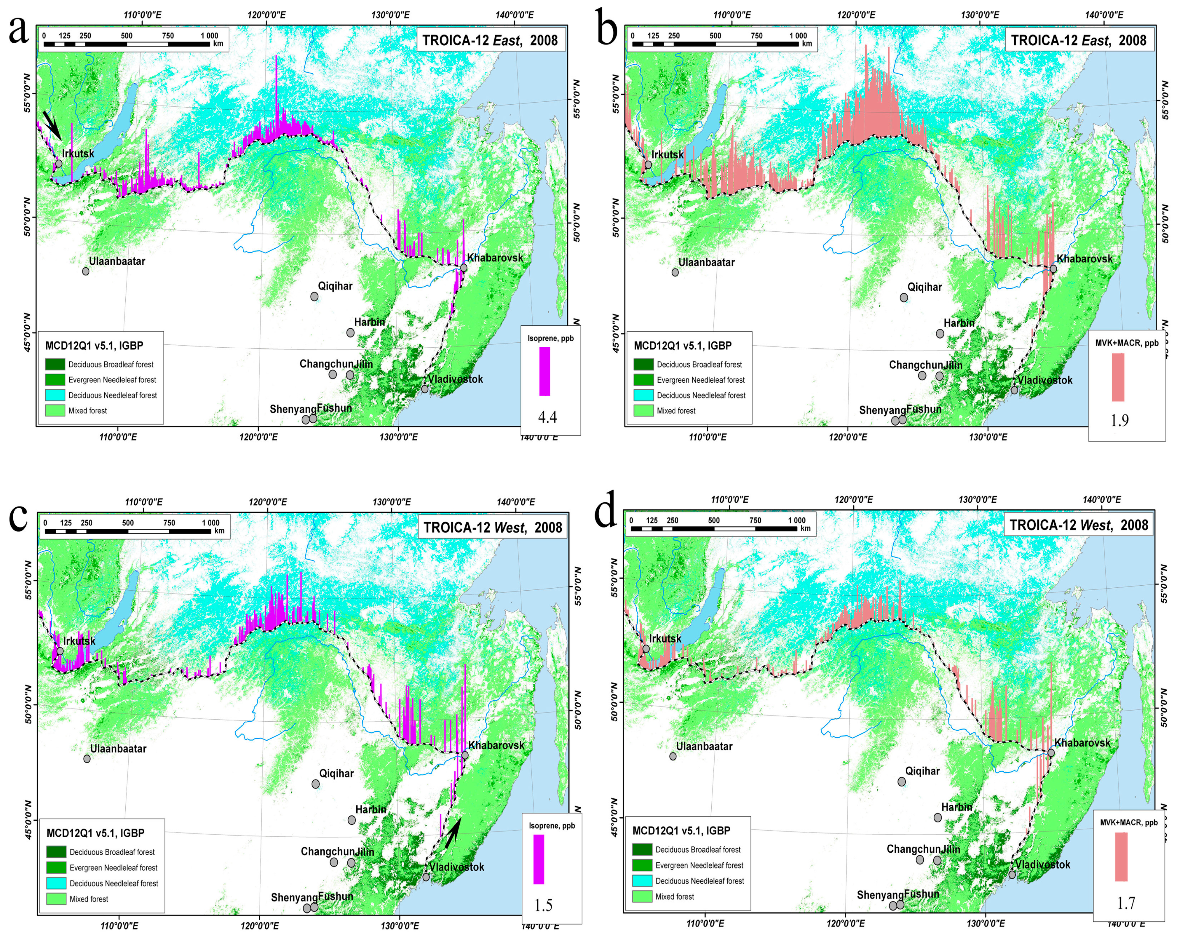
3.1. Spatial Distribution of Isoprene in the Far East Region from the TROICA-12 Experiment

The spatial distributions of isoprene and MVK+MACR concentrations in the Far East region, along the Trans-Siberian Railway of the TROICA-12 measurements (East and West routes), are presented in Figure 1 using of the ARC Info GIS system (computer cartography). The satellite MODIS vegetation map: MCD12Q1 v5.1, IGBP (2007) of broadleaf, needleaf and mixed forest, with a 500-m spatial resolution, was used as a marker of forest distribution in this region.
High concentrations of isoprene, along the route up to 5 ppb, correspond to biogenic emissions at noon. Note that the distribution of the MCD12Q1 land cover (Figure 1) and the MEGAN 2.04 land cover are slightly different. A more detailed discussion of the influence of LAI and PFT parameters on isoprene emissions, calculated using different vegetation maps, can be found in the study of Reference [8]. A comparison of different vegetation maps was also previously discussed in the study of Reference [51].
It should be noted that the TROICA-12 East isoprene concentration in the Far East region was 0.2 ppb higher, on average, than that of the TROICA-12 West, which might be caused by the temperature being 4°C higher in the TROICA East and by the different wind directions in these experiments.

3.2. The Comparison of Experimental Data with Isoprene mModel Calculations

Conditionally, the chemical reactions of isoprene oxidation can generally be divided into daytime (the reactions with O3 and OH) and night-time (the reactions with NO3 and O3) reactions. Note that NO3 is mainly produced in the industrial plumes and in an urban atmosphere at night. Therefore, in unpolluted areas, night-time isoprene sinks down into the residual ozone, which was produced during the daytime due to the photolysis reaction. The biogenic VOC lifetimes for daytime and night-time conditions are calculated and presented in Table 2. The corresponding reaction rates for OH, NO3 and O3 reactions at 298 K are shown in Table S1. The isoprene lifetime in the daytime is equal to ~1.24 h and to ~1.52 h at night-time, in the presence of 40 pptv NO3.
Thus, at the isoprene lifetime of ~1 h and at the wind speed of ~3–5 m·s−1, observed in the experiment, the forest massif, located about 10–20 km from the Trans-Siberian Railway, will influence the isoprene chemistry.
We compared the isoprene measurements with the simulations of the regional WRF-CHEM and global GEOS-CHEM models for TROICA-12 East and West (Figure 3a,b). The WRF-CHEM and GEOS-CHEM simulations of isoprene concentrations are in good agreement with the 10-min average data from TROICA-12. Thus, by comparing the green and blue curves, we can see, in Figure 3 (see also Figure 4 below), that the simulation results for the isoprene distribution depend more on the applied vegetation maps than on the chemical gas-phase mechanisms. This is not surprising, as the isoprene lifetime in the daytime is equal to ~1.24 h and at night-time it is equal to 1.52 h (Table 2). Thus, the advection, convection patterns, cloud distribution, radiation, as well as differences in the chemical mechanism weakly affected the spatial isoprene distribution.

3.3. The Comparison of Isoprene Concentration Fields Simulated by Different Models

In this section, the isoprene concentration fields were simulated and compared by WRF-CHEM and GEOS-CHEM models. As an example, the spatial distributions of isoprene at 26.07.2008 12 UTC, calculated by the RACM-MIM, MOZART gas-phase mechanism of WRF-CHEM and by GEOS-CHEM are shown on Figure 4a, Figure 4b and Figure 4c, respectively. A comparison of the external simulation, obtained by the MOZART-4 model, with the fields of GEOS-5 (Figure 4d) was also performed.
As already mentioned above, it is clear from Figure 4 that the spatial distribution of isoprene depends more on the vegetation covered land than on the chemical processes in the atmosphere modelling. Herewith, the MOZART-4 model gives more than 3.0 ppb in the extended area in comparison with WRF-CHEM and GEOS-CHEM models (Figure 4d). This is likely due to the fact that MOZART-4 model uses a coarse vegetation map.
All the model simulations were in good agreement with the experimental data for isoprene. Thus, we confirm that the biogenic emission model MEGAN can be used for a wide range of canopies.

4. The Secondary Isoprene Oxidation Reactions

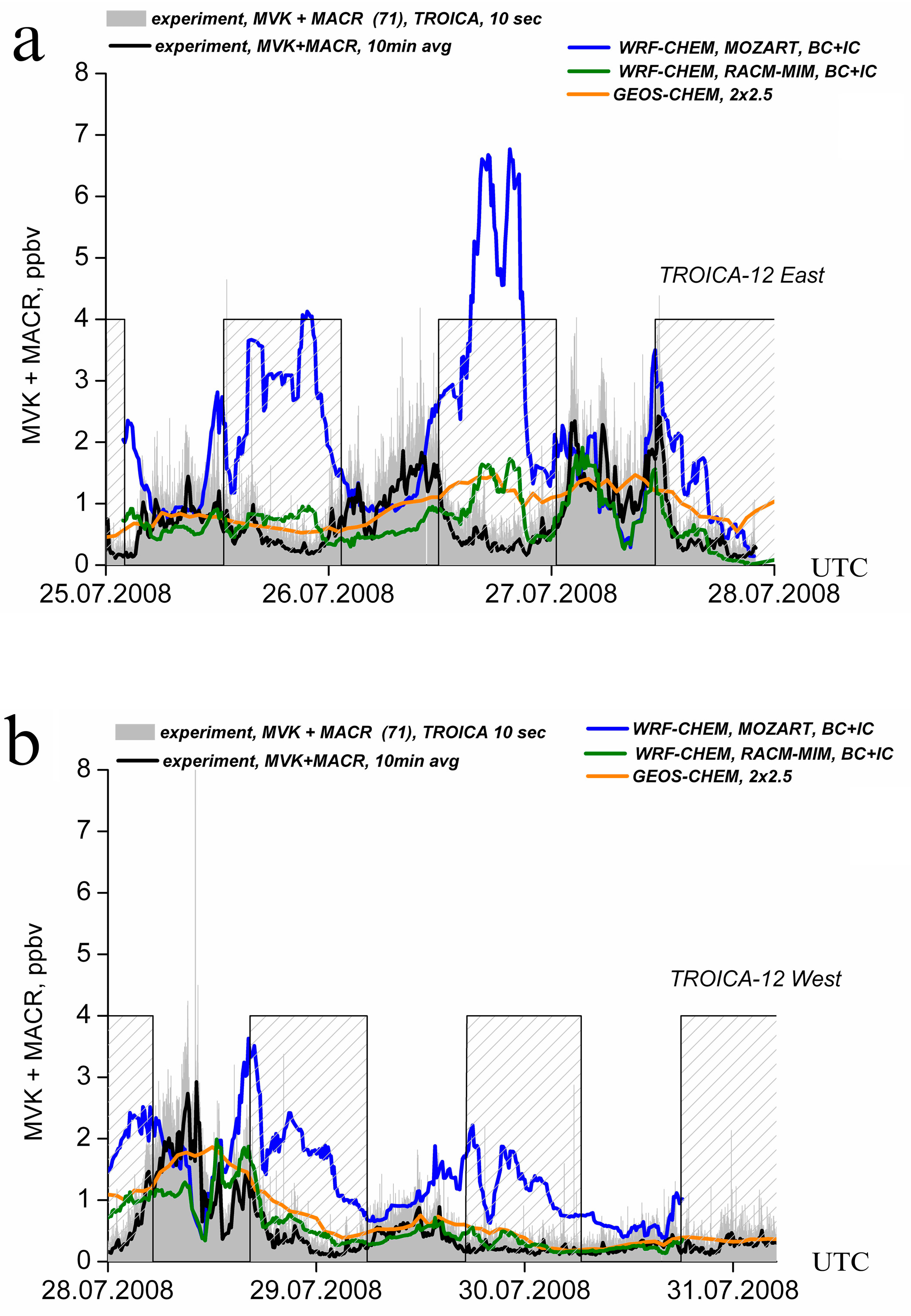
4.1. The Comparison Between the Experimental Data and the Results of the Model Simulation for the Secondary Isoprene Oxidation Products

Like isoprene oxidation, the MVK and MACR oxidation is caused by the reactions with OH and O3 in the daytime and by the reactions of MVK and MACR with NO3 and O3 at night. The MVK + MACR measurements were compared with the simulations of the regional WRF-CHEM and global GEOS-CHEM models for TROICA-12 East and West (see Figure 5).
The areas corresponding to nocturnal measurements are shaded in Figure 5. According to the model simulations, presented in Figure 5a,b, the nocturnal accumulations of MVK and MACR should be observed. Thus, the MOZART gas-phase mechanism of the WRF-CHEM model predicts a substantial growth of the sum of MVK and MACR concentrations in a range of ~2–7 ppb. Two other mechanisms, also at night, predict an increase in the MVK + MACR concentrations but a negligible one. These simulated values are in a range of ~0.5–1.5 ppb. The nocturnal accumulations of MVK and MACR is not surprising, as at night, the MVK and MACR reactions are suppressed and the MVK and MACR lifetimes are long in comparison to daytime lifetimes and are equal to 58.98 and 141.36 h (see Table 2).
At night, none of the models used provide any agreement with the experimental measurements. The nocturnal accumulation of MVK and MACR, predicted by all models under low-NOx conditions, was not observed. On the other hand, at noon, the agreement between the model simulations for MVK + MACR concentrations should be considered to be satisfactory, that is, in contrast to the in-field validation, the cross-model validation passed.

4.2. The Diurnal Variation of the Experimental Ratio

For simplicity of discussion, the ratio obtained from the experimental values below was called the “experimental ratio.” The experimental ratio was present in Figure 6, together with the result from the model simulations.
First, the average MVK+MACR-to-isoprene ratio (ratio), obtained from experimental data, does not have a clear diurnal cycle (Figure 6). Additionally, it should be noted that the daytime isoprene chemistry was in good agreement only for the oldest RACM-MIM model (2000). The GEOS-CHEM model with the modernized CIS isoprene block (2012) showed a result that is similar to the RACM-MIM scheme result in the first half of the day and to the MOZART scheme result in the second half of the day.

4.3. The Experimental Ratio from Twilight–Nighttime

The dependence of MVK + MACR on isoprene in the twilight–night-time period, from 21 to 24 LT (0.875–1.0), with no data separation by NOx levels (Figure 7), shows that, from 21 to 22 LT, the decrease of MVK and MACR is possibly suppressed due to the elimination of the daily chemical reactions with OH and O3, although the isoprene emission from vegetation remains. This is especially clear for the TROICA-12 West (the orange points in Figure 7f). Furthermore, the regression line between the pair, MVK + MACR and isoprene is located below the 1:1 line (the red line in Figure 7c,f), although in theory, the regression line should pass above the 1:1 line.
The good correlation between MVK+MACR and isoprene was observed (Figure 7b,e). The correlations (R) are equal to 0.68 and 0.79 for TROICA-12 East and West, respectively. The slopes (B), presented in Figure 7b,e, tend to 1 and are equal to 0.93 and 1.04 for TROICA-12 East and West, correspondingly. Therefore, the 10-s measurements are uniformly distributed and do not disintegrated into separate areas, corresponding to night-time and daytime chemical reactions.
However, from twilight–night-time, the noise of the NO3-pathway (ratio > 10) and O3-pathway (ratio ~ 4–10) are very appreciable. The twilight–night-time noise of the experimental ratio values is mentioned in Reference [52] and [53].
Further, we will consider the diurnal variation of the simulated ratio.

4.4. The Diurnal Variation of the Simulated Ratio

The diurnal variations of the ratio calculated using the RACM-MIM and MOZART gas-phase mechanisms of WRF-CHEM model as well as the GEOS-CHEM 2° × 2.5° model, are shown in Figure 8.
For the RACM-MIM scheme, the correlation coefficients (R), slopes (B), standard deviations (SD) are equal to R = 0.5264; B = 1.1671; SD = 0.4605 for TROICA-12 East and are equal to R = 0.811; B = 1.1439; SD = 0.3221 for TROICA-12 West. The night-time isoprene oxidation reactions are noticeable but not strongly dominant (see grey points in Figure 8b,d). The ratio at night is about 5, on average but in the night hours, it can reach high values (10–50), especially in TROICA-12 East, since the presence of a long-range pollutant transport from the central industrial part of China took place. Thus, the high values of the night ratio can correspond to the night reactions of isoprene with anthropogenic NO3 (Figure 8a, ratio > 10). The ratios in the range of 4–10 correspond to the O3 pathway.
The results of the MOZART simulation show that the MOZART gas-phase mechanism, as opposed to the experiment, gives a large number of night points, with high values of ~10–50 (00:00–07:00 and 21:00–24:00 LT) (Figure 8e,g), wherein there are almost no points with values less than 5. The model simulations clearly show that all isoprene chemical processes break up the daytime and night-time ones. The grey dots in Fig10fh represent the night-time reactions and the green dots represent the daytime reactions. Due to this separation of the chemical processes, no correlation between the simulated MVK + MACR and isoprene was observed. Unlike the RACM-MIM scheme (Figure 8b,d), all points in the MOZART scheme (Figure 8f,h) are above the 1:1 line.
The GEOS-CHEM 2° × 2.5° simulation is in good agreement with the WRF-CHEM one but at night, it has a poor agreement with the experimental data as well (Figure 8i). At night, the ratio reaches values of ~30–50. Almost all simulated points in Figure 8j are above the 1:1 line, with B=1.78 and R=0.82. Thus, the slopes for MVK + MACR versus isoprene in the model simulations are somewhat higher than the slopes calculated from the measurements (Figure 7b,e).
Such a divergence between the simulated results and experimental data is a serious alarm signal. Comparing Figure 9b,e with the right column in Figure 10, it can be seen that, statistically, it is impossible to allocate neither the NO3-pathway, nor the O3-pathway. Generally speaking, the problem of a significant discrepancy between nocturnal model simulations and in-field measurements in the isoprene chemistry is not a new and an unexpected event. In some studies [54,55], the nocturnal values of the ratio are completely left out, while authors casually remarked that in the morning and during twilight, there was a discrepancy between the theory and experiments.

5. The Maps of Chemical Reactions

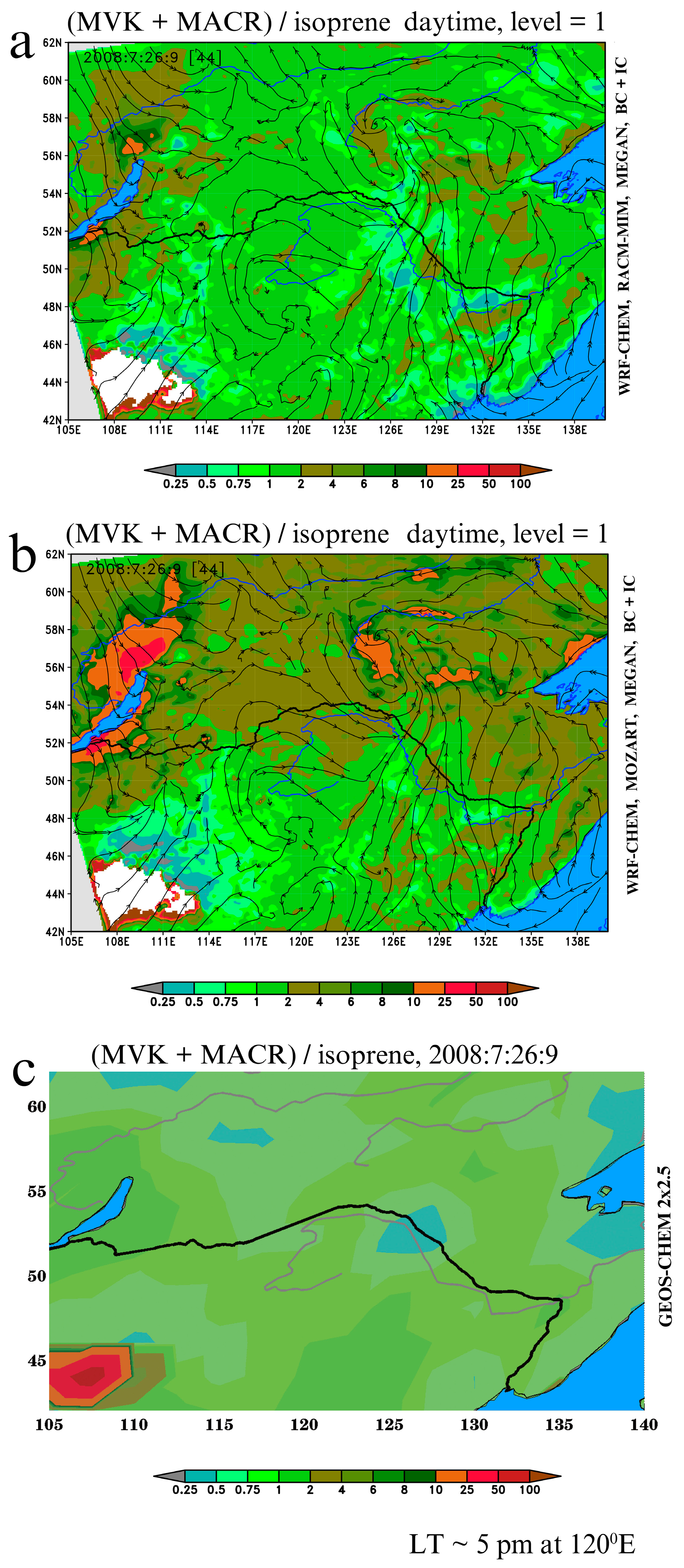
5.1. The Spatial Distribution of the Daytime Simulated Ratio

The spatial distribution of the ratio in the daytime is presented for RACM-MIM (Figure 9a) and MOZART (Figure 9b) gas-phase mechanisms and for the Caltech Isoprene Mechanism (CIS) of the GEOS-CHEM model, as exemplified by the distribution at 26.07.2008 09:00 UTC (~5 pm LT at 120° E longitude). The white areas in Figure 9 correspond to isoprene absence. Therefore, the ratio in these areas tends to be infinity. As a whole, the simulated spatial distribution of the daytime ratio is in a satisfactory agreement with the 10-min experimental data.

5.2. The Spatial Distribution of the Nocturnal Simulated Ratio

Similar to the daytime, at night, the spatial distributions of the ratio for RACM-MIM (Figure 10a), MOZART (Figure 10c) gas phase mechanisms and the Caltech Isoprene Mechanism (CIS) of the GEOS-CHEM model (Figure 10e) are presented for 18:00 UTC or ~2 a.m. LT at 120˚ E longitude. At night, under the low-NOx conditions along the Trans-Siberian Railway, isoprene reacts mainly with ozone. However, the rates of the MVK and MACR reactions with ozone are low and the corresponding lifetimes are equal to ~61 and 244 h, (Table 2). In this respect, it is not surprising that the RACM-MIM, MOZART and CIS mechanisms show high ratio values (up to 100).
Furthermore, the spatial distribution of NO3, one of the main night-time isoprene decreases, presented in Figure 10c,d, shows that the NO3 plume from the central regions of China reaches the Trans-Siberian Railway only in the case of modelling by the MOZART scheme. To the north of the Trans-Siberian Railway, differences in the spatial distribution of the ratio occur due to the differences in the ozone distribution, as a consequence of which isoprene decreases in the absence of NO3. The white areas in Figure 10a,c correspond to the areas where isoprene decreases completely on the NO3 plumes, as shown in Figure 10b,d.

6. Discussion

As was shown above, at night in large areas, the high ratio values should be observed (see Figure 10). It is of interest to find the answer to the question: did anyone observe such high ratio values at night and if such values were observed, under what conditions? It is absolutely clear that, if the corresponding high ratio has not been previously observed in in-field experiments, then there is a doubt in the correctness of the model chemical reactions used in CTM models, described in Reference [40,41,50].
According to independent studies [53,54,55,56,57,58,59,60,61,62], in which different devices and methods were used, the night-time ratio generally did not exceed 10 (in range of ~0.2–10), except in Reference [63].
In particular, according to Biesenthal et al. [56], at night, the average hourly values of the ratio do not exceed the values of 1.5–4.5, while initially, none of the averaged values of the ratio can reach ~5.0–5.5. In Reference [57], it was reported that the average hourly values do not exceed 2, while some initial values of the ratio reached ~7–8. The authors of Montzka et al. [58] paid attention to the significant discrepancies between the measurements and model results due to inaccurate simulation of the boundary layer dynamics by the model. The values of the ratio (32, 20 and 9.5) were reported by Reissell and Arey, in Reference [63], in the outflow at Pine Mountain from 20:00–24:00, when the night-time NO3 chemistry influenced the isoprene but not in the OH radical reaction. However, in most cases, the night-time ratio did not exceed 5.42 (August 5, 1997, 06:00–09:00 LT). Additionally, Cheung et al. [54] also reported high values of the ratio ~ 6 in several measurements at 7 a.m., 5 p.m. and 9 p.m. LT.
According to Langford et al., [59], the night-time ratio was less than 0.36 during the two intensive OP3 field campaigns (Oxidant and Particle Photochemical Processes above a South-East Asian Rainforest), which took place between 20 April–7 May, 20 June and 20 July 2008. The authors of Kalogridis et al., in Reference [60], reported that the ratio did not exceed 1.4 in a French Mediterranean oak forest. Night flights in the New England Air Quality Study (NEAQS) 2004 showed that the ratio was lower than 2.5 before sunset (see Table 2 in Reference [61]). Doughty et al. [53] wrote that it was expected that the ratio would increase to the daytime value of 0.16, since isoprene was no longer being emitted but was still being oxidized by O3. Indeed, they note that the night-time value was 0.21. The authors reported that, during the night, a signal to noise ratio was equal to ~3 and so they focused only on the first few night-time hours. Kaiser et al., in Reference [62], wrote that the night-time ratio was low and equal to ~0.3 at 20:00 LT and ~0.4 at 00:00 LT. Steinbacher et al., in Reference [64], indicate that the ratio has no diurnal variation and varied throughout the day from 0.4 to 0.9.
All of this testifies more likely in favour of the correctness of our measurements, than in favour of the model simulations, which predicted extremely high ratio values at night (Figure 8 and Figure 10). Therefore, it is more likely to indicate an error in the model schemes or in the fundamental principles of the chemical-transport modelling.
In this study, we used several model schemes [40,41,50]. The difference among the results that were obtained by these models is much less significant than the difference between the theoretical and experimental data. Therefore, the problem, described above, is determined not by the model chemical blocks that were used themselves but it is determined by the fundamental principle that is inherent in all CTM models. We must find an answer to the following question: What is the reason for the significant discrepancies between the theoretical and experimental data in the nocturnal time and during twilight?
Note that the theory in atmospheric chemistry is based on the results of the chemical kinetic measurements in the laboratory chambers (flasks) and on the subsequent computer simulations. As is well-known, the results of laboratory chemistry are extrapolated to the chemistry of the whole atmosphere. Furthermore, the most modern CTM models are a synthesis of the chemical Box Model, with a homogeneous distribution of all chemical species and the advections of the air masses (Chemistry + Transportation Model). Thus, the CTM models do not, in principle, have a mechanism that allows the heterogeneous processes in the gas-phase to be described. When we use CTM models, the homogeneity of the atmospheric structure as per the size of a domain cell is assumed. In our case, the domain has a horizontal resolution, which is equal to 18 × 18 km. Surely, some gases involved in the isoprene oxidation, such as OH, O3, are distributed almost homogeneously within the domain cell (Figure 11a). However, it is impossible to consider the homogeneous distribution of anthropogenic pollution from point sources. Furthermore, at the 18-km scale, a distribution of biogenic emissions is non-uniform due to heterogeneity of the massive forest (Figure 11b).
Heterogeneity in the gases’ distribution leads to the dependence of chemical reactions products from atmospheric mixing. The minimum atmospheric mixing height is observed at night, when the surface temperature inversion is set. At night, the dimension of heterogeneity is equal to 200–500 m. In the presence of competing chemical reactions, a switching from one reaction to another, depending on what compound is locally prevalent in a part of the cell, will take place. Especially, this effect appeared during twilight and the nocturnal hours, when the isoprene reactions with NO3 and O3 have rather different rates (see Table 2). When the atmospheric mixing is weak, the homogeneity of the chemical compounds’ distribution is reduced. During twilight, the system passes to the quasi-homogeneous state and then in inverted conditions, it passes to a heterogeneous state, in which the local species at a scale of ~200–500 m will significantly dominate over the background values.
For clarity, the processes considered in the Chemistry Science, Box Chemistry Models (BCM) and Chemical Transport Model (CTM) are included in Table 3. As can be seen from Table 3, in the transition from BCM to CTM, a big lacuna formed in theory due to the underestimation of the atmospheric mixing. The modern CTMs are based on only two chemical processes: a good mixing stage of homogeneous gas chemistry and a non-mixing stage of aerosol heterogeneous chemistry.
However, the real atmospheric chemistry consists of more than two processes. Additionally, it should be noted that the Secondary Organic Aerosol (SOA) is produced from the hydroxyl radical (OH)-initiated oxidation of isoprene (see Equations (S9)–(S11) in the Supplementary Materials). However, the SOA reactions concern the heterogenic aerosol chemistry section that is they are beyond the scope of our study. For more details about the SOA paths, please see the studies in Reference [65,66,67,68].
Therefore, we distinguish the quasi-heterogeneous gas chemistry and the heterogeneous gas chemistry. The Equations (S1)–(S11) that were used in this study, as well as all other ~ two hundred CTM chemical reactions (WRF-CHEM, GEOS-CHEM, etc.), were written under the homogenic chemistry condition. This view is not unique and unknown. Bridging the gap between atmospheric physics and chemistry in studies of small-scale turbulence is discussed in Reference [69].
The atmosphere mixing conditions can be described by the ratio, which was called the turbulent Damköhler number in Reference [70]:
D a S ( τ ) = τ m i x τ c h , S ;    τ m i x = h w * ;      τ c h , S = C S C s / t ;
where τ m i x is the mixing time scale of turbulence; h is the height of the planetary boundary layer; τ c h , S is the lifetime scale of the chemical species S, which depended on the concentration of the species S ( C S ) and the chemical rate for the species S ( C s / t ); and w * is the convective velocity scale, defined by Stull in Reference [71]:
w * = ( g h θ w θ ) 1 / 3
Note that the Damköhler numbers (turbulent Damköhler number and Kolmogorov Damköhler numbers) were used to determine the importance of the dynamics influence on chemistry in some studies, such as [53], [72,73,74,75,76,77,78,79,80,81,82,83,84].
Stockwell, in Reference [72], analysed reactions of a gas-phase chemical mechanism and found the reactions of OH (e.g., OH + NO2, OH + CO, OH + BVOC) and the reaction HO2 + NO to be diffusion-limited under typical turbulent atmospheric conditions or between diffusion limitation (τmix ~ τch) and kinetic regime (τmix >> τch) for the vertical transport under near-neutral to unstable conditions. Dlugi et al., in Reference [78], indicated that, for τmix << τch, the chemical constituents can be considered to be inert. However, for τmix >> τch, the species vary, as if driven by chemical kinetics or in chemical equilibrium. Later, in Reference [83], it was noted that comparing chemical simulations results, the homogeneously mixed reactants—especially in the case of bimolecular reactions—can have reaction rates that are significantly different from the well-mixed case.
According van Stratum et al. [81], based on the turbulent Damköhler number, the next regimes could be defined as: D a ( τ ) < 0.1 (slow chemistry), where the mixing ratio is controlled by the emission/deposition and ABL dynamics; 0.1 < D a ( τ ) < 10 (moderate chemistry), where the mixing ratio is governed by ABL dynamics and chemical reactions; and D a ( τ ) > 10 (fast chemistry), where the mixing ratio is determined by chemical reactions.
It should also be noted that authors in Reference [53] and [80] drew attention to the observed isoprene variability, which was greater than the instrumental noise, assuming Poissonian counting statistics [16] and they wrote that it likely occurred because isoprene was not well-mixed within the boundary layer in the afternoon. This is consistent with our isoprene observations in the daytime. If the convective velocity scale is 1 m s−1 and with our typical boundary layer depth of 1500 m, the boundary layer time scale would be ~0.42 h (see also Stull [71]). The lifetime of isoprene with an OH reaction is equal to 1.38 h, (Table 2). With these assumptions, the τ–Damköhler number for isoprene–OH is equal to 0.3. Thus, the heterogeneity is inherent not only in the spatial distribution of the secondary products, such as MVK and MACR in the nocturnal hours but some level of heterogeneity is inherent in the spatial distribution of isoprene due to the non-uniform distribution of vegetation near the measured complex and due to a weak mixing of the low troposphere.
In sum, most equations in WRF-CHEM and GEOS-CHEM are equitable under the condition of homogeneity. Therefore, any CTM chemistry models have some difficulties in forecasting VOC levels, especially at night-time (nocturnal time), including the models described in this study. CTM models should be provided with flags concerning the simulation quality (turbulent Damköhler number and Kolmogorov Damköhler numbers), without which any CTM simulations will be unreliable. Now, these CTM models are based on NCEP forecast systems. The maximum permissible concentrations of species are usually observed under conditions of poor atmospheric mixing, in particular, under night-time temperature inversions. The cost of the CTM forecast errors will be very high. In this situation, we cannot recommend that the CTM models use NCEP systems for forecasting, since any simulation CTM results beyond the Damköhler limits have the status of being hypothetical.

7. Conclusions

A detailed analysis of the spatial and temporal distributions of one of the main biogenic VOCs, isoprene and its oxidation products is presented in this study for the Far East region of Russia, along the Trans-Siberian Railway. The analysis was performed using the measurement data in TROICA experiments in a mobile laboratory and model simulations. It is shown that the measured temporal distribution of isoprene in the Far East region is in good agreement with the simulation of the WRF-CHEM and GEOS-CHEM models.
The simulated spatial isoprene distribution is more dependent on the applied vegetation maps than on the differences in the chemical algorithms. It was also shown that the measured isoprene, MVK and MACR have pronounced diurnal variations, while the average MVK + MACR-to-isoprene ratio (ratio) does not have a clear diurnal cycle. Moreover, the sum of MVK + MACR has a good correlation with isoprene (R ~ 0.60–0.86), while from the model calculations, the correlation between MVK + MACR and isoprene is almost absent and the distribution of points is broken up into night-time and daytime values. The simulated ratio, contrary to the experimental data, has pronounced diurnal variations. During twilight and the night-time, both the MOZART gas phase mechanism in the WRF CHEM model and the CIS isoprene mechanism in GEOS CHEM gave simulated ratio values of not less than 10. Such values were neither observed in our TROICA-12 expedition, nor in the literature referred to earlier.
In this study, we pointed to poor mixing as the most probable cause of the discrepancy between the theory and experiment at night and in the nocturnal hours. As for other reasons, it is possible to specify the failure of PTRMS due to the decomposition of ISOPOOH, the missed MVK and MACR decay reactions in the modern CTM, incorrect model parameters for the formation of SOA (second organic aerosol) or a decrease in MVK/MACR for the in-haze OH radical.
We propose that, because of the kinetic equations of CTM models are valid only in the homogeneous system, all chemical and transport (CTM) models, which are based on these kinetic equations, will not provide an adequate simulation in a poor mixed atmosphere at night. The atmospheric structure becomes heterogeneous during this time period. Thus, we recommend the use of the modern CTM in the tropical and equatorial zones. However, at moderate latitudes, we recommend the use of the CTM only in the warm period, at noon, when convective processes are guaranteed to ensure homogenic mixing conditions of species in the whole volume of the domain cell. These recommendations are given primarily for NCEP Services, where CTM models are used as a forecast system.

Supplementary Materials

The following are available online at https://www.mdpi.com/2073-4433/10/3/152/s1, S1: Basic chemical reactions of isoprene oxidation, S2: Secondary oxidation products of biogenic components, S3: Rate constants and lifetimes for biogenic VOCs.

Author Contributions

A.N.S. designed the study, analysed the data, conducted the WRF-CHEM model simulations and wrote the manuscript. Y.A.S. carried out the GEOS-CHEM model simulations. V.S.R. measured the anthropogenic pollutions in China and analysed the pollution transfer from China to the Trans-Siberian Railway. A.I.S. carried out the TROICA-12 expedition and analysed the data. E.V.B. participated in developing VOC emissions. I.B.B. implemented the mobile observatory experimental methods and measured the concentrations during the TROICA expeditions. N.F.E. headed the TROICA project and contributed to the study design and the discussion of the results.

Funding

The current research was supported by the Russian Foundation for Basic Research (Grant Nos. RFBR 17-29-05102 and RFBR 18-35-20031).

Conflicts of Interest

The authors declare no conflict of interest.

References

  1. Guenther, A.; Karl, T.; Harley, P.; Wiedinmyer, C.; Palmer, P.I.; Geron, C. Estimates of global terrestrial isoprene emissions using MEGAN (Model of Emissions of Gases and Aerosols from Nature). Atmos. Chem. Phys. 2006, 6, 3181–3210. [Google Scholar] [CrossRef] [Green Version]
  2. Warneke, C.; de Gouw, J.A.; Goldan, P.D.; Kuster, W.C.; Williams, E.J.; Lerner, B.M.; Jakoubek, R.; Brown, S.S.; Stark, H.; Aldener, M.; et al. Comparison of daytime and night-time oxidation of biogenic and anthropogenic VOCs along the New England coast in summer during New England Air Quality Study 2002. J. Geophys. Res. 2004, 109. [Google Scholar] [CrossRef]
  3. Crutzen, P.J.; Golitsyn, G.S.; Elansky, N.F.; Brenninkmeijer, C.A.M.; Scharffe, D.H.; Belikov, I.B.; Elokhov, A.S. Observations of minor impurities in the atmosphere over the Russian territory with the application of a railroad laboratory car. Dokl. Earth Sci. 1996, 351, 1289–1293. [Google Scholar]
  4. Crutzen, P.J.; Elansky, N.F.; Hahn, M.; Golitsyn, G.S.; Brenninkmeijer, C.A.M.; Scharffe, D.H.; Belikov, I.B.; Maiss, M.; Bergamaschi, P.; Röckmann, T.; et al. Trace Gas Measurements Between Moscow and Vladivostok Using the TransSiberian Railroad. J. Atmos. Chem. 1998, 29, 179–194. [Google Scholar] [CrossRef]
  5. Oberlander, E.A.; Brenninkmeijer, C.A.M.; Crutzen, P.J.; Elansky, N.F.; Golitsyn, G.S.; Granberg, I.G.; Scharffe, D.H.; Hofmann, R.; Belikov, I.B.; Paretzke, H.G.; et al. Trace gas measurements along the Trans-Siberian railroad: The TROICA 5 expedition. J. Geophys. Res. Atmos. 2002, 107. [Google Scholar] [CrossRef]
  6. Timkovsky, I.; Elanskii, N.F.; Skorokhod, A.I.; Shumskii, R.A. Studying of biogenic volatile organic compounds in the atmosphere over Russia. Izv. Atmos. Ocean. Phys. 2010, 46, 319–327. [Google Scholar] [CrossRef]
  7. Skorokhod, A.I.; Berezina, E.V.; Moiseenko, K.B.; Elansky, N.F.; Belikov, I.B. Benzene and toluene in the surface air of northern Eurasia from TROICA-12 campaign along the Trans-Siberian Railway. Atmos. Chem. Phys. 2017, 17, 5501–5514. [Google Scholar] [CrossRef] [Green Version]
  8. Guenther, A.B.; Jiang, X.; Heald, C.L.; Sakulyanontvittaya, T.; Duhl, T.; Emmons, L.K.; Wang, X. The Model of Emissions of Gases and Aerosols from Nature version 2.1 (MEGAN2.1): An extended and updated framework for modelling biogenic emissions. Geosci. Model Dev. 2012, 5, 1471–1492. [Google Scholar] [CrossRef]
  9. Atkinson, R. Gas-phase tropospheric chemistry of organic compounds. J. Phys. Chem. Ref. Data Monogr. 1994, 2, 1–216. [Google Scholar]
  10. Elansky, N.F.; Belikov, I.B.; Berezina, E.V.; Brenninkmeijer, C.A.M.; Buklikova, N.N.; Crutzen, P.J.; Elansky, S.N.; Elkins, J.V.; Elokhov, A.S.; Golitsyn, G.S.; et al. Atmospheric Composition Observations over Northern Eurasia Using the Mobile Laboratory: TROICA Expedition; Agrospas: Moscow, Russia, 2009; 76p, Available online: http://ifaran.ru/troica/biblio/troica-en.pdf (accessed on 31 January 2019).
  11. Panin, L.V.; Elansky, N.F.; Belikov, I.B.; Granberg, I.G.; Andronova, A.V.; Obvintsev, Y.I.; Bogdanov, V.M.; Grisenko, A.M.; Mozgrin, V.S. Estimation of Reliability of the Data on Pollutant Content Measured in the Atmospheric Surface Layer in the TROICA Experiments. Izv. Atmos. Ocean. Phys. 2001, 37, 81–91. [Google Scholar]
  12. Marais, E.A.; Jacob, D.J.; Jimenez, J.L.; Campuzano-Jost, P.; Day, D.A.; Hu, W.; Krechmer, J.; Zhu, L.; Kim, P.S.; Miller, C.C.; et al. Aqueous-phase mechanism for secondary organic aerosol formation from isoprene: Application to the southeast United States and co-benefit of SO2 emission controls. Atmos. Chem. Phys. 2016, 16, 1603–1618. [Google Scholar] [CrossRef]
  13. Rivera-Rios, J.C.; Nguyen, T.B.; Crounse, J.D.; Jud, W.; St. Clair, J.M.; Mikoviny, T.; Gilman, J.B.; Lerner, B.M.; Kaiser, J.B.; de Gouw, J.; et al. Conversion of hydroperoxides to carbonyls in field and laboratory instrumentation: Observational bias in diagnosing pristine versus anthropogenically controlled atmospheric chemistry. Geophys. Res. Lett. 2014, 41, 8645–8651. [Google Scholar] [CrossRef] [Green Version]
  14. Lindinger, W.; Hansel, A.; Jordan, A. Proton-transfer-reaction mass spectrometry (PTR-MS): On-line monitoring of volatile organic compounds at pptv levels. Chem. Soc. Rev. 1998, 27, 347–354. [Google Scholar] [CrossRef]
  15. Hewitt, C.N.; Haywardaand, S.; Tani, A. The application of proton transfer reaction-mass spectrometry (PTR-MS) to the monitoring and analysis of volatile organic compounds in the atmosphere. J. Environ. Monit. 2003, 5, 1–7. [Google Scholar] [CrossRef]
  16. De Gouw, J.; Warneke, C. Measurements of volatile organic compounds in the earth’s atmosphere using proton-transfer-reaction mass spectrometry. Mass Spectrom. Rev. 2007, 26, 223–257. [Google Scholar] [CrossRef]
  17. Blake, R.S.; Monks, P.S.; Ellis, A.M. Proton-Transfer Reaction Mass Spectrometry. Chem. Rev. 2009, 109, 861–896. [Google Scholar] [CrossRef]
  18. Yokelson, R.J.; Karl, T.; Artaxo, P.; Blake, D.R.; Christian, T.J.; Griffith, D.W.T.; Guenther, A.; Hao, W.M. The Tropical Forest and Fire Emissions Experiment: Overview and airborne fire emission factor measurements. Atmos. Chem. Phys. 2007, 7, 5175–5196. [Google Scholar] [CrossRef]
  19. Brenninkmeijer, C.A.M.; Crutzen, P.; Boumard, F.; Dauer, T.; Dix, B.; Ebinghaus, R.; Filippi, D.; Fischer, H.; Franke, H.; Frieβ, U.; et al. Civil Aircraft for the regular investigation of the atmosphere based on an instrumented container: The new CARIBIC system. Atmos. Chem. Phys. 2007, 7, 4953–4976. [Google Scholar] [CrossRef] [Green Version]
  20. IONICON Analytik GmbH Product Description. Available online: http://www.ptrms.com (accessed on 31 January 2019).
  21. Warneke, C.; De Gouw, J.A.; Kuster, W.C.; Goldan, P.D.; Fall, R. Validation of atmospheric VOC measurements by proton-transfer-reaction mass spectrometry using a gaschromatographic preseparation method. Environ. Sci. Technol. 2003, 37, 2494–2501. [Google Scholar] [CrossRef]
  22. Baker, B.; Guenther, A.; Greenberg, J.; Goldstein, A.; Fall, R. Canopy fluxes of 2-methyl-3-buten-2-ol over a ponderosa pine forest by relaxed eddy accumulation: Field data and model comparison. J. Geophys. Res. Atmos. 1999, 104. [Google Scholar] [CrossRef]
  23. Schade, G.W.; Goldstein, A.H.; Gray, D.W.; Lerdau, M.T. Canopy and leaf level 2-methyl-3-buten-2-ol fluxes from a ponderosa pine plantation. Atmos. Environ. 2000, 34, 3535–3544. [Google Scholar] [CrossRef]
  24. Karl, T.; Hansel, A.; Cappellin, L.; Kaser, L.; Herdlinger-Blatt, I.; Jud, W. Selective measurements of isoprene and 2-methyl-3-buten-2-ol based on NO+ ionization mass spectrometry. Atmos. Chem. Phys. 2012, 12, 11877–11884. [Google Scholar] [CrossRef] [Green Version]
  25. Skamarock, W.C.; Klemp, J.B.; Dudhia, J.; Gill, D.O.; Barker, D.; Duda, M.G.; Huang, X.-Y.; Wang, W.; et al. A Description of the Advanced Research WRF Version 3; NCAR Technical Note NCAR/TN-475+STR; National Center for Atmospheric Research: Boulder, CO, USA, 2008; p. 113. [Google Scholar] [CrossRef]
  26. NCEP FNL DS083.2 Meteorological Fields, National Centers for Environmental Prediction/National Weather Service/NOAA/U.S. Department of Commerce. 2000, Updated Daily. NCEP FNL Operational Model Global Tropospheric Analyses, Continuing from July 1999. Research Data Archive at the National Center for Atmospheric Research, Computational and Information Systems Laboratory. Available online: http://rda.ucar.edu/datasets (accessed on 31 January 2019).
  27. Grell, G.A.; Devenyi, D. A generalized approach to parameterizing convection combining ensemble and data assimilation techniques. Geophys. Res. Lett. 2002, 29. [Google Scholar] [CrossRef]
  28. Jiménez, P.A.; Dudhia, J.; González-Rouco, J.F.; Navarro, J.; Montávez, J.P.; García-Bustamante, E. A Revised Scheme for the WRF Surface Layer Formulation. Mon. Weather Rev. 2012, 140, 898–918. [Google Scholar] [CrossRef] [Green Version]
  29. Hong, S.-Y.; Noh, Y.; Dudhia, J. A New Vertical Diffusion Package with an Explicit Treatment of Entrainment Processes. Mon. Weather Rev. 2006, 134, 2318–2341. [Google Scholar] [CrossRef] [Green Version]
  30. Chen, F.; Mitchell, K.; Schaake, J.; Xue, Y.; Pan, H.-L.; Koren, V.; Duan, Q.Y.; Ek, M.; Betts, A. Modeling of land-surface evaporation by four schemes and comparison with FIFE observations. J. Geophys. Res. 1996, 101, 7251–7268. [Google Scholar] [CrossRef]
  31. Koren, V.; Schaake, J.; Mitchell, K.; Duan, Q.-Y.; Chen, F.; Baker, J.M. A parameterization of snowpack and frozen ground intended for NCEP weather and climate models. J. Geophys. Res. 1999, 104, 19569–19585. [Google Scholar] [CrossRef] [Green Version]
  32. Chou, M.-D. Parameterization for the absorption of solar radiation by O2 and CO2 with application to climate studies. J. Clim. Appl. Meteorol. 1990, 3, 209–217. [Google Scholar] [CrossRef]
  33. Chou, M.-D. A solar radiation model for climate studies. J. Atmos. Sci. 1992, 49, 762–772. [Google Scholar] [CrossRef]
  34. Chou, M.D.; Suarez, M.J. An Efficient Thermal Infrared Radiation Parameterization for Use in General Circulation Models; NASA Technical Memorandum 104606; National Aeronautics and Space Administration: Greenbelt, MD, USA, 1994; Volume 3, p. 85.
  35. Mlawer, E.J.; Taubman, S.J.; Brown, P.D.; Iacono, M.J.; Clough, S.A. Radiative transfer for inhomogeneous atmospheres: RRTM, a validated correlated-k model for the longwave. J. Geophys. Res. 1997, 102, 16663–16682. [Google Scholar] [CrossRef] [Green Version]
  36. Lin, Y.-L.; Farley, R.D.; Orville, H.D. Bulk Parameterization of the Snow Field in a Cloud Model. J. Clim. Appl. Meteorol. 1983, 22, 1065–1092. [Google Scholar] [CrossRef] [Green Version]
  37. Wicker, L.J.; Skamarock, W.C. Time-splitting methods for elastic models using forward time schemes. Mon. Weather Rev. 2002, 130, 2088–2097. [Google Scholar] [CrossRef]
  38. Skamarock, W.C. Positive-Definite and Monotonic Limiters for Unrestricted-Timestep Transport Schemes. Mon. Weather Rev. 2006, 134, 2241–2250. [Google Scholar] [CrossRef]
  39. Smagorinsky, J. General circulation experiments with the primitive equations: 1. The basic experiment. Mon. Weather Rev. 1963, 91, 99–164. [Google Scholar] [CrossRef]
  40. Pöschl, U.; von Kuhlmann, R.; Poisson, N.; Crutzen, P.J. Development and Intercomparison of Condensed Isoprene Oxidation Mechanisms for Global Atmospheric Modeling. J. Atmos. Chem. 2000, 37, 29–52. [Google Scholar] [CrossRef]
  41. Emmons, L.K.; Walters, S.; Hess, P.G.; Lamarque, J.-F.; Pfister, G.G.; Fillmore, D.; Granier, C.; Guenther, A.; Kinnison, D.; Laepple, T.; et al. Description and evaluation of the Model for Ozone and Related chemical Tracers, version 4 (MOZART-4). Geosci. Model Dev. 2010, 3, 43–67. [Google Scholar] [CrossRef] [Green Version]
  42. Janssens-Maenhout, G.; Dentener, F.; van Aardenne, J.; Monni, S.; Pagliari, V.; Orlandini, L.; Klimont, Z.; Kurokawa, J.; Akimoto, H.; Ohara, T.; et al. EDGAR-HTAP: A harmonized gridded air pollution emission dataset based on national inventories. In JRC Scientific and Technical Reports; European Union: Luxembourg, 2012; p. 41. [Google Scholar]
  43. EDGAR-HTAP. Available online: http://edgar.jrc.ec.europa.eu/national_reported_data/htap.php (accessed on 31 January 2019).
  44. EDGAR v4.1, Dataset in the Global Emission Section. Available online: ftp://aftp.fsl.noaa.gov/divisions/taq/global_emissions/ (accessed on 31 January 2019).
  45. Guenther, A.; Hewitt, C.N.; Erickson, D.; Fall, R.; Geron, C.; Graedel, T.; Harley, P.; Klinger, L.; Lerdau, M.; Mckay, W.A.; et al. A global model of natural volatile organic compound emissions. J. Geophys. Res. 1995, 100, 8873–8892. [Google Scholar] [CrossRef]
  46. Guenther, A.; Baugh, B.; Brasseur, G.; Greenberg, J.; Harley, P.; Klinger, L.; Serca, D.; Vierling, L. Isoprene emission estimates and uncertainties for the Central African EXPRESSO study domain. J. Geophys. Res. 1999, 104, 30625–30639. [Google Scholar] [CrossRef]
  47. Guenther, A.; Jiang, X.; Duhl, T.; Sakulyanontvittaya, T.; Johnson, J.; Wang, X. User’s Guide to the MEGAN Version 2.10. Available online: Lar.wsu.edu/megan/docs/MEGAN2.1_User_GuideWSU.pdf (accessed on 31 January 2019).
  48. NCAR ACOM. Available online: https://www2.acom.ucar.edu/wrf-chem/wrf-chem-tools-community (accessed on 31 January 2019).
  49. GEOS-CHEM. Available online: http://acmg.seas.harvard.edu/geos/ (accessed on 31 January 2019).
  50. Paulot, F.; Henze, D.K.; Wennberg, P.O. Impact of the isoprene photochemical cascade on tropical ozone. Atmos. Chem. Phys. 2012, 12, 1307–1325. [Google Scholar] [CrossRef] [Green Version]
  51. Safronov, A.N.; Fokeeva, E.V.; Rakitin, V.S.; Yurganov, L.N.; Grechko, E.I. Carbon monoxide emissions in summer 2010 in the central part of the Russian Plain and estimation of their uncertainties with the use of different land-cover maps. Izv. Atmos. Ocean. Phys. 2012, 48, 925–940. [Google Scholar] [CrossRef]
  52. Baldocchi, D.; Guenther, A.; Harley, P.; Klinger, L.; Zimmerman, P.; Lamb, B.; Westberg, H. The fluxes and air chemistry of isoprene above a deciduous hardwood forest. Philos. Trans. Phys. Sci. Eng. 1995, 351, 279–296. [Google Scholar]
  53. Doughty, D.; Fuentes, J.D.; Sakai, R.; Hu, X.-M.; Sanchez, K. Nocturnal isoprene declines in a semi-urban environment. J. Atmos. Chem. 2015, 72, 215–234. [Google Scholar] [CrossRef]
  54. Cheung, K.; Guo, H.; Ou, J.M.; Simpson, I.J.; Barletta, B.; Meinardi, S.; Blake, D.R. Diurnal profiles of isoprene, methacrolein and methyl vinyl ketone at an urban site in Hong Kong. Atmos. Environ. 2014, 84, 323–331. [Google Scholar] [CrossRef]
  55. Xiong, F.; McAvey, K.M.; Pratt, K.A.; Groff, C.J.; Hostetler, M.A.; Lipton, M.A.; Starn, T.K.; Seeley, J.V.; Bertman, S.B.; Teng, A.P.; et al. Observation of isoprene hydroxynitrates in the southeastern United States and implications for the fate of NOx. Atmos. Chem. Phys. 2015, 15, 11257–11272. [Google Scholar] [CrossRef]
  56. Biesenthal, T.A.; Wu, Q.; Shepson, P.B.; Wiebe, H.A.; Anlauf, K.G.; Mackay, G.I. A study of relationships between isoprene, its oxidation products and ozone, in the lower fraser valley, BC. Atmos. Environ. 1997, 98, 2049–2058. [Google Scholar] [CrossRef]
  57. Biesenthal, T.A.; Bottenheim, J.W.; Shepson, P.B.; Li, S.-M.; Brickell, P.C. The chemistry of biogenic hydrocarbons at a rural site in eastern Canada. J. Geophys. Res. Atmos. 1998, 103, 25487–25498. [Google Scholar] [CrossRef] [Green Version]
  58. Montzka, S.A.; Trainer, M.; Goldan, P.D.; Kuster, W.C.; Fehsenfeld, F.C. Isoprene and its oxidation products, methyl vinyl ketone and methacrolein, in the rural troposphere. J. Geophys. Res. Atmos. 1993, 98, 1101–1111. [Google Scholar] [CrossRef] [Green Version]
  59. Langford, B.; Misztal, P.K.; Nemitz, E.; Davison, B.; Helfter, C.; Pugh, T.A.M.; MacKenzie, A.R.; Lim, S.F.; Hewitt, C.N. Fluxes and concentrations of volatile organic compounds from a South-East Asian tropical rainforest. Atmos. Chem. Phys. 2010, 10, 8391–8412. [Google Scholar] [CrossRef] [Green Version]
  60. Kalogridis, C.; Gros, V.; Sarda-Esteve, R.; Langford, B.; Loubet, B.; Bonsang, B.; Bonnaire, N.; Nemitz, E.; Genard, A.-C.; Boissard, C.; et al. Concentrations and fluxes of isoprene and oxygenated VOCs at a French Mediterranean oak forest. Atmos. Chem. Phys. 2014, 14, 10085–10102. [Google Scholar] [CrossRef] [Green Version]
  61. Brown, S.S.; deGouw, J.A.; Warneke, C.; Ryerson, T.B.; Dubé, W.P.; Atlas, E.; Weber, R.J.; Peltier, R.E.; Neuman, J.A.; Roberts, J.M.; et al. Nocturnal isoprene oxidation over the Northeast United States in summer and its impact on reactive nitrogen partitioning and secondary organic aerosol. Atmosp. Chem. Phys. 2009, 9, 3027–3042. [Google Scholar] [CrossRef] [Green Version]
  62. Kaiser, J.; Skog, K.M.; Baumann, K.; Bertman, S.B.; Brown, S.B.; Brune, W.H.; Crounse, J.D.; de Gouw, J.A.; Edgerton, E.S.; Feiner, P.A.; et al. Speciation of OH reactivity above the canopy of an isoprene-dominated forest. Atmos. Chem. Phys. 2016, 16, 9349–9359. [Google Scholar] [CrossRef] [Green Version]
  63. Reissell, A.; Arey, J. Biogenic volatile organic compounds at Azusa and elevated sites during the 1997 Southern California Ozone Study. J. Geophys. Res. 2001, 106, 1607–1621. [Google Scholar] [CrossRef] [Green Version]
  64. Steinbacher, M.; Dommen, J.; Ordonez, C.; Reimann, S.; Gruebler, F.C.; Staehelin, J.; Andreani-Aksoyoglu, S.; Prevot, A.S.H. Volatile Organic Compounds in the Po Basin. Part B: Biogenic VOCs. J. Atmos. Chem. 2005, 51, 293–315. [Google Scholar] [CrossRef]
  65. Lin, Y.-H.; Zhang, H.; Pye, H.O.T.; Zhang, Z.; Marth, W.J.; Park, S.; Arashiro, M.; Cui, T.; Budisulistiorini, S.H.; Sexton, K.G.; et al. Epoxide as a precursor to secondary organic aerosol formation from isoprene photooxidation in the presence of nitrogen oxides. Proc. Natl. Acad. Sci. USA 2013, 110, 6718–6723. [Google Scholar] [CrossRef] [PubMed] [Green Version]
  66. Lin, Y.-H.; Arashiro, M.; Martin, E.; Chen, Y.; Zhang, Z.; Sexton, K.G.; Gold, A.; Jaspers, I.; Fry, R.C.; Surratt, J.D. Isoprene-derived secondary organic aerosol induces the expression of oxidative stress response genes in human lung cells. Environ. Sci. Technol. Lett. 2016, 3, 250–254. [Google Scholar] [CrossRef]
  67. Jiang, H.; Jang, M. Dynamic Oxidative Potential of Atmospheric Organic Aerosol under Ambient Sunlight. Environ. Sci. Technol. 2018, 52, 7496–7504. [Google Scholar] [CrossRef] [PubMed]
  68. Tuet, W.Y.; Chen, Y.; Fok, S.; Champion, J.A.; Ng, N.L. Inflammatory responses to secondary organic aerosols (SOA) generated from biogenic and anthropogenic precursors. Atmos. Chem. Phys. 2017, 17, 11423–11440. [Google Scholar] [CrossRef] [Green Version]
  69. Vilà-Guerau de Arellano, J. Bridging the gap between atmospheric physics and chemistry in studies of small-scale turbulence. Bull. Am. Meteorol. Soc. 2003, 84, 51–56. [Google Scholar] [CrossRef]
  70. Damköhler, G. Influence of turbulence on the velocity flames in gas mixtures. Z. Elektrochem. 1940, 46, 601–626. [Google Scholar]
  71. Stull, R.B. An Introduction to Boundary Layer Meteorology; Kluwer Academic Publishers: Dortrecht, The Netherlands, 1988. [Google Scholar]
  72. Stockwell, W.R. Effects of Turbulence on Gas-Phase Atmospheric Chemistry: Calculation of the Relationship Between Time Scales for Diffusion and Chemical Reaction. Meteorol. Atmos. Phys. 1995, 57, 159–171. [Google Scholar] [CrossRef]
  73. Vilà-Guerau de Arellano, J.; Duynkerke, P.G.; Zeller, K.F. Atmospheric surface layer similarity theory applied to chemically reactive species. J. Geophys. Res. 1995, 100, 1397–1408. [Google Scholar] [CrossRef]
  74. Molemaker, M.J.; Vilà-Guerau de Arellano, J. Turbulent control of chemical reactions in the convective boundary layer. J. Atmos. Sci. 1998, 55, 568–579. [Google Scholar] [CrossRef]
  75. Verver, G.H.L.; van Dop, H.; Holtslag, A.A.M. Turbulent mixing and the chemical breakdown of isoprene in the atmospheric boundary layer. J. Geophys. Res. 2000, 105, 3983–4002. [Google Scholar] [CrossRef] [Green Version]
  76. Vinuesa, J.-F.; Vilà-Guerau de Arellano, J. Introducing effective reaction rates to account for the inefficient mixing of the convective boundary layer. Atmos. Environ. 2005, 39, 445–461. [Google Scholar] [CrossRef]
  77. Vilà-Guerau de Arellano, J.; Gioli, B.; Miglietta, F.; Jonker, H.; Baltink, H.; Hutjes, R.; Holtslag, A. Entrainment process of carbon dioxide in the atmospheric boundary layer. J. Geophys. Res. Atmos. 2004, 109. [Google Scholar] [CrossRef]
  78. Dlugi, R.; Berger, M.; Zelger, M.; Hofzumahaus, A.; Siese, M.; Holland, F.; Wisthaler, A.; Grabmer, W.; Hansel, A.; Koppmann, R.; et al. Turbulent exchange and segregation of HOx radicals and volatile organic compounds above a deciduous forest. Atmos. Chem. Phys. 2010, 10, 6215–6235. [Google Scholar] [CrossRef] [Green Version]
  79. Pugh, T.A.M.; MacKenzie, A.R.; Hewitt, C.N.; Langford, B.; Edwards, P.M.; Furneaux, K.L.; Heard, D.E.; Hopkins, J.R.; Jones, C.E.; Karunaharan, A.; et al. Simulating atmospheric composition over a South-East Asian tropical rainforest: Performance of a chemistry box model. Atmos. Chem. Phys. 2010, 10, 279–298. [Google Scholar] [CrossRef]
  80. Pugh, T.A.M.; MacKenzie, A.R.; Langford, B.; Nemitz, E.; Misztal, P.K.; Hewitt, C.N. The influence of small scale variations in isoprene concentrations on atmospheric chemistry over a tropical rainforest. Atmos. Chem. Phys. 2011, 11, 4121–4134. [Google Scholar] [CrossRef]
  81. van Stratum, B.J.H.; Vilà-Guerau de Arellano, J.; Ouwersloot, H.G.; van den Dries, K.; van Laar, T.W.; Martinez, M.; Lelieveld, J.; Diesch, J.-M.; Drewnick, F.; Fischer, H.; et al. Case study of the diurnal variability of chemically active species with respect to boundary layer dynamics during DOMINO. Atmos. Chem. Phys. 2012, 12, 5329–5341. [Google Scholar] [CrossRef] [Green Version]
  82. Karl, T.; Misztal, P.K.; Jonsson, H.H.; Shertz, S.; Goldstein, A.H.; Guenther, A.B. Airborne flux measurements of BVOCs above Californian oak forests: Experimental investigation of surface and entrainment fluxes, OH densities and Damkohler numbers. J. Atmos. Sci. 2013, 70, 3277–3287. [Google Scholar] [CrossRef]
  83. Dlugi, R.; Berger, M.; Zelger, M.; Hofzumahaus, A.; Rohrer, F.; Holland, F.; Lu, K.; Kramm, G. The balances of mixing ratios and segregation intensity: A case study from the field (ECHO 2003). Atmos. Chem. Phys. 2014, 14, 10333–10362. [Google Scholar] [CrossRef]
  84. Kaser, L.; Karl, T.; Yuan, B.; Mauldin III, R.L.; Cantrel, C.A.; Guenther, A.B.; Patton, E.G.; Weinheimer, A.J.; Knote, C.; Orlando, J.; et al. Chemistry-turbulence interactions and mesoscale variability influence the cleansing efficiency of the atmosphere. Geophys. Res. Lett. 2015, 42, 10894–10903. [Google Scholar] [CrossRef]
Figure 1. Spatial distribution of isoprene (a,c) and methyl vinyl ketone (MVK) + methacrolein (MACR) (b,d) along the Trans-Siberian Railway, measured in TROICA-12 East (a,b) and West (c,d) experiments in July 2008. The MCD12Q1 v5.1, IGBP vegetation map of deciduous broadleaf, needleaf and mixed forest, with a 500 m resolution, obtained from the satellite data MODIS Terra and Aqua, is used as a background map. The arrow notes show the direction of the mobile-laboratory movement.
Atmosphere 10 00152 g001
Figure 2. The 10-min averaged concentrations of NO, NOx, O3 and CO, measured during the expeditions of TROICA-12 East and West on the stretch of the Trans-Siberian Railway from Lake Baikal to the Pacific Ocean coast. The CO concentrations are shown as an indicator of the long-range pollution transport. The arrow specifies a site corresponding to the long-distance pollution transport from the central regions of China, recorded during the expedition, TROICA-12 West.
Atmosphere 10 00152 g002
Figure 3. The comparison of the 10-sec initial experimental isoprene data (light grey areas) and the 10-min averaged data (grey lines) from TROICA-12 East (a) and West (b) measurements, with the simulations using the RACM-MIM and MOZART gas-phase mechanisms of the regional WRF-CHEM model and the CIS mechanism of the global GEOS-CHEM 2° × 2.5° model.
Atmosphere 10 00152 g003
Figure 4. The result of model simulations of the isoprene spatial distribution using two mechanisms of the regional chemical-transportation WRF-CHEM model: RACM-MIM ((a), this study) and MOZART ((b), this study), using the global GEOS-CHEM model ((c), this study) and from independent research: MOZART-4 model with GEOS-5 meteorological fields ((d), external). In addition, the (u,v) streamlines at the surface level of WRF-ARW and GEOS-5 meteorological fields were presented in (a,b,d) to visualize the direction of species flows.
Atmosphere 10 00152 g004
Figure 5. The comparison of the 10-sec initial experimental MVK+MACR data (light grey areas) and the 10-min averaged data (grey lines) from TROICA-12 East (a) and West (b) measurements, with the simulations of the regional WRF-CHEM model with the RACM-MIM and MOZART gas-phase mechanism and the global GEOS-CHEM model. The shaded rectangles correspond to night-time measurements (21:00–09:00 LT).
Atmosphere 10 00152 g005
Figure 6. Average diurnal variations of the ratio of experimental TROICA-12 East (a) and West (b) data and for model simulations. The shaded area shows the nocturnal values. The oscillations of 10 points, adjacent to the average GEOS-CHEM curve, is the result of averaging over a coarse spatial grid of 2 × 2.5°. Coincidence between the theoretical and experimental values (black line) is observed only for the WRF-CHEM RACM-MIM model (green line) in the range of 11–19 o’clock of LT. Unrealistic nocturnal model values have been cut off and are not represented in the Figure.
Atmosphere 10 00152 g006
Figure 7. The diurnal variations of the ratio, obtained from TROICA-12 East and West measurements, are shown in (a,d). The linear regressions based on measurements along the Far-East stage of the railroad are presented in (b,e). The discussed problematical nocturnal linear regressions in the twilight were coloured in (c,f) in the range of 21:00–24:00 LT, with a 30-min step. The corresponding daytime fraction is equal to 0.875–1.0, (red–blue colour). Red lines correspond to linear regressions. The dashed lines correspond to the ratio of 1:1.
Atmosphere 10 00152 g007
Figure 8. The diurnal variation of the ratio simulated using RACM-MIM and MOZART gas-phase mechanisms of the WRF-CHEM model and the CIS mechanism of the GEOS-CHEM model; (a,e)—TROICA-12 East and (c,g)—TROICA-12 West. Due to a rough resolution grid of 2 × 2.5° of the GEOS-CHEM model, which leads to lower numbers of N = 340, the statistical analysis was based on a joint analysis for East and West stages. The linear regression between MVK+MACR and isoprene, with an additional colour daytime fraction of 0.0–1.0 (00:00–24:00 LT), is presented for illustrating nocturnal and daily isoprene chemistry; (b,f)—TROICA-12 East and (d,h)—TROICA-12 West. The red lines correspond to the linear regression. The dashed lines correspond to the 1:1 ratio.
Atmosphere 10 00152 g008
Figure 9. An example of the daytime chemical reaction maps of the ratio at 26.07.2008 09:00 UTC (~5 pm LT at 120 °E), simulated by RACM-MIM (a) and MOZART gas-phase mechanisms (b) of the regional WRF-CHEM model and using the global GEOS-CHEM 2 × 2.5° model (c). In regional simulations, the long-range transport from the central industrial districts of China is taken into account. The white areas correspond to the values of the ratio >> 100, where isoprene is missing. In addition, the (u,v) streamlines at the surface level of WRF-ARW meteorological fields were presented in (a,b) to visualize the direction of species flows.
Atmosphere 10 00152 g009
Figure 10. An example of the nocturnal chemical reaction maps of the ratio at 26.07.2008 18:00 UTC (~2 am LT next day at 120° E), simulated by RACM-MIM (a) and MOZART (c) gas-phase mechanisms of the WRF-CHEM model and using the global GEOS-CHEM 2 × 2.5˚ model (e). In the regional simulation, the long-range transport from the central industrial districts of China is taken into account. The white areas correspond to the values of the ratio >>100, where the isoprene is missing. Spatial distributions of NO3 concentrations, calculated by the RACM-MIM mechanism (b), MOZART mechanism (d) and GEOS-CHEM (f), are presented. In addition, the (u,v) streamlines at the surface level of WRF-ARW meteorological fields were presented in (ad) to visualize the direction of species flows.
Atmosphere 10 00152 g010
Figure 11. The simple diagram, showing the transition due to the deterioration of the atmospheric mixing, from the homogeneous chemical state in the daytime (a) to a heterogeneous state in the night-time (b). The ellipses show the chemical compounds, which cannot have been uniformly distributed on a model domain scale. In this study, the horizontal size of a domain cell is equal to 18 km. On the one hand, the O3 and OH-radical are nearly homogeneously distributed in the troposphere [see (a)]. The diagram explains the reason for the increase of chemical reaction noises at night.
Atmosphere 10 00152 g011
Table 1. The parameterizations of the WRF-ARW meteorological model used in this study.
ParameterScheme, (Main Features)Reference
Cumulus parameterizationGrell 3D scheme, improved version of Grell-Devenyi scheme(Grell and Devenyi, 2002) [27]
Surface layerRevised MM5 Monin-Obukhov scheme(Jiménez et al., 2012), [28]
Boundary layer schemeYonsei University non-local-K scheme(Hong et al., 2006), [29]
Land-surface modelunified Noah land-surface scheme with soil temperature and moisture in 4-layers(Chen et al., 1996),
(Koren et al., 1999), [30,31]
Shortwave radiationGoddard (4-stream discrete-ordinate scattering, 8 bands) with ozone from climatology(Chou, 1990),
(Chou, 1992),
(Chou and Suarez, 1994), [32,33,34]
Longwave radiationRRTM (Long-wave correlated-k 16 bands with cloud optical depth)(Mlawer et al., 1997), [35]
MicrophysicsLin (Purdue cloud model, Mixed-phase with graupel)(Lin et al., 1983), [36]
Advection schemeRK3 scheme(Wicker and Skamarock, 2002),
(Skamarock, 2006), [37,38]
Subgrid horizontal mixinghorizontal deformation(Smagorinsky, 1963), [39]
Table 2. Lifetimes during the daytime and night-time for biogenic volatile organic compounds (VOCs) at 298 K.
CompoundReaction Lifetimes Day/Night, HoursTotal Compound Lifetime, Hours
τOHτNO3τO3DayNight
Isoprene1.38/––/1.6312.40/21.701.241.52
Methyl vinyl ketone7.39/––/1851.8534.81/60.926.0958.98
Methacrolein4.15/––/336.70139.24/243.664.03141.36
1 Day: [OH] = 2.0x10⁶ molec. cm−3; [NO3] = 0; [O3] = 1.75x10¹² molec. cm−3 (~70 ppbv); Night: [OH] = 0; [NO3] = 2.5 × 10⁸ molec. cm−3 (~40 pptv); [O3] = 1.0 × 10¹² molec. cm−3 (~40 ppbv).
Table 3. The comparison of the processes considered in the Chemistry Science, Box Chemistry Models (BCM), Chemical Transport Model (CTM) and Real Atmospheric Chemistry.
ObjectProcessStageVolume/Size
Chemistry Science 1homogenic chemistry –
heterogenic chemistry
2common statement
Box Chemistry Modelshomogenic chemistry (good mixing) –
heterogenic chemistry (none-mixing)
2particular case;
flask or camera; ~litres
Atmospheric mixinggood mixing (noon) –
half mixing (morning/evening) –
weakly mixing (nocturnal)
3In the daytime – convective cell; PBL ~ 4 km.
At night – height of nocturnal temperature inversion; ~200–600 m.
modern CTM modelsgas chemistry (good mixing, homogenic chemistry) –
aerosol chemistry (none-mixing, heterogenic chemistry)
2domain cell:
gas ~10 km in lat–lon scale;
aerosol – μm scale
Real Atmospheric Chemistry 2good mixing, (homogenic gas chemistry) –
half mixing, (quasi-heterogenic gas chemistry) –
non-mixing, (heterogenic gas chemistry and heterogenic aerosol chemistry)
3Stockwell limits in CTM modelling
1 – with some Criegee intermediate (CI) reactions, located between homogenic chemistry and heterogenic chemistry. 2 – the discussed statements were highlighted by bold.

