Towards Hyper-Dimensional Variography Using the Product-Sum Covariance Model

Abstract

Modeling hyper-dimensional spatial variability is a complex task from both practical and theoretical standpoints. In this paper we develop a method for modeling hyper-dimensional covariance (variogram) structures using the product-sum covariance model initially developed to model spatio-temporal variability. We show that the product-sum model can be used recursively up to an arbitrarily large number of dimensions while preserving relative modeling simplicity and yielding valid covariance models. The method can be used to model variability in anisotropic conditions with multiple axes of anisotropy or when temporal evolution is involved, and thus is applicable to “full anisotropic 3D+time” situations often encountered in environmental sciences. It requires fewer assumptions than the traditional product-sum modeling approach. The new method also presents an alternative to classical approaches to modeling zonal anisotropy and requires fewer parameters to be estimated from data. We present an example by applying the method in conjunction with ordinary kriging to map photosynthetically-active radiation (PAR) for 2006, in Oklahoma, CA, USA and to explore effects of spatio-temporal variability in PAR on gross primary productivity (GPP).

1. Introduction

Spatial scaling of ecological processes has been a central theme in ecological modeling. Variograms, defined as the variance of the difference between two random variables of the given random function at two locations over the domain [1,2], represent an important tool having applications to the analysis of spatial variability and spatial scaling. They are commonly modeled by creating a graph relating the variance of the difference in value of a variable at pairs of sample points to the separation distance between those pairs. Variography is usually used in tandem with another geostatistical technique—kriging, to obtain kriged estimates of the field at locations of interest [1].

Several theoretical variogram models are usually utilized for modeling simple, one-dimensional, isotropic variograms, including, for example, exponential, Gaussian, and spherical, for cases where spatial variability can be described using only one variogram and one distance measure [1,3]. However, more complex situations are typical in environmental science and ecology, and usually oversimplified by using common lower-dimensional theoretical variogram models. Important examples include anisotropy (where variability depends on direction), and spatio-temporal variability. For example, in Tadić et al. [4] the atmosphere was modeled using omnidirectional isotropic vaiogram models, ignoring vertical/horizontal anisotropy, and in Hammerling at al. [5] and Tadić et al.’s [6] observations spanning multiple days were treated as coincident, ignoring the temporal component in spatio-temporal variability. Extending spatial interpolation techniques to the spatio-temporal domain cannot be accomplished simply by adding another dimension [7,8,9]. The origin of the spatial and temporal variation can differ, and that difference can lead to strong zonal and geometric anisotropic behavior [10]. For example, modeling an atmospheric domain within h + Δh, v + Δv, and t + Δt, where h, v, and t represent horizontal, vertical, and temporal coordinates, starting from separate one-dimensional variograms would require three independent one-dimensional variograms, given that the atmosphere often exhibits zonal anisotropic properties [4]. Similarly, modeling Earth surface temperature within lat + Δlat, lon + Δlon, h + Δh, and t + Δt would require four independent one-dimensional variogram models, given that temperature is commonly less variable along longitude than latitude; i.e., zonally anisotropic within the horizontal plane.

Numerous recent studies paved the way to modeling spatio-temporal and hyperdimensional covariance structures by focusing on key aspects of the hyperdimensional covariance structures (and variograms): their theoretical models, separability and positive definiteness (e.g., [2,3,8,11,12,13,14,15,16,17,18,19,20,21]).

In this study we show that a relatively easy tweak of the generalized product-sum model [3,22] can be applied to model hyper-dimensional variograms having an arbitrary number of dimensions. The key advantages of the proposed approach are two-fold: 1) The resulting models retain a relative computational simplicity characteristic for generalized product-sum model. 2) We avoid defining a tolerance required by the originally proposed modeling procedure [22], thus simplifying and making the modeling procedure less arbitrary, to facilitate its application to ecological datasets (see Section 2.2.2).

Apart from modeling spatio-temporal variability, modeling hyperdimensional covariance structures allows modeling spatial variability in cases where multiple axes of anisotropy are present, which is of particular interest to atmospheric sciences. For example, when a plume is emitted from point sources, there are usually three principal axes of anisotropy: along the plume in horizontal direction, perpendicular to the plume in horizontal direction, and vertical direction. In a recent study [23] we used the product-sum model to model zonal anisotropy (with only two principal axes) and provided comparison to the classical models of zonal anisotropy based on nested variogram structures, while emphasizing the comparative simplicity of the product-sum model-based approach.

We envision this study as a contribution towards an applied aspect of modeling covariance (variogram) structures in hyper-space. We provide the code and basic suggestions of how to deploy the proposed modeling tools in two different setups (see Section 2.2.1 and Section 2.2.2).

After presenting the model and its modifications in Section 2, we describe in Section 3 how we use this technique in conjunction with a canopy photosynthesis model to estimate gross primary productivity (GPP) using solar irradiation measurements from 118 ground stations in the Oklahoma Mesonet [24,25]. In this example, we use three independent one-dimensional variogram models (V⁽³⁾) for horizontal, vertical, and temporal axes, thus representing the simplest hyper-dimensional case above the two-dimensional variogram space originally used to develop the product-sum model.

2. Theory

Modeling a variogram typically proceeds by creating a raw variogram, binning and averaging the raw variogram by distance to obtain an experimental (empirical) variogram, and then fitting a theoretical variogram to the experimental variogram (e.g., [6,26]). A valid theoretical variogram model exhibits certain mathematical properties, i.e., non-negativity, conditionally negative-definite function (see [1] for details), strict positive-definiteness [15,21], etc.

Two main difficulties arise in modeling spatio–temporal and other hyper-dimensional correlations: (a) how to ensure one has a valid model [21,27], and (b) how to fit the model to data [22]. An overview of the available classes of spatio-temporal covariance models is given in Montero et al. [3] and [11]. Possible models include metric [28], linear [29], product [30], non-separable [31], and generalized product-sum models [22]. Here we adopt the product-sum model, which has recently gained popularity due to several advantages (e.g., sequential modeling, computational feasibility) it offers for environmental applications such as satellite observations [26,32,33,34].

In what follows, the terms covariance and variogram are used interchangeably due to a simple relationship between them [1]:

$$C_h\left(h\right)=C_h\left(0\right)-{\gamma }_h\left(h\right)$$

(1)

where C_h denotes covariance and γ_h variogram. To simplify notation, we will use symbol “V” for variogram and “COV” for covariance, and the number in the superscript next to the symbols will denote their dimensionality: V⁽¹⁾ stands for one-dimensional, V⁽²⁾ two-dimensional variogram, etc., with corresponding covariance COV⁽¹⁾, COV⁽²⁾, etc. Common spatio-temporal modeling (only horizontal spatial and temporal distance considered) belongs to V⁽²⁾ class.

2.1. Original Product-Sum Model and Modeling Procedure

The product-sum variogram (covariance) model [22,35,36] was initially developed to model spatio-temporal covariance structures. Montero et al. [3] provides an exhaustive definition of the model and provides the reader with several examples. The following class of valid product–sum covariance models was introduced in De Cesare et al. [35], and further developed in De Iaco et al. [22]:

C_s,t(h_s,h_t) = a₁C_s(h_s)C_t(h_t)+a₂C_s(h_s)+a₃C_t(h_t)

(2)

where C_s and C_t are valid spatial and temporal covariance models, respectively. De Iaco et al. [22] proved that for positive definiteness, it is sufficient that a₁ > 0, a₂ ≥ 0 and a₃ ≥ 0.

The model in Equation (2) corresponds to the spatio-temporal variogram shown in Equation (3). In the original procedure, De Iaco et al. [22] estimated separate V⁽¹⁾ spatial (h_s = 0) and temporal (h_t = 0) variograms using the data, and then combined these models to obtain the final spatio-temporal variogram model:

γ_s,t (h_s,h_t)= γ_s,t (h_s,0) + γ_s,t (0, h_t) – kγ_s,t (h_s,0)γ_s,t (0,h_v)

(3)

where γ_s,t(h_s,0) and γ_s,t(0, h_t) are spatio-temporal variograms for h_s = 0 and h_t = 0, respectively.

Parameter k is estimated from the data, which makes the model easy to apply:

$$k=\frac{k_s{C}_s\left(0\right)+k_t{C}_t\left(0\right)-C_{s,t}\left(0,0\right)}{k_s{C}_s\left(0\right)k_t{C}_t\left(0\right)}$$

(4)

where $k_s{C}_s\left(0\right)$ and $k_t{C}_t\left(0\right)$ are spatial and temporal sills (variances) obtained in modeling of separate spatial and temporal variograms (both V⁽¹⁾). The only condition k has to fulfill to create an admissible covariance model is:

$$0<k\le \frac{1}{max\left\{sill\left({\gamma }_{s,t}\left(h_s,0\right)\right); sill\left({\gamma }_{s,t}\left(0,h_t\right)\right)\right\}}$$

(5)

The original modeling procedure [22] assumed separate modeling of the spatial and temporal covariance (variograms) and their later unification into a spatio-temporal product-sum model. Apart from the apparent simplicity, such an approach posed one problem. Namely, in cases where sparse data are located on an irregular grid, there are often insufficient data to model separate variograms, thus the authors suggested using a tolerance along each dimension, or, in other words, an arbitrarily predetermined maximal allowed distance between data points in order to consider them collocated or coincident. However, if the tolerance is large, it degrades the quality of the V⁽¹⁾ models, and the existence of tolerance per se makes the procedure somewhat subjective. In what follows, we present a new approach that does not require defining tolerances.

2.2. Modeling of the Hyper-Dimensional Variogram Based on the Product-Sum Model

Our extension of the product-sum model is based on three previously unexplored properties of Equation (2) that allow for extrapolating the approach to hyper-dimensional cases encountered in environmental science and ecology. First, we notice that the validity of the product-sum covariance model using basic COV⁽¹⁾ class of covariances C_s and C_t is not dependent on the dimensionality of the basic covariance models, and the same applies to corresponding variograms (Equation (3)). The minimum and necessary conditions to assure validity of the product-sum model are: (1) that basic COV⁽¹⁾ building blocks are valid models, and (2) that constants a₁-a₃ are subjected to constraints mentioned earlier in Equation (2) (De Iaco et al. 2001). Thus, the product-sum model validity holds for any basic covariance(s) dimensionality (equivalent to C_s and C_t in Equation (2)), as long as they represent a valid model (for validity criteria, see Chiles and Delfiner, 2012). Subsequently, a COV⁽²⁾ class of covariance modeled in the first step starting from basic COV⁽¹⁾ components can be used as a basic covariance in the subsequent steps, thus increasing the dimensionality of the resulting covariance.

Second, Equation (2) is symmetric in terms of C_s and C_t in the sense that if these terms exchange places in the equation, it will still converge to the same expression given that the constants a₁–a₃ are data-driven, (note that constants a₁–a₃ are not directly modeled, but rather implicitly through global and partial sills estimated from the data; please see Equations (4)–(8) in De Iaco et al. [22] for further clarifications). We will later show that fitting the model to data can be done sequentially, mimicking the approach from the original paper by De Iaco et al. [22], or, as we propose, all at once, thus avoiding the need to define tolerances.

Third, Equation (4) can be rewritten as:

$$k=\frac{sill\left(s\right)+sill\left(t\right)-sill\left(s,t\right)}{sill\left(s\right) sill\left(t\right)}$$

(6)

Based on the argument from analogy [37], modeling COV⁽ⁿ⁾ type of covariance starting with COV⁽ⁿ⁻¹⁾ and COV⁽¹⁾ would have k_n-1 value:

$$k_{n-1}=\frac{sil{l}^{\left(n-1\right)}+sil{l}^{\left(1\right)}-sil{l}^{\left(n\right)}}{sil{l}^{\left(n-1\right)} sil{l}^{\left(1\right)}}$$

(7)

For modeling an n-dimensional variogram (covariance), a set of n−1 values of k₁–k_n−1 would have to be estimated from the data. This expression allows us to extend the model to an arbitrary number of dimensions.

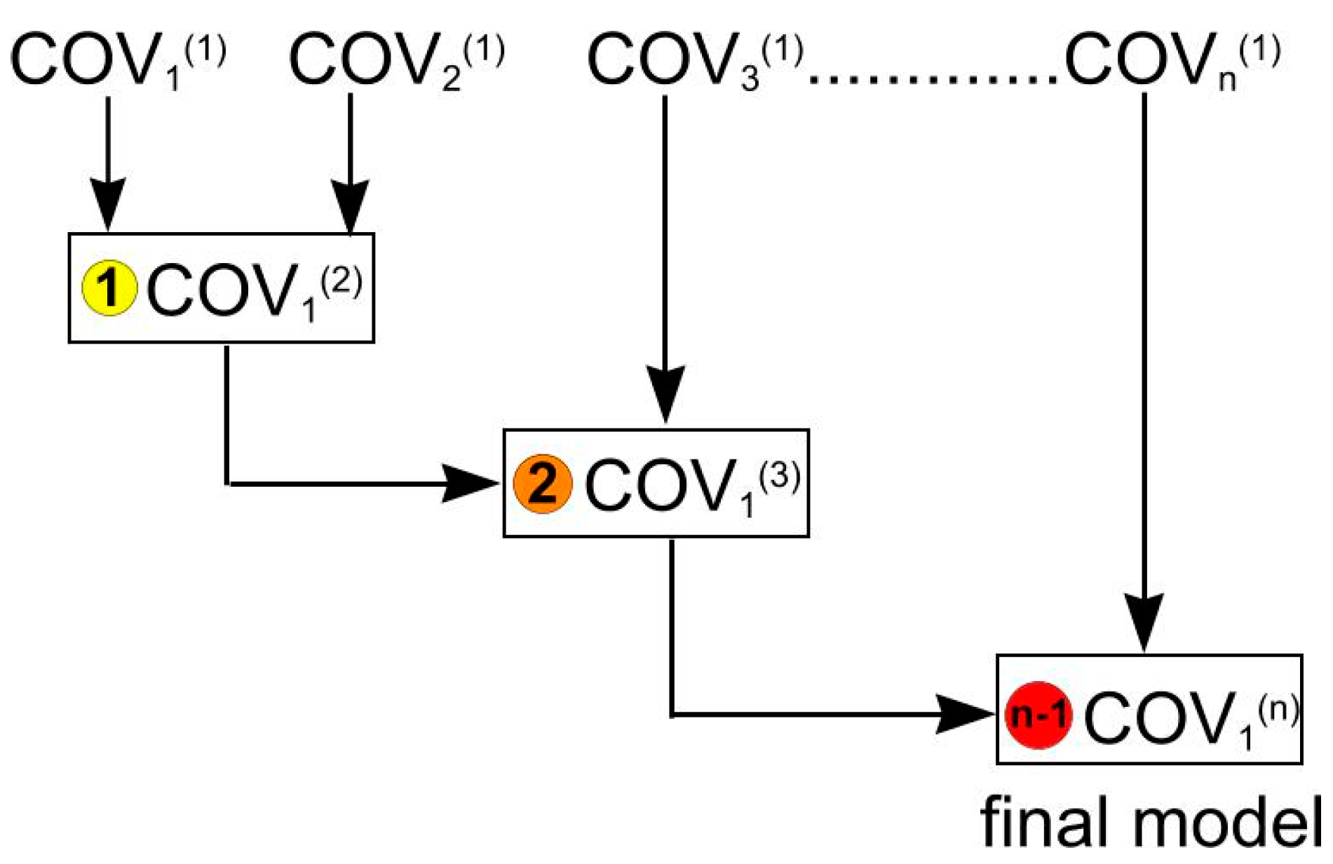
2.2.1. Sequential Hierarchical Modeling

Given the above mentioned properties of the product-sum model, assuming we intend to model COV⁽³⁾ class of the covariance, we could start by separately modeling one COV⁽²⁾ class of the covariance using the product-sum model, and a COV⁽¹⁾ class of the covariance using basic one-dimensional model, and then combining them again using the product-sum model into a final COV⁽³⁾. The approach is depicted in Scheme 1.

This approach, analogous to spatio-temporal modeling in Equation (2), starts by selecting the first pair of independent one-dimensional variograms to be combined into a product-sum model. In the case of separately modeling variability in horizontal and vertical directions and time, it requires first creating the product-sum model for the first arbitrarily selected pair of dimensions; for example, horizontal and vertical directions:

C_h,v(h_h,h_v)⁽²⁾ = a₁C_h(h_h)⁽¹⁾C_v(h_v)⁽¹⁾+a₂C_h(h_h)⁽¹⁾+a₃C_v(h_v)⁽¹⁾

(8)

Second, C_h,v(h_h,h_v)⁽²⁾ and C_t(h_t)⁽¹⁾ are combined into a final product-sum model:

C_h,v,t(h_h,h_v,h_t)⁽³⁾ = a₄C_h,v(h_h,h_v)⁽²⁾C_t(h_t)⁽¹⁾+a₅C_h,v(h_h,h_v)⁽²⁾+a₆C_t(h_t)⁽¹⁾

(9)

After substituting Equation (8) into Equation (9) it yields:

C_h,v,t(h_h,h_v,h_t)⁽³⁾ = a₁a₄C_h(h_h)⁽¹⁾C_v(h_v)⁽¹⁾C_t(h_t)⁽¹⁾ + a₂a₄C_h(h_h)⁽¹⁾C_t(h_t)⁽¹⁾ + a₃a₄C_v(h_v)⁽¹⁾C_t(h_t)⁽¹⁾ +
… + a₁a₅C_h(h_h)⁽¹⁾C_v(h_v)⁽¹⁾ + a₂a₅C_h(h_h)⁽¹⁾ + a₃a₅C_v(h_v)⁽¹⁾ + a₆C_t(h_t)⁽¹⁾

(10)

Two important conclusions follow from Equation (10). First, any n-dimensional variogram (covariance) can be broken down to one-dimensional components following n−1 modeling steps, each comprising the modeling of one product-sum variogram of the lower dimensionality. Second, Equation (10) shows that the order of modeling lower-dimensional variograms is not important, as it converges to the same model. However, the inferred covariance parameters could be slightly different and dependent on the modeling sequence if tolerances are large, though this can be overcome by modeling at-once, as shown in Section 2.2.2. If we start by modeling first the C_h,t(h_h,h_t) in Equation (8), the initial values for a₁–a₆ would be different, yet their products (shown in bold) in Equation (10) would be the same, as they ultimately come from data, which again points to the symmetrical properties of the product sum model with respect to its basic covariance components. The resulting covariance is guaranteed to yield a valid model, as the product of constants a_1·a₄ that multiplies the first term in Equation (10) is always >0, while all other products of constants are ≥0. The four underlined covariance product terms of the final model represent a Hadamard product [38] of two or more positive definite matrices. According to Schur product theorem, a Hadamard product of two positive definite matrices necessarily gives a positive definite matrix [39]. Thus, the resulting model is guaranteed to be valid.

In the original sequential modeling procedure starting from one-dimensional variograms, γ_s,t (h_s,0) and γ_s,t (0, h_t) were modeled by pre-determining a spatial and temporal tolerance within which a pair of data can still be considered collocated or coincident. However, in practice the required tolerance might need to be very large to yield enough data points, which would lead to inaccuracies in the modeling of both one-dimensional and higher-dimensional variograms, given that lower dimensional variograms are building blocks of higher dimensional variogram (see Section 2.2.2 for further discussion).

Furthermore, correctly representing variability along all axes of anisotropy leads to the reduction in the estimated nugget, if nugget-model variograms are used. For example, in a typical spatial-only variography of satellite retrievals, the variography step is preceded by temporal binning, i.e., data from multiple time periods are aggregated and treated as coincident (e.g., [5,6]). The consequence is that ignored variability along the temporal axis ends up being superposed to the spatial variability as its unexplained portion—nugget.

Similarly, the variability within tolerances imposed by the original sequential product-sum modeling procedure [22] gets superposed to the true variability along the actual modeling axis affecting the unexplained portion of variability. By treating not-exactly-collocated and not-exactly-coincident observations as collocated and coincident, modeler allows some of the spatial variability (within tolerance) to affect the separate temporal variogram, and some of the temporal variability to affect the separate spatial variogram, respectively. In this way, separate spatial and temporal variogram models represent an approximation of the separate variogram models that would be obtained using strictly collocated and strictly coincident observations. This issue was not discussed in the original paper by De Iaco et al. [22], although it affects modeling results for the sequential approach (as the nugget has to be modeled in the first step), but not in modeling the “all at once” approach (Section 2.2.2). Thus, we change the approach, and model all parameters at once.

2.2.2. Modeling “All at Once”

To avoid defining a tolerance, we alter the original procedure by estimating all covariance parameters simultaneously. This simultaneous parameter estimation makes the model more applicable to scattered data and data with variable spatial coverage, as is often the case with airborne observations or satellite data. Defining the tolerance followed naturally from the original sequential modeling procedure proposed in De Iaco et al. [22], starting by modeling separate one-dimensional variograms used in subsequent steps to yield a generalized product-sum model. In the original procedure, the first step assumed computing the sample spatial and temporal variograms corresponding to γ_s,t (h_s,0)and γ_s,t (0,h_t):

$${\widehat{\gamma }}_{s,t}\left(r_s,0\right)=\frac{1}{2\left|N\left(r_s\right)\right|}{\displaystyle \sum }_{N\left(r_s\right)}{\left[Z\left(s+h_s,t\right)-Z\left(s,t\right)\right]}^2$$

(11)

$${\widehat{\gamma }}_{s,t}\left(0,r_t\right)=\frac{1}{2\left|M\left(r_t\right)\right|}{\displaystyle \sum }_{M\left(r_t\right)}{\left[Z\left(s,t+h_t\right)-Z\left(s,t\right)\right]}^2$$

(12)

where r_s and r_t were, respectively, the vector lag with spatial tolerance ${\delta }_s$ and the lag with temporal tolerance ${\delta }_t$. |N(r_s)| and |M(r_t)| are the cardinalities of the following sets:

$$N\left(r_s\right)=\{\left(s+h_s,t\right)\in A, \left(s,t\right)\in A: \Vert r_s-h_s\Vert < {\delta }_s\}$$

(13)

$$M\left(r_t\right)=\{\left(s,t+h_t\right)\in A, \left(s,t\right)\in A: \Vert r_t-h_t\Vert < {\delta }_t\}$$

(14)

The need to define the tolerance follows from the fact that, in order to construct separate spatial variogram based on coincident observations (${\widehat{\gamma }}_{s,t}\left(r_s,0\right))$, or separate temporal variogram based on collocated observations (${\widehat{\gamma }}_{s,t}\left(0,r_t\right))$, the observational data set in practice has to be dense, or tolerances have to be relatively large to yield enough data for the construction of variograms. In other words, there are often too few collocated pairs of points that cover a wide range of temporal distances, and coincident points that cover a wide range of spatial distances, which imposes increasing the tolerances. The trade-off is that the variabilities captured by separate variograms become virtually higher, as temporal and spatial variability between pairs of points separated within the tolerance gets superposed on spatial and temporal variability of coincident, and collocated points, respectively. However, if the hyperdimensional variograms are fitted to the raw variograms at once, the need to define tolerances vanish. All variogram parameters are estimated simultaneously, including the ones that correspond to separate spatial and temporal variograms. The fitting procedure exploits all found pairs of points at their exact spatial and temporal distances and fits the optimal parameters at once.

The modeling starts by fitting the V⁽ⁿ⁾ variogram corresponding to Equation (3). into an experimental (or alternatively a raw) variogram, and replacing k using Equation (7). Then the V⁽ⁿ⁻¹⁾ variogram component on the right-hand side of the expression is again substituted using Equation (3) and Equation (7), and maximal dimensionality of the basic variograms is again reduced by one. The procedure is recursively repeated until all variogram terms on the right-hand side have dimensionality one. While the expression itself can be very large, the number of parameters to estimate all at once is relatively small and computationally feasible. For example, to model V⁽³⁾ variogram using common 3-parameter exponential or Gaussian model, it would be required to simultaneously estimate only 9 parameters (nugget, 3 times V⁽¹⁾ sill and range parameters, and two k-parameters). For temporally evolving anisotropic full 3D space, only 12 estimated parameters would be required. Generally, the number of parameters for an n-dimensional variogram to be estimated is 3n.

From a practical standpoint, in the sequential modeling approach, modeling constants k₁–k_n−1 play important roles, since the sill⁽²⁾–sill⁽ⁿ⁾ values are obtained after the k value is optimized in each step. However, in modeling “all at once,” k constants are substituted following Equation (7), and do not appear as important entities over the course of modeling.

3. Application

As an example of how our method can address spatial scaling problems, we explored sensitivity of gross primary productivity (GPP) to spatial variability in photosynthetically-active radiation (PAR). Clouds influence the quantity and quality of light for GPP [40,41]. However, gridded meteorological datasets are often too coarse (~100 km) to resolve mesoscale (~10 km) weather systems (e.g., thunderstorms) that affect PAR. Furthermore, modeled GPP calculated from coarse-resolution PAR can be biased due to nonlinearity in the GPP-PAR relationship. We explored the impact of spatial variability in PAR on GPP, using our kriging method to estimate shortwave radiation from Oklahoma Mesonet stations (PAR was approximated as half the downwelling shortwave radiation; [42]. We modeled GPP as a function of PAR (black curve in Figure 1), using a two-leaf canopy model applied to winter wheat in Oklahoma [43].

The spatio-temporal modeling of PAR was done under a moving window setup [44] in such a way that spatial covariance for every 5-min time slice was modeled separately, allowing sampling of the data within +/−30 preceding and following 5-min time periods. Thus, problems resulting from the non-stationarity of the PAR mean due to the diurnal cycle were avoided. We assumed that the V⁽³⁾ variogram offers an adequate representation of the variability, and treated time, horizontal and vertical distances as orthogonal components in variogram space, and thus modeled separately. The vertical and temporal directions were modeled using Gaussian, and horizontal using an exponential model. After modeling the covariance, we kriged the PAR to a regular ~10 × 10 km grid mimicking the kriging approach in Tadić et al. [6], and obtained the average PAR for May 2006 shown in Figure 1.

We estimated the impact of spatial variability in PAR on GPP, using GPP calculated from spatially-averaged PAR as a basis for comparison. Due to nutrient or other limitations, GPP can become light-saturated, such that further increases in PAR yield diminishing returns for GPP at high PAR values. This saturation effect is characterized by the nonlinear shape of the GPP-PAR curve (Figure 1, black line). Forcing a GPP model with spatially-averaged PAR could lead to overestimated GPP, since the full spatial distribution of PAR would include values in the light-saturated part of the curve while the spatial average would fall closer to the unsaturated part. In that case, higher values of PAR increase average PAR but do not substantially increase average GPP.

Indeed, we found that GPP calculated from the spatially-averaged PAR was up to 1.5 µmol m⁻² s⁻¹ higher (Figure 1, red circle) than the average of GPP calculated from the spatially-variable PAR (Figure 1, blue line). The difference between these two estimates is 24% of the observed standard deviation in daytime half-hourly GPP at a site near Lamont, Oklahoma [43], and indicates the importance of spatial variability in climate drivers of GPP. This likely represents an upper bound on such effects at this site, as the GPP-PAR curve used here has a high degree of nonlinearity to illustrate the utility of our method for a general class of problems. Related problems for which this method is applicable include modeling spatiotemporal variability in soil moisture and leaf area index, and the nonlinear influence of these variables on evapotranspiration and surface energy partitioning [45].

4. Conclusions

This study presents an easy and practical way of modeling spatial variability in cases where hyper-dimensional covariance (variogram) structures are required to describe observed spatial variability. It could be especially useful in modeling anisotropic conditions with multiple axes of anisotropy, often encountered in environmental and ecological sciences, or in cases where multiple units have to be used to span dimensions of interest (e.g., space and time). The method is simpler than classical approaches to modeling anisotropy (see Chiles and Delfiner, [1], for details) and requires fewer parameters to be estimated from the data. It represents an alternative to approaches that use time series and spatial analysis conjointly to represent variability at unsampled locations (e.g., Romanowicz et al. [46]).

We showed that this approach yields admissible hyper-dimensional covariance models using valid lower-dimensional covariance models as basic blocks. It allows a relatively easy modeling of full 3D-anisotropic space evolving in time, a task that so far has been challenging.

We showed that the original sequential product-sum modeling method can yield results slightly different from the method we propose in this study due to the existence of tolerances and a potentially higher estimated nugget. We simplified the modeling approach and made it applicable to sparse data by proposing an “all at once” modeling approach.

One of the deficiencies of this study is the lack of the specific-case analysis of the criteria for choosing a product-sum model and its higher dimensional derivates instead of other covariance models. While it should be the method of choice in modeling the data characterized by negative non-separability, it might not be suitable for data characterized by positive non-separability and pointwise non-separability (both positive and negative). For more information on this topic, please see De Iaco et al. [19], De Iaco and Posa [17] and De Iaco et al. [18].

Many ecological processes are nonlinear and can result in biased predictions when using coarse-resolution datasets to drive ecological models. We presented a straightforward approach to estimate spatiotemporal variability and demonstrated its application to spatial scaling of ecological processes. This approach relaxes previous assumptions regarding isotropicity of variability for hyper-dimensional analysis, which enables applications across a wider range of environmental and ecological problems.

5. Software and/or Data Availability Section

The documented Matlab source code (functions) is available at the ResearchGate website [47]. The code is made available under ‘CC BY’ license terms [48]. The code was developed by Jovan Tadić in Dec 2017 in Matlab 2016a. Contact details: e-mail: [email protected]. It can be run on a personal computer without special requirements. The archive contains Matlab functions used to model 3D covariance structure using three independent variogram models, presented in the article. The size of the zipped archive is 5 kb.

References

1. Chilès, J.-P.; Delfiner, P. Kriging. In Geostatistics: Modeling Spatial Uncertainty, 2nd ed.; John Wiley & Sons, Inc.: Hoboken, NJ, USA, 2012. [Google Scholar] [CrossRef]
2. Stein, M. Statistical methods for regular monitoring data. J. R. Stat. Soc. Ser. B Stat. Methodol. 2005, 67, 667–687. [Google Scholar] [CrossRef]
3. Montero, J.M.; Fernández-Avilés, G.; Mateu, J. Spatial and Spatio-Temporal Geostatistical Modeling and Kriging; Wiley: Chichester, UK, 2015. [Google Scholar]
4. Tadić, J.M.; Ilić, V.; Biraud, S. Examination of geostatistical and machine-learning techniques as interpolators in anisotropic atmospheric environments. Atmos. Environ. 2015, 111, 28–38. [Google Scholar] [CrossRef] [Green Version]
5. Hammerling, D.M.; Michalak, A.M.; O’Dell, C.; Kawa, S.R. Global CO2 distributions over land from the Greenhouse Gases Observing Satellite (GOSAT). Geophys. Res. Lett. 2012, 39, L08804. [Google Scholar] [CrossRef]
6. Tadić, J.M.; Qiu, X.; Yadav, V.; Michalak, A.M. Mapping of satellite Earth observations using moving window block kriging. Geosci. Model Dev. 2015, 8, 1–9. [Google Scholar] [CrossRef]
7. Cressie, N.; Wikle, C. Statistics for Spatio-Temporal Data; Wiley: Hoboken, NJ, USA, 2011; 588p. [Google Scholar]
8. Gneiting, T.; Genton, M.G.; Guttorp, P. Geostatistical space-time models, stationarity, separability and full symmetry. In Statistics of Spatio-Temporal Systems; Finkenstaedt, B., Held, L., Isham, V., Eds.; Monographs in Statistics and Applied Probability; Chapman & Hall/CRC Press: Boca Raton, FL, USA, 2007; pp. 151–175. [Google Scholar]
9. Kyriakidis, P.C.; Journel, A.G. Geostatistical space–time models: A review. Math. Geol. 1999, 31, 651–684. [Google Scholar] [CrossRef]
10. Snepvangers, J.J.J.C.; Heuvelink, G.B.M.; Huisman, J.A. Soil water content interpolation using spatio-temporal kriging with external drift. Geoderma 2003, 112, 253–271. [Google Scholar] [CrossRef]
11. Stein, M. Space–Time Covariance Functions; Technical Rep. 4; Center for Integrating Statistical and Environ Science, University of Chicago: Chicago, IL, USA, 2004. [Google Scholar] [Green Version]
12. Horrell, M.T.; Stein, M.L. Half-spectral space–time covariance models. Spat. Stat. 2017, 19, 90–100. [Google Scholar] [CrossRef]
13. Rodrigues, A.; Diggle, P. A class of convolution-based models for spatio-temporal processes with non-separable covariance structure. Scand. J. Stat. 2010, 37, 553–567. [Google Scholar] [CrossRef]
14. Zastavnyi, V.; Porcu, E. Characterization theorems for the gneiting class of space-time covariances. Bernoulli 2011, 17, 456–465. [Google Scholar] [CrossRef]
15. De Iaco, S.; Myers, D.; Posa, D. On strict positive definiteness of product and product-sum covariance models. J. Stat. Plan. Inference 2011, 141, 1132–1140. [Google Scholar] [CrossRef]
16. De Iaco, S.; Posa, D. Predicting Spatio-Temporal Random Fields: Some Computational Aspects. Comput. Geosci. 2012, 41, 12–24. [Google Scholar] [CrossRef]
17. De Iaco, S.; Posa, D. Positive and Negative Non-Separability for Space-Time Covariance Models. J. Stat. Plan. Inference 2013, 143, 378–391. [Google Scholar] [CrossRef]
18. De Iaco, S.; Posa, D.; Myers, D.E. Characteristics of Some Classes of Space-Time Co-variance Functions. J. Stat. Plan. Inference 2013, 143, 2002–2015. [Google Scholar] [CrossRef]
19. De Iaco, S.; Palma, M.; Posa, D. A General Procedure for Selecting a Class of Fully Symmetric Space-Time Covariance Functions. Environmetrics 2016, 112, 212–224. [Google Scholar] [CrossRef]
20. Heuvelink, G.B.M.; Pebesma, E.; Gräler, B. Space-Time Geostatistics published in Encyclopedia of GIS; Springer International Publishing: Cham, Switzerland, 2017; pp. 1919–1926. [Google Scholar] [CrossRef]
21. De Iaco, S.; Posa, D. Strict positive definiteness in geostatistics. Stoch. Environ. Res. Risk Assess. 2018, 32, 577–590. [Google Scholar] [CrossRef]
22. De Iaco, S.; Myers, D.; Posa, D. Space-time analysis using a general product–sum model. Stat. Probab. Lett. 2001, 52, 21–28. [Google Scholar] [CrossRef]
23. Tadić, J.M.; Michalak, A.M.; Iraci, L.; Ilić, V.; Biraud, S.C.; Feldman, D.R.; Built, T.; Johnson, M.S.; Loewenstein, M.; Jeong, S.; et al. Elliptic Cylinder Airborne Sampling and Geostatistical Mass Balance Approach for Quantifying Local Greenhouse Gas Emissions. Environ. Sci. Technol. 2017, 51, 10012–10021. [Google Scholar] [CrossRef]
24. Brock, F.V.; Crawford, K.C.; Elliott, R.L.; Cuperus, G.W.; Stadler, S.J.; Johnson, H.W.; Eilts, M.D. The Oklahoma Mesonet—A technical overview. J. Atmos. Ocean. Technol. 1995, 12, 5–19. [Google Scholar] [CrossRef]
25. McPherson, R.A.; Fiebrich, C.A.; Crawford, K.C.; Kilby, J.R.; Grimsley, D.L.; Martinez, J.E.; Basara, J.B.; Illston, B.G.; Morris, D.A.; Kloesel, K.A.; et al. Statewide monitoring of the mesoscale environment: A technical update on the Oklahoma Mesonet. J. Atmos. Oceanic Technol. 2007, 24, 301–321. [Google Scholar] [CrossRef]
26. Tadić, J.M.; Qiu, X.; Miller, S.; Michalak, A.M. Spatio-temporal approach to moving window block kriging of satellite data V1.0. Geosci. Model Dev. 2017, 10, 709–720. [Google Scholar] [CrossRef]
27. Christakos, G. On the problem of permissible covariance and variogram models. Water Resour. Res. 1984, 20, 251–265; [Google Scholar] [CrossRef]
28. Dimitrakopoulos, R.; Luo, X. Spatiotemporal modeling: Covariances and ordinary kriging systems. In Quantitative Geology and Geostatistics, Geostatistics for the Next Century; Dimitrakopoulos, R., Ed.; Springer: Dordrecht, The Netherlands, 1994; pp. 88–93. [Google Scholar]
29. Rouhani, S.; Hall, T.J. Space-Time Kriging of Groundwater Data. In Geostatistics; Armstrong, M., Ed.; Kluwer Academic Publishers: Dordrecht, The Netherlands, 1989; Volume 2, pp. 639–651. [Google Scholar]
30. De Cesare, L.; Myers, D.E.; Posa, D. Spatio-temporal modelling of SO2 in Milan district. In Geostatistics Wollongong; Baafi, E.Y., Schofield, N.A., Eds.; Kluwer Academic Publishing: Dordrecht, The Netherlands, 1996; pp. 1031–1042. [Google Scholar]
31. Cressie, N.; Huang, H.C. Classes of nonseperable, spatio-temporal stationary covariance functions. J. Am. Stat. Assoc. 1999, 94, 1–53. [Google Scholar] [CrossRef]
32. Guo, L.; Lei, L.; Zeng, Z. Spatiotemporal correlation analysis of satellite-observed CO2: Case studies in China and USA. In Proceedings of the IEEE International Geoscience and Remote Sensing Symposium (IGARSS), Melbourne, Australia, 21–26 July 2013. [Google Scholar]
33. Zeng, Z.; Lei, L.; Guo, L.; Zhang, L.; Zhang, B. Incorporating temporal variability to improve geostatistical analysis of satellite-observed CO2 in China. Chin. Sci. Bull. 2013, 58, 1948–1954. [Google Scholar] [CrossRef]
34. Zeng, Z.-C.; Lei, L.; Strong, K.; Jones, D.B.A.; Guo, L.; Liu, M.; Deng, F.; Deutscher, N.M.; Dubey, M.K.; Griffith, D.W.T.; et al. Global land mapping of satellite-observed CO2 total columns using spatio-temporal geostatistics. Int. J. Digit. Earth 2017, 10, 426–456. [Google Scholar] [CrossRef] [Green Version]
35. De Cesare, L.; Myers, D.; Posa, D. Estimating and modeling space–time correlation structures. Stat. Prob. Lett. 2001, 51, 9–14. [Google Scholar] [CrossRef]
36. De Cesare, L.; Myers, D.E.; Posa, D. Product–sum covariance for space–time modeling: An environmental application. Environmetrics 2001, 12, 11–23. [Google Scholar] [CrossRef]
37. Salmon, M.M. Introduction to Logic and Critical Thinking, 6th ed.; Cengage Learning: Boston, MA, USA, 2012. [Google Scholar]
38. Million, E. The Hadamard Product. 2007. Available online: http://buzzard.ups.edu/courses/2007spring/projects/million-paper.pdf (accessed on 9 January 2019).
39. Mathias, R. Matrix completions, norms and Hadamard products. Proc. Am. Math. Soc. 1993, 117, 905–918. [Google Scholar]
40. Baldocchi, D. FLUXNET: A new tool to study the temporal and spatial variability of ecosystem-scale carbon dioxide, water vapor, and energy flux densities. Bull. Am. Meteorol. Soc. 2001, 82, 2415–2434. [Google Scholar] [CrossRef] [Green Version]
41. Vilà-Guerau de Arellano, J.; Ouwersloot, H.G.; Baldocchi, D.; Jacobs, C.M.J. Shallow cumulus rooted in photosynthesis. Geophys. Res. Lett. 2014, 41, 1796–1802. [Google Scholar] [CrossRef]
42. Lambers, H.; Stuart Chapin, F.S.; Pons, T.L. Photosynthesis. In Plant Physiological Ecology; Springer: New York, NY, USA, 2008; pp. 11–99. [Google Scholar]
43. Williams, I.N.; Riley, W.J.; Kueppers, L.M.; Biraud, S.C.; Torn, M.S. Separating the effects of phenology and diffuse radiation on gross primary productivity in winter wheat. J. Geophys. Res. Biogeosci. 2016, 121, 1903–1915. [Google Scholar] [CrossRef]
44. Haas, T.C. Lognormal and moving window methods of estimating acid deposition. J. Am. Stat. Assoc. 1990, 85, 950–963. [Google Scholar] [CrossRef]
45. Bagley, J.E.; Kueppers, L.M.; Billesbach, D.P.; Williams, I.N.; Biraud, S.C.; Torn, M.S. The influence of land cover on surface energy partitioning and evaporative fraction regimes in the U.S. Southern Great Plains. J. Geophys. Res. Atmos. 2017, 122, 5793–5807. [Google Scholar] [CrossRef]
46. Romanowicz, R.; Young, P.; Brown, P.; Diggle, P. A recursive estimation approach to the spatio-temporal analysis and modelling of air quality data. Environ. Model. Softw. 2006, 21, 759–769. [Google Scholar] [CrossRef]
47. Tadić, J. Hyperdimensional Variography Code. Available online: https://www.researchgate.net/publication/313387764_Hyperdimensional_Variography_Code (accessed on 10 January 2019).
48. Creative Commons. Available online: https://creativecommons.org/licenses/ (accessed on 10 January 2019).
Scheme 1. The sequence of necessary steps (1…(n−1)), to model COV(n) class of covariance using the product-sum model sequentially, starting from one-dimensional basic covariance (variogram) models COV1(1)-COVn(1).
Atmosphere 10 00148 sch001
Figure 1. Application of kriged shortwave radiation (i.e., PAR) to estimate gross primary productivity (GPP) over a 2.5° longitude × 2.5° latitude region (~220 km) in central Oklahoma. The black curve illustrates the nonlinear relationship between GPP and PAR from a canopy model. The histogram shows the distribution of PAR values within the region on May 30 of 2006 (16:00–6:30 local time). Due to the saturation of GPP at high PAR, estimates of GPP from the spatially-averaged PAR (red circle) are higher than the actual regional-scale GPP (blue line).
Atmosphere 10 00148 g001