Article

Analysis of Two Dimensionality Reduction Techniques for Fast Simulation of the Spectral Radiances in the Hartley-Huggins Band

Remote Sensing Technology Institute, German Aerospace Center (DLR), 82234 Oberpfaffenhofen, Germany
*
Author to whom correspondence should be addressed.
Atmosphere 2019, 10(3), 142; https://doi.org/10.3390/atmos10030142
Submission received: 22 February 2019 / Revised: 12 March 2019 / Accepted: 13 March 2019 / Published: 16 March 2019
(This article belongs to the Special Issue Radiative Transfer Models of Atmospheric and Cloud Properties)

Abstract

:
The new generation of atmospheric composition sensors such as TROPOMI is capable of providing spectra of high spatial and spectral resolution. To process this vast amount of spectral information, fast radiative transfer models (RTMs) are required. In this regard, we analyzed the efficiency of two acceleration techniques based on the principal component analysis (PCA) for simulating the Hartley-Huggins band spectra. In the first one, the PCA is used to map the data set of optical properties of the atmosphere to a lower-dimensional subspace, in which the correction function for an approximate but fast RTM is derived. The second technique is based on the dimensionality reduction of the data set of spectral radiances. Once the empirical orthogonal functions are found, the whole spectrum can be reconstructed by performing radiative transfer computations only for a specific subset of spectral points. We considered a clear-sky atmosphere where the optical properties are defined by Rayleigh scattering and trace gas absorption. Clouds can be integrated into the model as Lambertian reflectors. High computational performance is achieved by combining both techniques without losing accuracy. We found that for the Hartley-Huggins band, the combined use of these techniques yields an accuracy better than 0.05% while the speedup factor is about 20. This innovative combination of both PCA-based techniques can be applied in future works as an efficient approach for simulating the spectral radiances in other spectral regions.

1. Introduction

The new generation of atmospheric composition sensors such as the TROPospheric Ozone Monitoring Instrument (TROPOMI) delivers a great amount of data. Extracting the information about geophysical parameters (e.g., trace gas concentrations) from spectral radiances requires high-performance computing. The key component of retrieval algorithms is the radiative transfer models (RTMs), which convert optical parameters of the atmosphere (i.e., input space) into spectral radiances (i.e., output space). In hyper-spectral remote sensing retrieval applications, the radiative transfer computations are the bottleneck in the whole processing chain. In this regard, acceleration techniques for hyper-spectral RTMs have to be developed [1]. The correlated k-distribution [2], the exponential-sum fitting transmittance [3], the radiance sampling method [4], and the optimal spectral mapping method [5] are examples of them. Essentially, these techniques do not compute spectral radiances in a line-by-line manner, but rather they take into account the interdependency between spectral channels or group them accordingly, thereby reducing the total number of calls to RTMs.
In the RTM development, there has been a rapid rise in the use of the data reduction concept, e.g., the principal component analysis (PCA). The acceleration techniques based on PCA can be broadly categorized into two groups: data reduction of optical parameters (input space reduction) and data reduction of spectral radiances (output space reduction).
The input space reduction technique was proposed by Natraj et al. [6], and its main idea is to reproduce the residual between the accurate and the approximate RTMs in the reduced space of optical parameters. This approach has the following attributes:
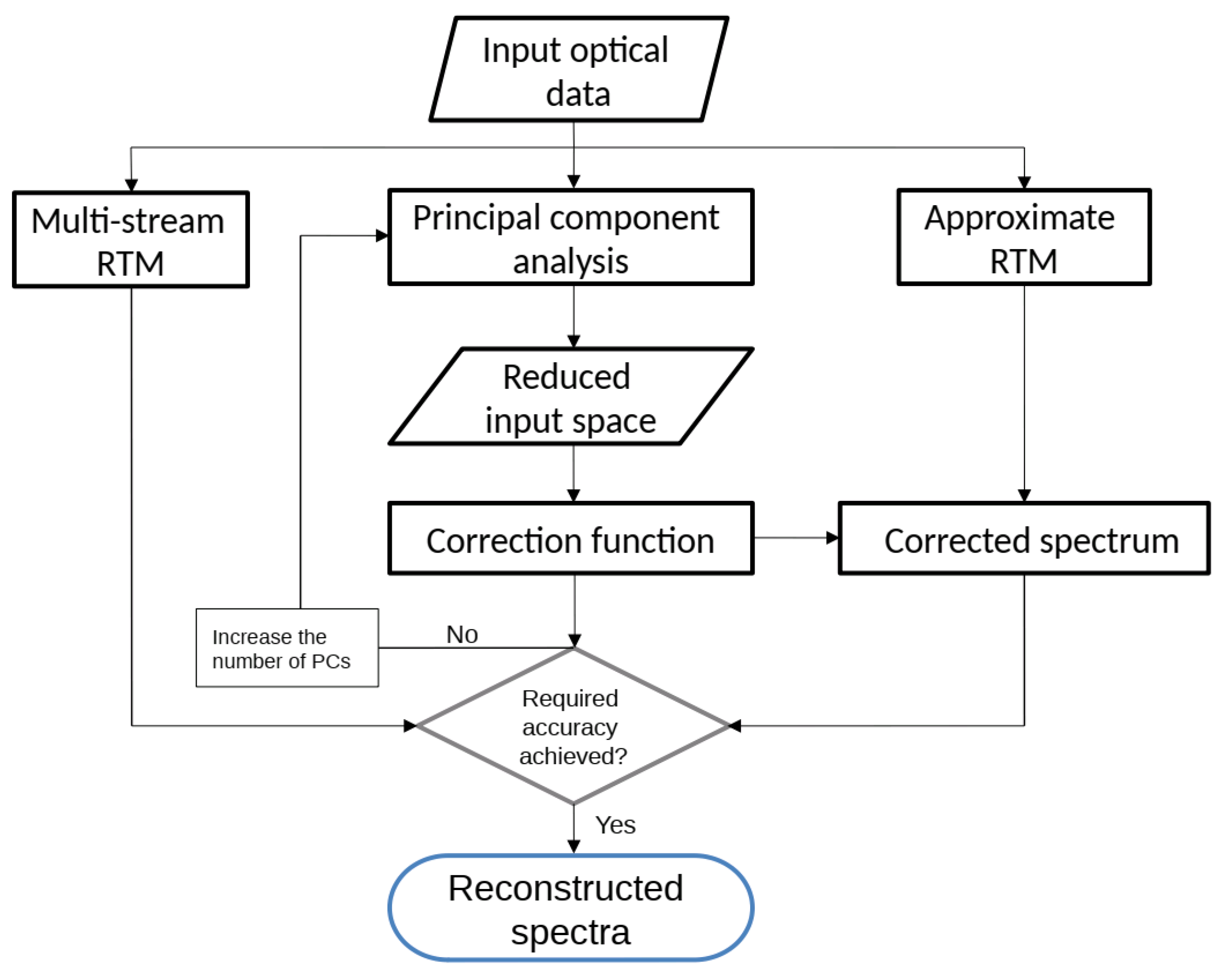
  • the approximate model is a two-stream radiative transfer model, while the accurate model is a multi-stream radiative transfer model;
  • the PCA is used to reduce the dimensionality of the optical parameters of the atmospheric system;
  • the dependency of the correction factor on the optical parameters is modeled by a second-order Taylor expansion about the mean value of the optical parameters.
Previously, this approach was applied for simulating the spectra in the O2 A-band [6], the Huggins band [7], and the CO2 bands [8,9]. Kopparla et al. [10] applied a similar approach to modeling the radiances in the wide spectral range (0.3–3000 nm). In all cases, authors reported that the root-mean-square errors of the computed radiances are about 0.3%, yet achieving almost a 10-fold increase in speed.
In the output space reduction technique, the principal component analysis (PCA) is used to map the spectral radiances into a lower-dimensional subspace and to obtain a set of empirical orthogonal functions. The spectrum at full spectral resolution can be reproduced by computing the radiances only at certain wavelengths. Such an approach is used in several fast RTMs (e.g., PCRTM [11], RTTOV [12] and others [13,14]) and retrieval algorithms [15,16]. To select the most representative spectral subsets, the spectral sampling methods are used (see, e.g., [11,14] and references therein).
Note that, although both techniques are often called the same (namely “PCA-based RTMs”), they are fundamentally different. In the first case, PCA is applied to a data set of optical parameters, comprising the total optical thicknesses and the single scattering albedos for all given atmospheric layers and wavelengths. In the second case, PCA is applied to the data set of spectral radiances.
In the current study, we investigate the efficiency of the dimensionality reduction technique of optical parameters in the Hartley-Huggins band and improve upon the methods to maximize the advantages of the data reduction concept. First, we examine the efficiency of the input space reduction technique for simulating TROPOMI signals in the ultraviolet spectral range, which is typically used for ozone retrieval [17]. As approximate models, we consider the two-stream model and the single-scattering model. The spectral splitting is applied to improve the accuracy of the method. Second, we analyze the effect of including higher-order terms in the Taylor expansion of the correction function. Third, we apply the output space reduction technique to the data set of synthetic TROPOMI spectra and analyze the possible benefits of it. Fourth, we show how the input space reduction technique can be used in conjunction with the output space reduction method. The paper is organized as follows. In Section 2 we explain the input space reduction technique. The output space reduction and the spectral sampling techniques are described in Section 3. In Section 4, we evaluate the performance of these methods and discuss the combined usage of them.

2. Input Space Reduction Technique

2.1. Radiative Transfer Models

Many existing RTMs are based on the discrete ordinate method [18]. The number of streams (discrete ordinates) in the polar hemisphere, N do , is an important parameter controlling the computational time and accuracy. Thus, RTMs are called “multi-stream” if N do 2 and “two-stream” (TS) if N do = 1 . The simplest analytical RTM is the single-scattering (SS) model, in which multiple scattering events are neglected. The TS and the SS RTMs are considerably faster than the multi-stream models [7]. However, they suffer from a lack of accuracy. TS and SS models are taken in this study as approximate models for fast computations of the spectral radiances. Then the multi-stream model is applied to correct them.
In this study, the multi-stream model is based on the discrete ordinate method with matrix exponential (DOME) [19,20,21] with 16 streams per hemisphere. Regarding the two-stream model, two comments are in order:
  • the radiation field is found as a sum of the single-scattering solution and the multiple scattering term;
  • in the multiple scattering computations the delta-M truncation method [3] is applied, while for the single-scattering term the exact phase function is used [22].

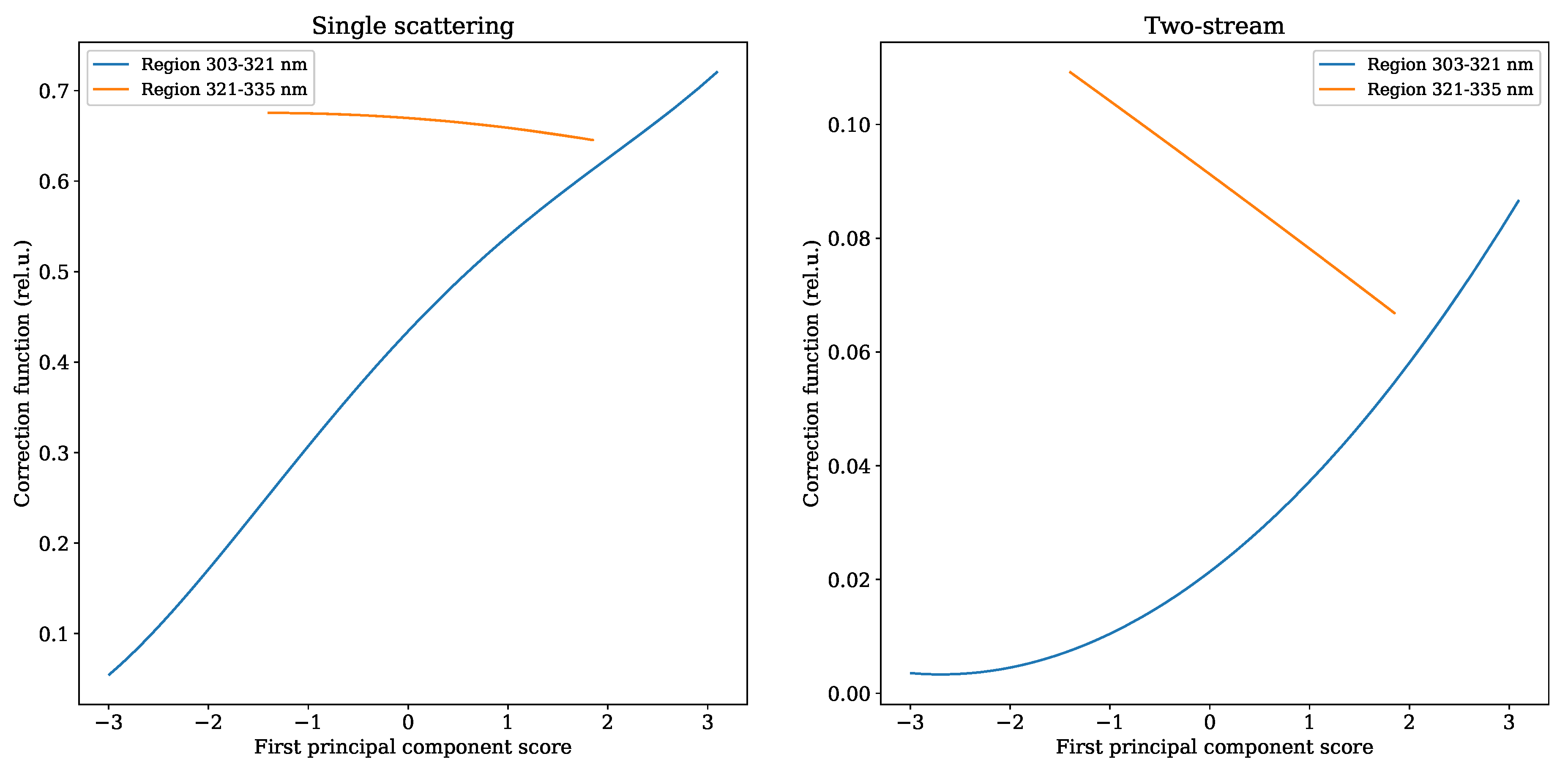
2.2. Correction Function in the Reduced Input Space

Considering a discretization of the atmosphere in L layers, we define an N-dimensional vector x w , for each wavelength λ w w = 1 , , W , by
x w T = ln τ 1 λ w , , ln τ L λ w , ln ω 1 λ w , , ln ω L λ w ,
where τ k and ω k are the optical thickness and the single-scattering albedo of the k-th layer, respectively, and N = 2 L . Thus, the vector x w encapsulates the wavelength variability of the optical parameters, which are the input parameters of the radiative transfer code. By using PCA, we find an M-dimensional subspace spanned by a set of linear independent vectors (empirical orthogonal functions) q k k = 1 M such that the centered (mean-removed) data x w - x ¯ lie mainly on this subspace, i.e.,
x w x ¯ + k = 1 M y w k q k , w = 1 , , W ,
where y w k are the principal component (PC) scores.
Let us define a correction function f x w as follows:
f x w = ln L x w L A x w ,
where L A x w is the radiance provided by the approximate model (here A stands for “approximate” and refers to SS and TS models), and L x w is the radiance simulated by the multi-stream model. Introducing Δ x w = k = 1 M y w k q k , we consider the Taylor expansion of f x w around x ¯ in the direction Δ x w up to fourth order. For computational simplicity, we neglect the mixed directional derivatives and use central differences to approximate the directional derivatives. Since M < N (and in practice M N ), it leads to a substantial reduction of the computational time. The final result for the correction function reads as
f x w f x ¯ + 1 2 k = 1 M f k + - f k - y w k + 1 2 k = 1 M f k + - 2 f x ¯ + f k - y w k 2 + + 1 12 k = 1 M f k + 2 - 2 f k + + 2 f k - - f k - 2 y w k 3 + + 1 24 k = 1 M f k + 2 - 4 f k + + 6 f x ¯ - 4 f k - + 2 f k - 2 y w k 4 ,
where f k ± n = f x ¯ ± n q k , being h either k or k + 1 . Once the correction function is computed, the results of the approximate RTM can be converted into those of the multi-stream RTM by using (3). A schematic representation of the input data processing is shown in Figure 1.
To improve the accuracy of the input space reduction technique, PCA can be combined with the clustering of the data space, involving a two-step procedure [23]: (1) clustering of the input data space into disjoint regions (groups of wavelengths), and (2) dimensionality reduction within each region by using PCA. Thus, each region (group of wavelengths) is characterized by its own orthogonal basis, and so, by its own set of correction factors. If P is the number of disjoint regions, then ( 2 M + 1 ) P calls of the multi- and two-stream models are required to compute the correction function.

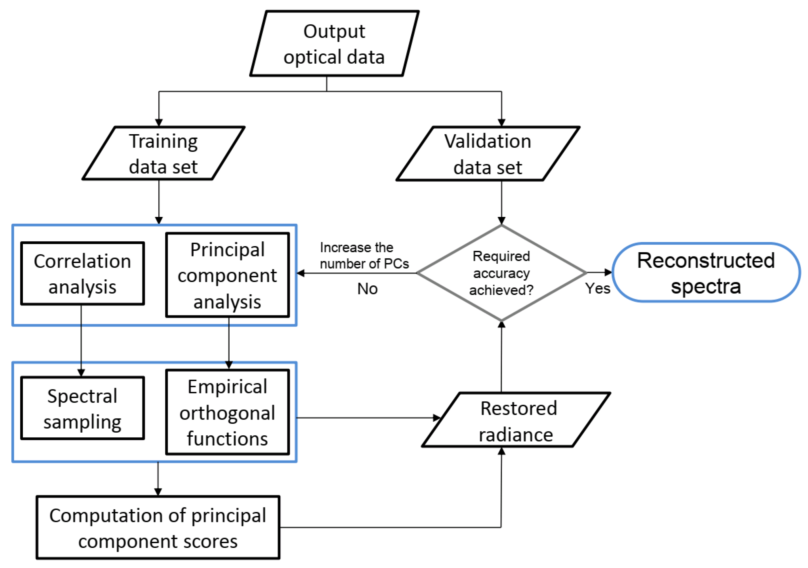
3. Output Space Reduction Technique

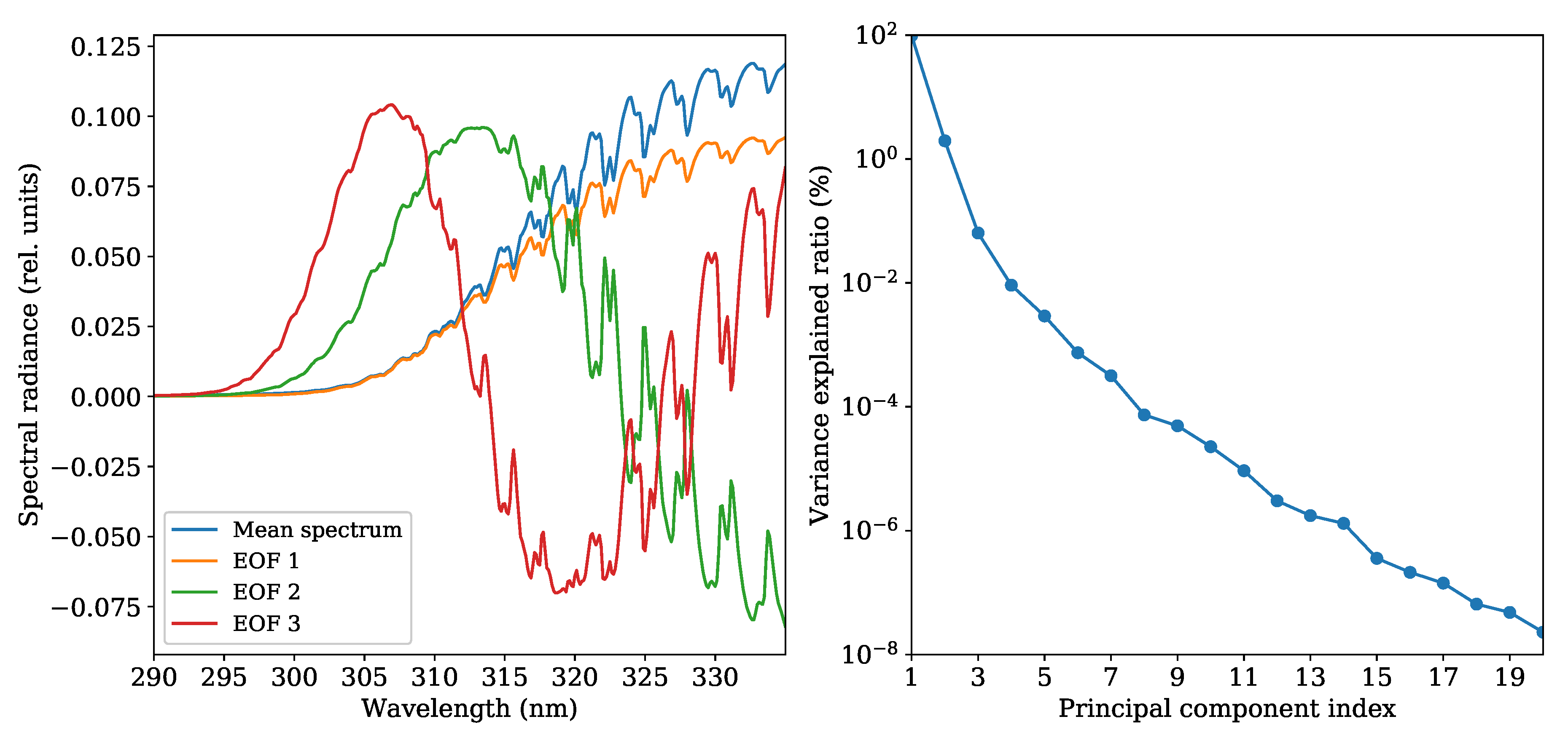
3.1. PCA Description

Let y = y λ 1 , y λ 2 , , y λ W be a row-vector of radiances at W wavelengths λ w w = 1 , , W . A set of S spectra is assembled into a matrix Y whose i-th row is y i . Then, a spectrum y i can be represented in a new basis system as follows:
y i = y ¯ + j = 1 W t i j f j .
Here, y ¯ = i = 1 S y i / S is the sample mean of the spectra (the average spectrum), t i j is the j-th coordinate of the vector y i in the new basis system and f j = f j λ 1 , f j λ 2 , , f j λ W is the j-th basis vector. Next, the spectrum y i is projected onto the J-dimensional subspace ( J < W ) as follows:
y i y ¯ + j = 1 J t i j f j ,
or in matrix form:
Y Y ¯ + T F ,
where Y ¯ = y ¯ , , y ¯ , F = f 1 , f 2 , , f J T and T is the matrix whose entries are t i j i = 1 , , S j = 1 , , J . The superscript T stands for “transpose”. The transformation (6) can be done by using PCA [24]. Then the basic vectors f j in (6) are referred to as “principal components” (PCs) or empirical orthogonal functions (EOFs), while the coordinates t i j in the new coordinate system and the corresponding matrix T are called “principal component scores”. Considering a spectral decomposition of the covariance matrix cov Y , Y C Y :
C Y = E Λ E T ,
where E is the eigenvector matrix and Λ is the diagonal matrix of eigenvalues, the EOFs are taken as J eigenvectors related to the J most significant eigenvalues. The PC scores are then computed as follows:
T = Y - Y ¯ F T .

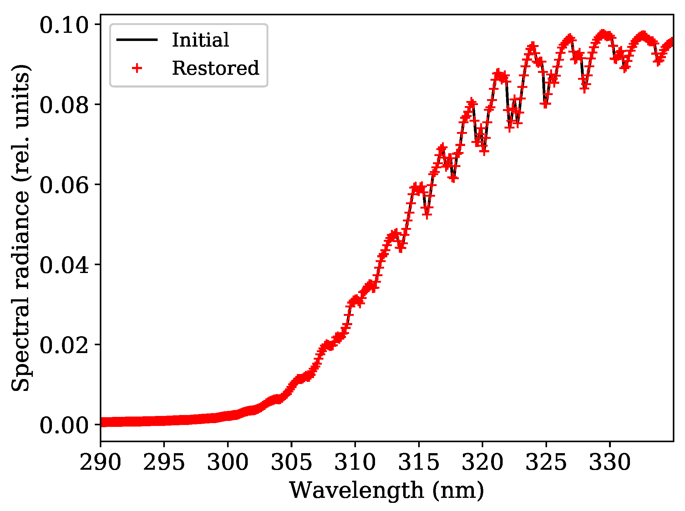
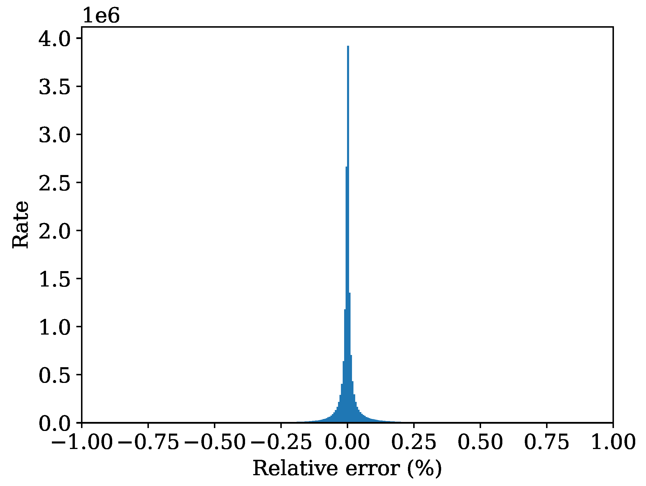
3.2. Reconstruction of the Full Resolution Spectrum

Let us consider a method of reconstruction of the full resolution spectrum containing W spectral points using J monochromatic radiances, given J < W . Assume that we have precomputed a data set of spectra. By applying PCA to it, EOFs are obtained. The theory of PCA discussed in Section 3.1, reveals a linear relationship between PC scores and monochromatic radiances:
y λ y ¯ λ + t 1 f 1 λ + + t J f J λ .
This approach requires a set of precomputed EOFs which is derived from a training data set of simulated spectra. Hence, for a given set of J EOFs and J spectral points, it is possible to obtain a closed linear system of J equations:
y λ 1 = y ¯ λ + t 1 f 1 λ 1 + + t J f J λ 1 , y λ 2 = y ¯ λ + t 1 f 1 λ 2 + + t J f J λ 2 , y λ J = y ¯ λ + t 1 f 1 λ J + + t J f J λ J .
The key point here is that the radiance values in J spectral points { λ j } j = 1 , , J are represented through the same EOFs. Then, by solving (11) we obtain the PC scores, and by using (6) the full spectrum at W spectral points can be readily restored.
The number of principal components J can either be tuned empirically or chosen by using semi-empirical rules (see e.g., [25]). Essentially, the number J depends on the desired level of variance to be captured by the principal components.

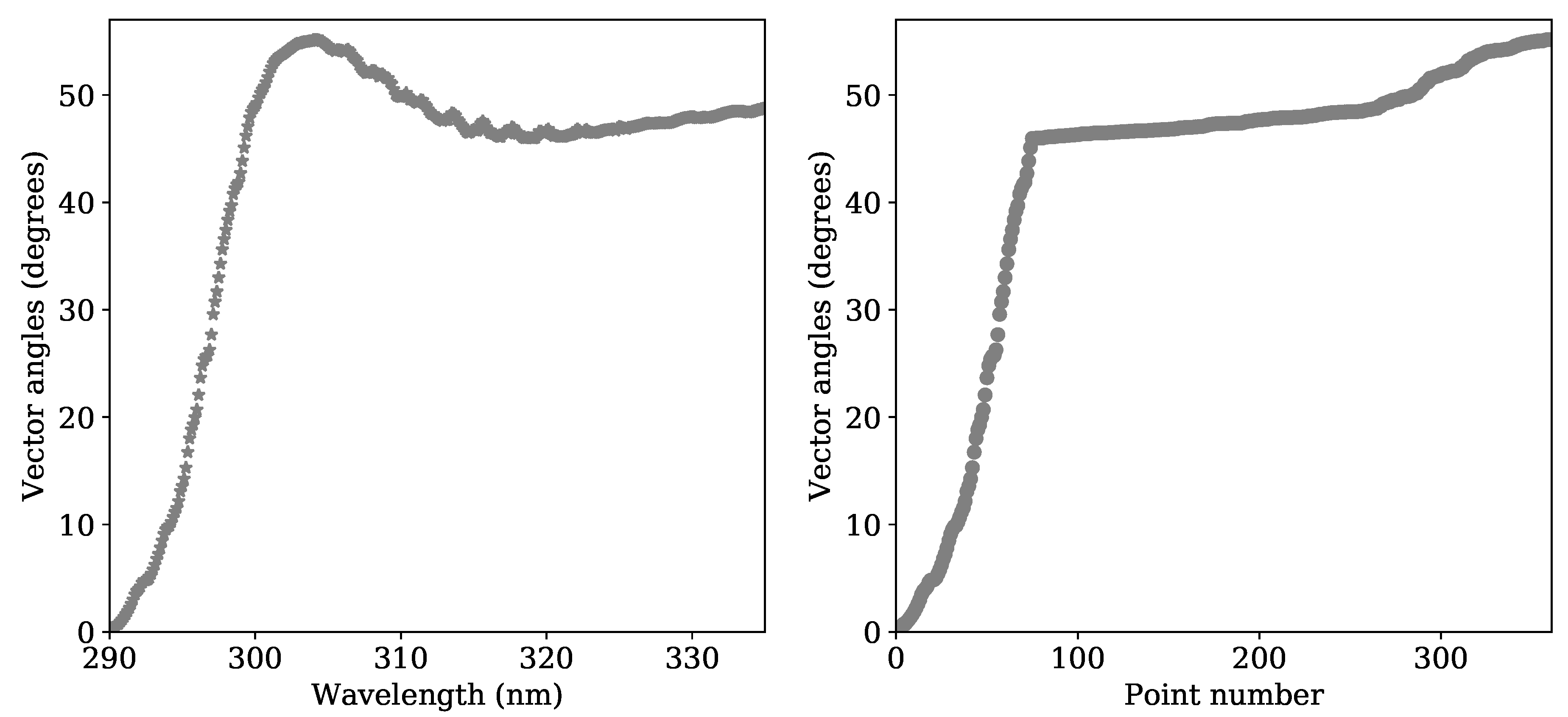
3.3. Spectral Sampling

Regarding the choice of wavelengths, in [11] a method is proposed for selecting the location of monochromatic wavelengths by using a correlation function. This method involves the following steps:
  • the correlation coefficients are computed for the radiance values and then converted to vector angles by an arccosine function;
  • the spectral data are rearranged according to the magnitudes of the correlation coefficients;
  • the monochromatic radiances are selected with equal distances in the space of correlation coefficients.
In [14], alternative techniques such as the equal sampling method and the optimization technique are considered.
To summarize, the output space reduction technique can be used in the following way. For the input data set containing optical parameters of the atmosphere for a set of wavelengths, the monochromatic radiative transfer solver is called for each wavelength. That produces a data set of spectra which is divided into a training data set and a validation data set. By applying PCA and the correlation analysis to the training set, the system of EOFs is computed and an appropriate subset of spectral points is chosen (that is the spectral sampling procedure). These two outputs are stored and used later for computing the PC scores for the validation data set. The spectra at the full spectral resolution are restored using (10) and the error of this reconstruction is estimated. If the error is larger than required, then the number of preserved principal components J is increased. The schematic representation of the output space reduction technique is shown in Figure 2.

4. Results

4.1. Dimensionality Reduction of the Optical Parameters in the Hartley-Huggins Band

In this section, we simulate the backscatter signal of the TROPOMI instrument. The spectra are computed with a spectral resolution of 0.125 nm in the spectral interval between 290 and 335 nm, incorporating the longer part of the Hartley band (200–310 nm) and the shorter part of the Huggins band (320–360 nm). Thus, each spectrum contains 361 spectral points.
The simulations are performed for a clear sky model atmosphere and a Lambertian surface albedo of 0.1. The total optical property inputs are given by Rayleigh scattering [26] by atmospheric molecules and trace gas absorption. Additional cloud properties are neglected in the simulated spectra. To represent cloudy scenes, the effective scene approximation [27] can be used, assuming clouds as Lambertian reflectors. In this case, the cloud top is treated as a reflecting surface characterized by internal surface closure [28]. The Brion–Daumont–Malicet cross sections are used for ozone. Regarding other trace gas species in the spectral range of interest, SO2 and NO2 absorptions are very weak compared to that of ozone, and thus both species are not included in the model. The atmosphere is discretized into 14 layers. The top of the atmosphere is at 50 km. The solar zenith angle, viewing zenith angle and relative azimuth angle are 45 , 35 and 90 , respectively. The simulations are performed on a personal computer with 16 GB RAM and processor Intel(R) Core(TM) i7-6700 CPU @ 3.40 GHz.
Firstly, we compute the radiances of the three RTMs. Figure 3a shows the simulated spectra computed with the multi-stream, TS and SS models. As expected, the TS and SS radiances are inaccurate with maximum errors of about 10% and 30%, respectively. Since the predicted radiances of TS and SS models are inaccurate, three steps are followed in order to improve the accuracy and the computational time: (1) the full spectrum is divided into disjoint regions to apply PCA to each region; (2) a correction function is computed for the different number of PCs and spectral regions; (3) the Taylor expansion up to fourth-order is computed for each spectral region.
Thus, following step (1), we distinguish between three cases depending on the division of the spectral regions:
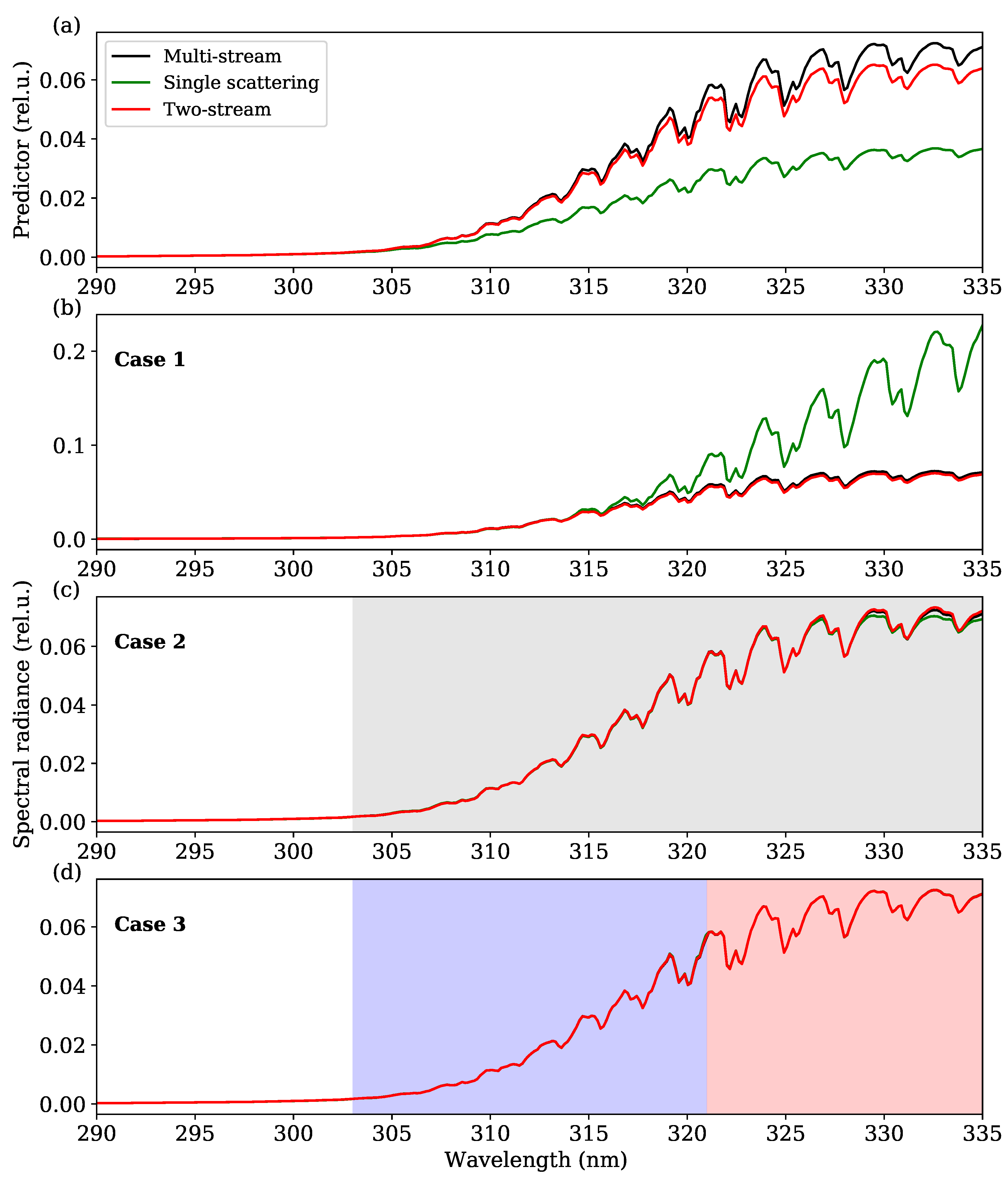
  • Case 1: considering the whole spectral range of 290–335 nm.
  • Case 2: considering two intervals of 290–303 nm and 303–335 nm.
  • Case 3: considering three intervals: 290–303 nm, 303–321 nm and 321–335 nm.
Figure 3b illustrates the spectra when this method is applied to the whole spectral range of 290–335 nm (Case 1). Although the accuracy of the TS model is significantly improved, the mean relative errors are still high (reaching 52% and 2.8% for the SS and TS models, respectively). Note that, due to the high variability in the optical properties over the whole spectral range, the use of input space reduction leads to worse results for the SS model as compared to the TS model.
To reduce the variability of the optical parameters, we compute the spectral range 290–303 nm just by using the single-scattering model (without applying PCA) since the mean error was below 1%. The remaining spectral interval 303–335 nm is computed as before (Case 2). The results are shown in Figure 3c. The gray region corresponds to the domain in which the dimensionality reduction of optical parameters is applied. In this case, the errors are below 3% for the SS model and 0.8% for the TS model.
Finally, in Case 3, three sub-intervals are considered. The single-scattering model was applied to the spectral range 290–303 nm as in Case 2. The input space reduction technique was applied to the remaining two sub-intervals: 303–321 nm and 321–335 nm. Figure 3d shows good agreement between the multi-stream model and the corrected SS/TS models. Note that the accuracy and the computational time strongly depend on the number of preserved principal components (M) and the order of the Taylor expansion, as indicated in Table 1 for Case 3. Here the main conclusion is that the error decreases when M and the expansion order of the Taylor series increase and vice versa.
In all the considered cases, the TS model is more accurate than the SS model. This result is expected since the TS model includes the SS model and estimates the multiple scattering term (approximately, though). The accuracy of the SS and TS models is significantly improved by the correction procedure in (3). This means that the information about the multi-stream solution is contained in the optical data and can be retrieved by using machine learning algorithms, and the input space reduction technique can be considered as representative of them. Here we are confronted with the ad hoc learning, i.e., the algorithm extracts the most informative part of the data and predicts the correct solution using the computations in the reduced data space.
The explained variances of the first PC score in the spectral region 303–321 nm and 321–335 nm are 98.32% and 99.76% respectively, while those for the second PC score in the same regions are 1.63% and 0.21%, respectively. The correction functions are highly correlated with the first PC score and depend smoothly on the first PC score, as shown in Figure 4. However, as it follows from Table 1, the use of just one PC score leads to a loss in accuracy. Therefore, the correction function is highly sensitive to the high order PC scores and the classical methods of estimating the appropriate number of PC scores may fail.
The computational times are listed in Table 2 for Case 3 since it provides the most accurate spectral radiances among the three cases. Two conclusions follow from the table:
  • the increase in the number of PC scores results in the increase of the computational time. However, this increase is not significant (0.05 s per PC score, i.e., ≈1% from the total computational time). Therefore, it is recommended to choose M 3 .
  • the TS model is 40 times slower than the SS model for simulating the approximate spectra. However, the overall computational times differ by a factor of 2. Given that the TS model is more accurate than the SS model (as it has been shown in Table 1), it is recommended to use the TS model.
Note that the computational time for the multi-stream model called for each spectral point is ∼6.8 s. Thus, the input space reduction technique provides the performance enhancement of about 10 times depending on the model used, the number of PC scores, M, and the expansion order of the Taylor series.

4.2. Principal Component Analysis of the Data Set of Spectral Radiances

In this section, we examine the efficiency of the output space reduction technique. For that purpose, we generate a data set consisting of 2 × 10 5 spectra. The following parameters are varied for the generation of radiance spectra: the solar zenith angle, the viewing zenith angle, the relative azimuth angle, the surface albedo, the ozone total column, the surface height, and the temperature. The smart sampling technique [29] based on Halton sequences [30] is employed to optimally cover the multi-dimensional input space and to concurrently minimize the number of samples generated to represent the output space.
The data set of spectra is divided into a training data set and a validation data set (see Figure 2). By applying PCA to the training data set, the system of EOFs is computed (see Figure 5 left). The right plot in Figure 5 shows that almost 99.9% of the variance in the output data can be explained just with J = 2 principal components.
Figure 6 illustrates the spectral sampling procedure [11]. The left panel in Figure 6 shows an example of the arccosine function of the correlation coefficients as a function of the wavelength, while the right panel in Figure 6 shows the resulting plot with rearranging the arccosine function of the correlation coefficients. By using this technique, J = 30 wavelengths are identified.
Next, the EOFs and J wavelengths are saved in the memory and reused for computing PC scores for the validation data set. The spectra at a full resolution are restored using Equation (10). Figure 7 shows one example of the restored spectrum in the Hartley-Huggins band. The histogram of the relative error of the restored spectra from the validation data set is shown in Figure 8. The mean relative error of the spectra is 0.00023% with a standard deviation of 0.12%. Using J = 30 spectral points provides a performance enhancement of about 12 times. A higher amount of principal components ( J > 30 ) assures a higher accuracy and a more robust result.

4.3. Combined Use of Input and Output Space Reduction Techniques

In this section, we examine the combined use of the input and output space reduction techniques. The input space reduction technique is used with the parameters corresponding to the case in Table 2 marked with a gray color, namely:
  • the number of preserved principal components is M = 3 ,
  • the correction function is expanded in Taylor series up to the second order,
  • the two-stream model is used for computing the approximate solution; and for that, the two-stream model is called for each spectral point (i.e., W = 361 times).
In this case, the computations of the TS solutions require ∼30% of the total computational time.
The output space reduction technique is applied to accelerate the computations of the approximate solution. For that, the data set of the spectra computed by using the two-stream solution has been generated and analysis similar to that from Section 4.2 is conducted. To ensure a robust result, J = 30 spectral points are chosen. Table 3 summarizes the acceleration factors and mean errors for both methods when they are applied separately and jointly.
The input space reduction technique provides a speedup factor of about 13. The output space reduction technique accelerates the two-stream computations by 12 times, practically making this part negligible in terms of overall computational time. The resulting acceleration factor is about 18. Note that the combined use of two techniques does not compromise the robustness of the scheme keeping the error below 0.05%.
Hence, the results presented in Table 3 exhibit that the combined used of both methods results in an efficient approach to accelerate the input and output data without losing accuracy.

5. Summary

In this work, we have examined in detail the efficiency of two acceleration techniques based on the principal component analysis (PCA) for simulating the spectral radiances in the Hartley-Huggins band. The first technique is based on the input space reduction, in which the correction function for approximate radiative transfer models is applied. The second technique deals with the analysis of the precomputed data sets of spectra. By estimating the set of empirical orthogonal functions and most relevant (representative) spectral points, it is possible to reproduce a spectrum at full spectral resolution by performing radiative transfer simulations only for a subset of wavelengths.
The first technique does not require a precomputed data set and therefore can be regarded as a sort of RTM with ad hoc learning. The second technique can be applied to the real measurements, and therefore, the instrumental features like detector degradation can be easily taken into account. It has been shown that both techniques achieve an order of magnitude speed improvement.
An innovative method which combines these PCA-based techniques has been introduced to increase the computational efficiency of radiative transfer models. The output space reduction technique is used to speed up the two-stream computations in the framework of the input space reduction technique, providing an overall speedup factor of about 20. The combined method is just as accurate as the input space reduction technique, applied separately.
In our future works, we plan to examine the efficiency of the proposed approach for other spectral bands and to investigate the overall performance enhancement of the ozone retrieval algorithms.

Author Contributions

Data curation, J.X.; Investigation and simulations, A.d.Á.; Methodology, D.S.E.; Validation, V.M.G.; Formal analysis, A.d.Á. and D.S.E.; Writing—original draft preparation, A.d.Á. and D.S.E.; Writing—review and editing, V.M.G.; Visualization, A.d.Á.; Supervision, D.S.E.

Funding

This work was funded by the DLR/DAAD Research Fellowships 2018 and 2015 (grants no. 57424731 and 57186656 respectively) organized by the German Academic Exchange Service (DAAD) and the German Aerospace Center (DLR).

Conflicts of Interest

The authors declare no conflict of interest.

Abbreviations

The following abbreviations are used in this manuscript:
DOMEDiscrete Ordinate Method with Matrix Exponential
EOFEmpirical Orthogonal Function
PCAPrincipal Component Analysis
PCPrincipal Component
RTMRadiative Transfer Model
SSSingle Scattering
TROPOMITROPospheric Ozone Monitoring Instrument
TSTwo-Stream

References

  1. Natraj, V. A review of fast radiative transfer techniques. In Light Scattering Reviews 8; Springer: Berlin/Heidelberg, Germany, 2013; pp. 475–504. [Google Scholar] [CrossRef]
  2. Goody, R.; West, R.; Chen, L.; Crisp, D. The correlated-k method for radiation calculations in nonhomogeneous atmospheres. J. Quant. Spectrosc. Radiat. Transf. 1989, 42, 539–550. [Google Scholar] [CrossRef]
  3. Wiscombe, W. The delta-M method: Rapid yet accurate radiative flux calculations for strongly asymmetric phase functions. J. Atmos. Sci. 1977, 34, 1408–1422. [Google Scholar] [CrossRef]
  4. Tjemkes, S.A.; Schmetz, J. Synthetic satellite radiances using the radiance sampling method. J. Geophys. Res. Atmos. 1997, 102, 1807–1818. [Google Scholar] [CrossRef]
  5. West, R.; Crisp, D.; Chen, L. Mapping transformations for broadband atmospheric radiation calculations. J. Quant. Spectrosc. Radiat. Transf. 1990, 43, 191–199. [Google Scholar] [CrossRef]
  6. Natraj, V.; Jiang, X.; Shia, R.; Huang, X.; Margolis, J.; Yung, Y. Application of the principal component analysis to high spectral resolution radiative transfer: A case study of the O2A-band. J. Quantit. Spectrosc. Radiat. Transf. 2005, 95, 539–556. [Google Scholar] [CrossRef]
  7. Efremenko, D.S.; Loyola, D.G.; Doicu, A.; Spurr, R.J. Multi-core-CPU and GPU-accelerated radiative transfer models based on the discrete ordinate method. Comput. Phys. Commun. 2014, 185, 3079–3089. [Google Scholar] [CrossRef]
  8. Natraj, V.; Shia, R.; Yung, Y. On the use of principal component analysis to speed up radiative transfer calculations. J. Quant. Spectrosc. Radiat. Transf. 2010, 111, 810–816. [Google Scholar] [CrossRef]
  9. Somkuti, P.; Boesch, H.; Natraj, V.; Kopparla, P. Application of a PCA-Based Fast Radiative Transfer Model to XCO2 Retrievals in the Shortwave Infrared. J. Geophys. Res. Atmos. 2017, 122, 10477–10496. [Google Scholar] [CrossRef]
  10. Kopparla, P.; Natraj, V.; Spurr, R.; Shia, R.; Crisp, D.; Yung, Y. A fast and accurate PCA based radiative transfer model: Extension to the broadband shortwave region. J. Quant. Spectrosc. Radiat. Transf. 2016, 173, 65–71. [Google Scholar] [CrossRef]
  11. Liu, X.; Smith, W.; Zhou, D.; Larar, A. Principal component-based radiative transfer model for hyperspectral sensors: Theoretical concept. Appl. Opt. 2006, 45, 201–208. [Google Scholar] [CrossRef]
  12. Matricardi, M. A principal component based version of the RTTOV fast radiative transfer model. Q. J. R. Meteorol. Soc. 2010, 136, 1823–1835. [Google Scholar] [CrossRef]
  13. Hurley, P.D.; Oliver, S.; Farrah, D.; Wang, L.; Efstathiou, A. Principal component analysis and radiative transfer modelling of Spitzer Infrared Spectrograph spectra of ultraluminous infrared galaxies. Mon. Not. R. Astronom. Soc. 2012, 424, 2069–2078. [Google Scholar] [CrossRef]
  14. Hollstein, A.; Lindstrot, R. Fast reconstruction of hyperspectral radiative transfer simulations by using small spectral subsets: Application to the oxygen A band. Atmos. Meas. Tech. 2014, 7, 599–607. [Google Scholar] [CrossRef]
  15. Efremenko, D.S.; Loyola, D.G.; Hedelt, P.; Spurr, R.J.D. Volcanic SO2 plume height retrieval from UV sensors using a full-physics inverse learning machine algorithm. Int. J. Remote Sens. 2017, 38, 1–27. [Google Scholar] [CrossRef]
  16. Xu, J.; Schussler, O.; Rodriguez, D.L.; Romahn, F.; Doicu, A. A Novel Ozone Profile Shape Retrieval Using Full-Physics Inverse Learning Machine (FP-ILM). IEEE J. Sel. Top. Appl. Earth Obs. Remote Sens. 2017, 10, 5442–5457. [Google Scholar] [CrossRef]
  17. Roozendael, V.; Spurr, R.; Loyola, D.; Lerot, C.; Balis, D.; Lambert, J.; Zimmer, W.; Gent, J.; Van Geffen, J.; Koukouli, M.; et al. Sixteen years of GOME/ERS2 total ozone data: The new direct-fitting GOME Data Processor (GDP) Version 5: I. algorithm description. J. Geophys. Res. Atmos. 2012, 117, D03305. [Google Scholar] [CrossRef]
  18. Stamnes, K.; Tsay, S.; Wiscombe, W.; Jayaweera, K. Numerically stable algorithm for discrete-ordinate-method radiative transfer in multiple scattering and emitting layered media. Appl. Opt. 1988, 12, 2502–2509. [Google Scholar] [CrossRef]
  19. Doicu, A.; Trautmann, T. Discrete-ordinate method with matrix exponential for a pseudo-spherical atmosphere: Scalar case. J. Quant. Spectrosc. Radiat. Transf. 2009, 110, 146–158. [Google Scholar] [CrossRef]
  20. Efremenko, D.S.; García, V.M.; García, S.G.; Doicu, A. A review of the matrix-exponential formalism in radiative transfer. J. Quant. Spectrosc. Radiat. Transf. 2017, 196, 17–45. [Google Scholar] [CrossRef]
  21. Molina García, V.; Sasi, S.; Efremenko, D.; Doicu, A.; Loyola, D. Radiative transfer models for retrieval of cloud parameters from EPIC/DSCOVR measurements. J. Quant. Spectrosc. Radiat. Transf. 2018, 213, 228–240. [Google Scholar] [CrossRef]
  22. Nakajima, T.; Tanaka, M. Algorithms for radiative intensity calculations in moderately thick atmos using a truncation approximation. J. Quant. Spectrosc. Radiat. Transf. 1988, 40, 51–69. [Google Scholar] [CrossRef]
  23. Kerschen, G.; Golinval, J. Non-linear generalization of principal component analysis: From a global to a local approach. J. Sound Vib. 2002, 254, 867–876. [Google Scholar] [CrossRef]
  24. Pearson, K. LIII. On lines and planes of closest fit to systems of points in space. Lond. Edinburgh Dublin Philos. Mag J. Sci. 1901, 2, 559–572. [Google Scholar] [CrossRef]
  25. MacArthur, R.H. On the relative abundance of bird species. Proc. Natl. Acad. Sci. USA 1957, 43, 293–295. [Google Scholar] [CrossRef] [PubMed]
  26. Bodhaine, B.A.; Wood, N.B.; Dutton, E.G.; Slusser, J.R. On rayleigh optical depth calculations. J. Atmos. Ocean. Technol. 1999, 16, 1854–1861. [Google Scholar] [CrossRef]
  27. Coldewey-Egbers, M.; Weber, M.; Lamsal, L.N.; de Beek, R.; Buchwitz, M.; Burrows, J.P. Total ozone retrieval from GOME UV spectral data using the weighting function DOAS approach. Atmos. Chem. Phys. 2005, 5, 1015–1025. [Google Scholar] [CrossRef]
  28. Lerot, C.; Van Roozendael, M.; Lambert, J.C.; Granville, J.; van Gent, J.; Loyola, D.; Spurr, R. The GODFIT algorithm: A direct fitting approach to improve the accuracy of total ozone measurements from GOME. Int. J. Remote Sens. 2010, 31, 543–550. [Google Scholar] [CrossRef]
  29. Loyola, D.G.; Pedergnana, M.; Gimeno García, S. Smart sampling and incremental function learning for very large high dimensional data. Neural Netw. 2016, 78, 75–87. [Google Scholar] [CrossRef]
  30. Halton, J.H. Algorithm 247: Radical-inverse quasi-random point sequence. Commun. ACM 1964, 7, 701–702. [Google Scholar] [CrossRef]
Figure 1. Schematic representation of the data processing in the input space technique with principal component analysis (PCA).
Atmosphere 10 00142 g001
Figure 2. Schematic representation of the data processing in the output space reduction technique with precomputed empirical orthogonal functions.
Atmosphere 10 00142 g002
Figure 3. (a) Spectral radiance computed by the single-scattering (SS), two-stream (TS) and multi-stream models; (b) Spectral radiance after applying the correction to the whole spectra (Case 1); (c) Spectral radiance after applying the correction within the interval 303–335 nm (Case 2); (d) Spectral radiance after applying the correction within the intervals 303–321 nm and 321–335 nm (Case 3). The different spectral regions are separated by shaded areas: the gray area refers to the interval 303–335 nm; the blue area refers to the interval 303–321 nm, and the red area refers to the interval 321–335 nm. For estimating the correction function, M = 4 principal components and Taylor expansion up to the second term were used.
Atmosphere 10 00142 g003
Figure 4. Corrector vs. the first principal component score for (left) the SS model and (right) the TS model. The plots correspond to Case 3 for the spectral regions 303–321 nm and 321–335 nm.
Atmosphere 10 00142 g004
Figure 5. (Left panel): First three orthogonal functions computed in the Hartley-Huggins band. (Right panel): explained variance in percentage as a function of the principal component index for the Hartley-Huggins band simulation.
Atmosphere 10 00142 g005
Figure 6. (Left panel): Arccosine of correlation coefficients as a function of wavelength. (Right panel): Rearranged arccosine of correlation coefficients according to their magnitudes.
Atmosphere 10 00142 g006
Figure 7. Example of one initial spectrum in the Hartley-Huggins band and the restored spectra with the empirical orthogonal function method.
Atmosphere 10 00142 g007
Figure 8. A histogram of the relative error of the restored spectra from the validation data set.
Atmosphere 10 00142 g008
Table 1. The mean error in percentage (%) for the single-scattering and two-stream models, in Case 3: for 303–321 nm and 321–335 nm, depending on the number of principal components (PCs) (M) and derivatives (expansion order) computed.
MExpansion OrderSingle-ScatteringTwo-Stream
303–321 nm321–335 nm303–321 nm321–335 nm
113.021.190.670.088
21.431.070.190.081
31.071.100.190.087
41.111.060.180.068
212.400.410.670.088
21.190.240.090.082
31.090.250.100.087
40.590.180.110.069
312.350.330.670.042
21.030.150.090.036
31.020.180.100.046
40.460.140.100.038
412.340.290.670.034
21.030.110.090.029
31.020.130.100.039
40.460.110.110.034
Table 2. Computational time in seconds for computing the approximate spectrum ( L A ), corrected radiances (L), and the total time (Total) for each model in Case 3. In addition, the number of calls to multiple scattering (MS) radiative transfer model (RTM) is indicated. The computations depend on the number of PCAs (M) and the order of Taylor expansion.
MOrderSingle-ScatteringTwo-Stream
L A LTotalNumber of MS Calls L A LTotalNumber of MS Calls
110.00430.2270.23130.1750.2680.4346
20.00430.2510.25530.1750.2970.4776
30.00430.4160.42050.1750.4940.67410
40.00430.4180.42250.1750.4930.67310
210.00430.2760.28050.1750.3200.48510
20.00430.3060.31050.1750.3540.53310
30.00430.5260.53190.1750.6050.78418
40.00430.5140.51990.1750.5950.77518
310.00430.3250.32970.1750.3700.53614
20.00430.3500.35470.1750.2880.57714
30.00430.6190.623130.1750.7000.87726
40.00430.6270.632130.1750.7110.89126
410.00430.3630.36790.1750.4090.57218
20.00430.4010.40690.1750.4520.62918
30.00430.7110.715170.1750.7940.97034
40.00430.7260.730170.1750.8130.99134
Table 3. Acceleration factor and mean error for the input space reduction method, the output space reduction method and a combination of both methods for the best configuration (i.e., three PC scores and the second order expansion).
Input Space ReductionOutput Space ReductionCombined Use
Acceleration factor131218.2
Mean error0.050.000230.05

