Features of K-Changes Observed in Sri Lanka in the Tropics

Abstract

General characteristics of K-changes, including their duration and probability of occurrence associated with ground flashes in Sri Lanka in the tropics, together with their fine structure, are presented. In 98 ground flashes where the small step changes associated with K-changes are clearly visible, there were about two K-changes per flash on average. The mean K-change time duration observed in this study is 0.38 ms. In 53 of the ground flashes, there were 120 consecutive K-changes. In these cases, the geometric mean of the time interval between K-changes was 12 ms. Analysis of the fine structure of the K-changes reveals the K-changes are always associated with either a chaotic pulse train or a combination of chaotic and regular pulse trains. The results suggest that the small step-like static electric fields identified in the literature as K-changes are the step-like static fields associated with the processes that generate chaotic or a combination of chaotic and regular pulse trains. Thus, at larger distances where the static fields are negligible, K-changes may appear as a chaotic pulse train or a combination of chaotic and regular pulse trains.

1. Introduction

Kitagawa [1] and Kitagawa and Kobayashi [2] were the first scientists to identify and study the K-changes in lightning flashes. The term K-change is used today to denote relatively small step-like static field changes that occur in between and after return strokes, and also during intra-cloud flashes. By analyzing how the polarity of the K-changes vary with the distance, they concluded that they are produced by electrical activity inside the cloud. Kitagawa and Brook [3] analyzed the signature of these pulses, both for cloud and ground flashes in detail, and concluded that there is no difference between the K-changes produced during cloud and ground flashes. Brook and Kitagawa [4] observed strong electromagnetic emissions within 400 MHz to 1000 MHz during K-changes, and Ogawa and Brook [5] proposed that K-changes were produced by return stroke-like discharges that travel along positive leaders when they encounter negatively-charged regions. However, the current view is that K-changes are recoil negative streamers that propagate along the channels of positive leaders cut off from their origin due to channel decay [6,7].

Rakov et al. [8] analyzed the microsecond-scale pulses associated with K-changes. In many K-changes, they could not observe any microsecond-scale pulses. However, in K-changes where the pulses are present, the pulse shapes were highly variable and irregular. Usually, these pulses occur at the latter stages of the K-changes. In a later study, Rakov et al. [9] observed regular pulse trains, similar to those detected by Krider et al. [10], in the latter stages of K-changes. Wang et al. [11], Davis [12], and Kolmasova and Santolik [13] have observed regular pulse trains associated with electromagnetic fields of lightning flashes. Interestingly, Krider et al. [10] suggested that these trains are probably associated with K-changes.

This paper presents the statistics concerning the general characteristics of K-changes observed in Sri Lanka in the tropics together with the details of the microsecond scale pulses generated during the K-change. Specifically, it is pointed out here, the small static field changes identified as K-changes by Kitagawa [1] and Kitagawa and Kobayashi [2] are the static field changes caused by the charge transfer associated with discharge processes that generate chaotic or regular pulse trains.

2. Chaotic Pulse Trains and Regular Pulse Trains

Wiedman [14] made the first observation of chaotic pulse trains (CPTs). He noted that some of the subsequent return strokes were preceded by a pulse train, which is irregular in pulse shape, pulse amplitude, pulse width, and pulse separation. Gomes et al. [15] demonstrated that CPTs are generated not only in the preliminary breakdown stage of subsequent return strokes but also during the cloud flashes without any connection to ground flashes. Moreover, they were observed to occur during the time interval between subsequent return strokes.

Regular pulse trains (RPTs) were first reported by Krider et al. [10]. The individual pulses in an RPT are similar to those produced by dart stepped leaders. Krider et al. [10] suggested that dart leader-type discharge processes taking place in the cloud generate these pulse trains.

CPTs and RPTs generated by thunderstorms in Sweden were analyzed in detail in a detailed study conducted recently by Ismail et al. [16]. Based on the analysis, they concluded that a random superposition of several RPTs generated inside the cloud creates CPTs. Their conclusion is strengthened by the fact that some of the CPTs start as an RPT while some end as an RPT. In specific cases, an RPT appears in the middle of the chaotic pulse train. Based on the suggestion made by Krider et al. [10] that RPTs are generated by dart-stepped leader-like discharges inside the cloud, Ismail et al. [16] concluded that CPTs are created by several dart-stepped leader-like discharges propagating inside the cloud. In the sections to follow, we will illustrate the connection between K-changes and the CPTs.

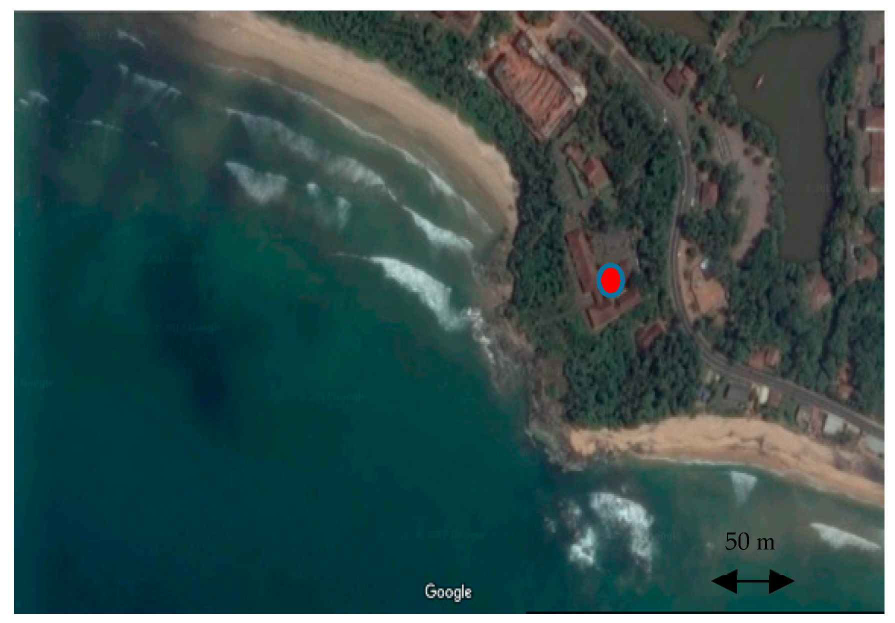
3. Experimental Setup

In this study, electric fields generated by lightning flashes were measured with a flat plate antenna system with a 30 MHz bandwidth, similar to the one used in reference [17]. The decay time constants of the measuring system were set to 1.0 s for the slow antenna and 15 ms for the fast antenna. The signals were recorded by a digitizer with 12-bit resolution. Data were recorded with a 6.4 ns sampling interval allowing a 200 ms sample window to be captured from a single trigger. The pre-trigger delay time was set to 60 ms. The bandwidth of the digitizer (PicoScope 6402B, Pico Technology co. ltd, St Neots, UK) was 250 MHz. The measurements were made at the southern coast (5.9360° N, 80.5738° E) of Sri Lanka during the south-west monsoon period of 2013 (see Figure 1). Most flashes occurred over the sea, so the path of propagation was over salt water, except for the last few tens of meters; hence, the propagation effect on the measured fields were minimal [18,19]. In this study, we have identified K-changes from the small step-like electrostatic field changes associated with them. This is the procedure through which Kitagawa [1] and Kitagawa and Kobayashi [2] first identified the K-changes. Since the electrostatic field decreases rapidly with distance, we could identify these step changes only in about 10% of the recorded flashes. The rest of the flashes probably occurred at distances where the radiation fields dominate the static fields. Out of a total of 1106 ground flashes analyzed, 98 flashes contained small static field changes that could be identified as K-changes. These ninety-eight flashes contained 165 K-changes.

The slow antenna system helped to identify the K-changes that occur as small steps in the static field change of the lightning flashes. Selected K-changes were used to measure the pulse train duration (T_K), the time interval between the first return stroke and K-change (T_RS1-K), the time to the next return stroke from the K-change (T_K-RS), and inter K-change interval (T_K-K). Figure 2 and Figure 3 illustrate the definition and the procedure of measuring the parameters mentioned above. Since the antennas are not calibrated at the site, the amplitudes of the recorded waveforms are given in volts.

Multiple K-changes taking place within a single inter-stroke time interval or after the final subsequent stroke were categorized as “Consecutive K-changes,” and if there was only one K-change for a particular flash or within a given inter-stroke time interval, it was categorized as an “Isolated K-change”. It is necessary to point out that the recording time window of the experiment is 200 ms, and it is possible that some of the late return strokes associated with lightning flashes that occur at times beyond this time window were missing in the recorded waveforms. However, since we have given the statistics corresponding to K-changes per return stroke, this drawback of the system would not significantly alter the statistics provided in the paper.

The Minitab^® statistical software (Minitab, Ltd., Coventry, UK) package was employed to conduct the statistical analysis. The goodness-of-fit test provided by the software package was used to identify the type of distribution at the 95% confidence interval.

4. Results

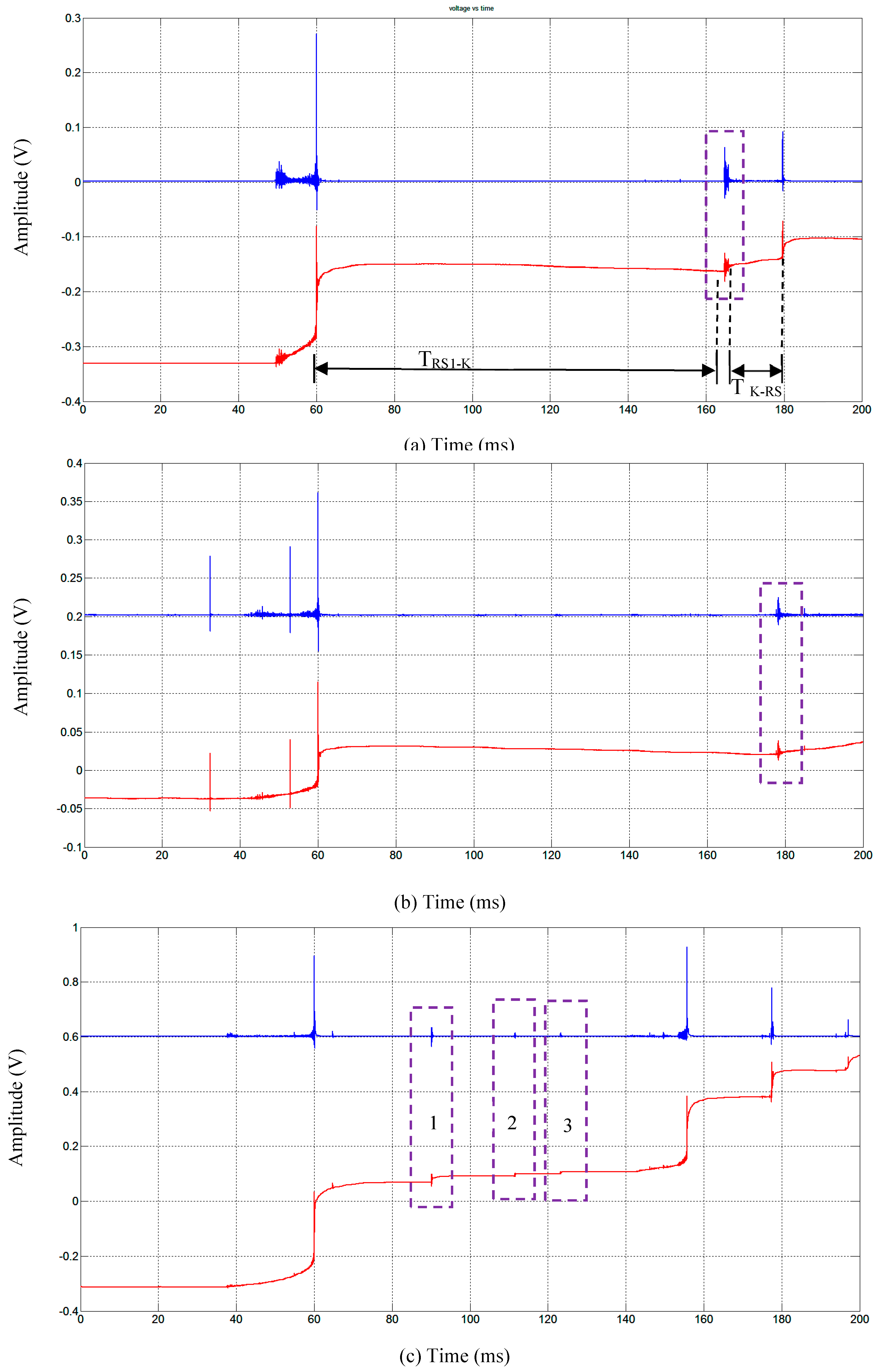
4.1. Characteristics of K-Changes

Table 1. Summary of selected K-changes for the analysis.

Total No. of Flashes	No. of Flashes with K-Changes	Total No. of K-Changes	No. of Flashes with Consecutive K-Changes	No. of Consecutive K-Changes	No. of Isolated K-Changes
1106	98	165	53	120	45

tabulates the number of K-changes belonging to different categories as observed in the present study. In this case, out of 1106 ground flashes, only 98 flashes contained clearly distinguishable K-changes. According to the observations, 53 flashes contained consecutive K-changes, and 45 flashes had isolated K-changes. In these 98 flashes, we found 165 K-changes. Thus, on average, there were about two K-changes per each flash. We also detected 204 return strokes in these 98 flashes. In the study conducted by Rakov et al. [8] in Florida, there were 263 K-changes in 46 ground flashes. That is, on average there were about six K-changes per flash which is significantly larger than the value observed in the present study. Note, however, that the two studies were conducted in different geographical regions, and the difference in the average number of K-changes per flash is caused probably by the differences in the lightning flash characteristics or the dimensions and height of charge centers in thunderclouds in the two regions.

Figure 2 presents a sample of isolated and consecutive K-changes. Note that the time zero of the records depicted in Figure 2 corresponds to the beginning of the recording window. Since there was a pre-trigger delay incorporated into the recording, the beginning of the window corresponds to a point 60 ms before the electric field feature that triggered the system.

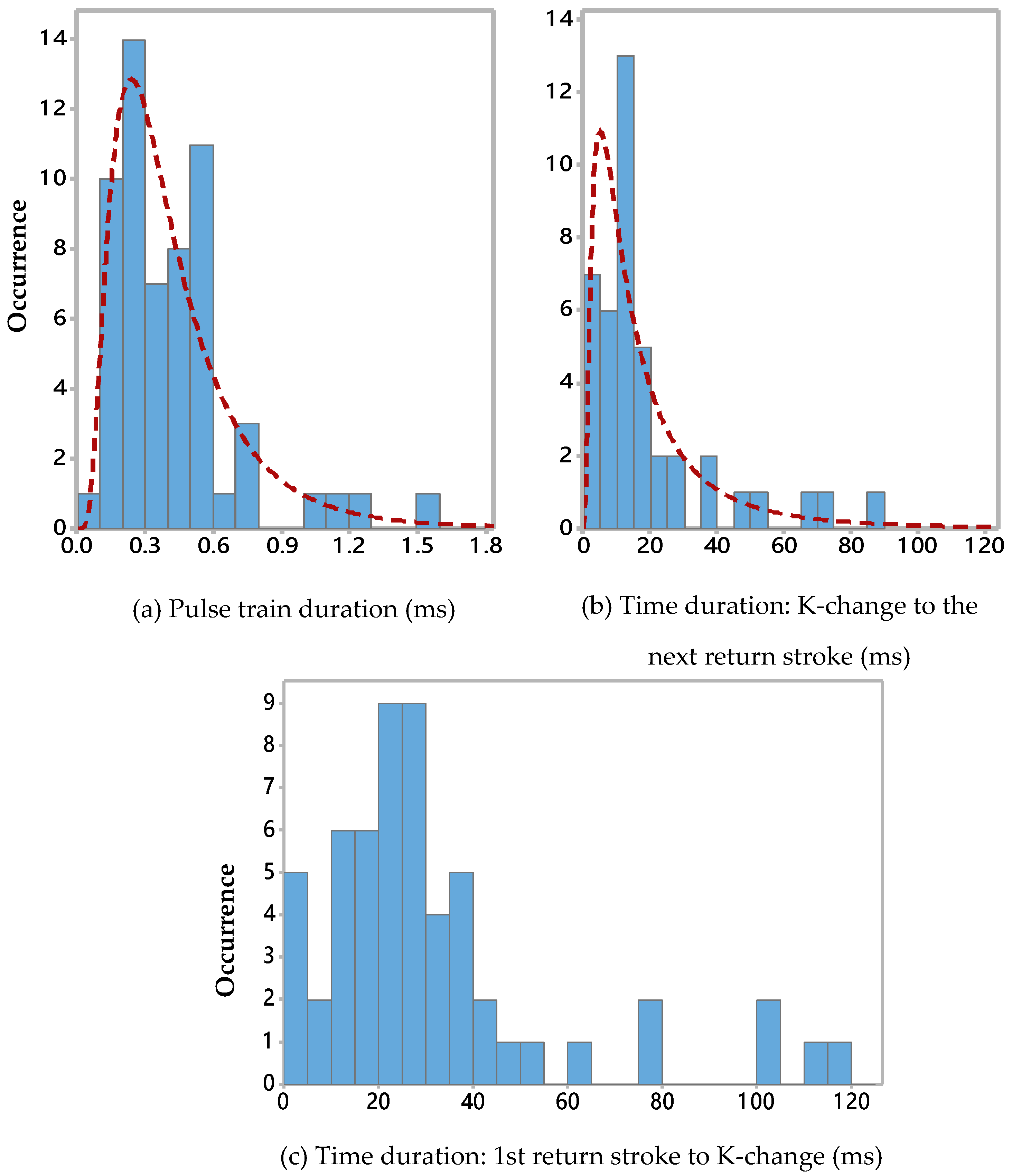
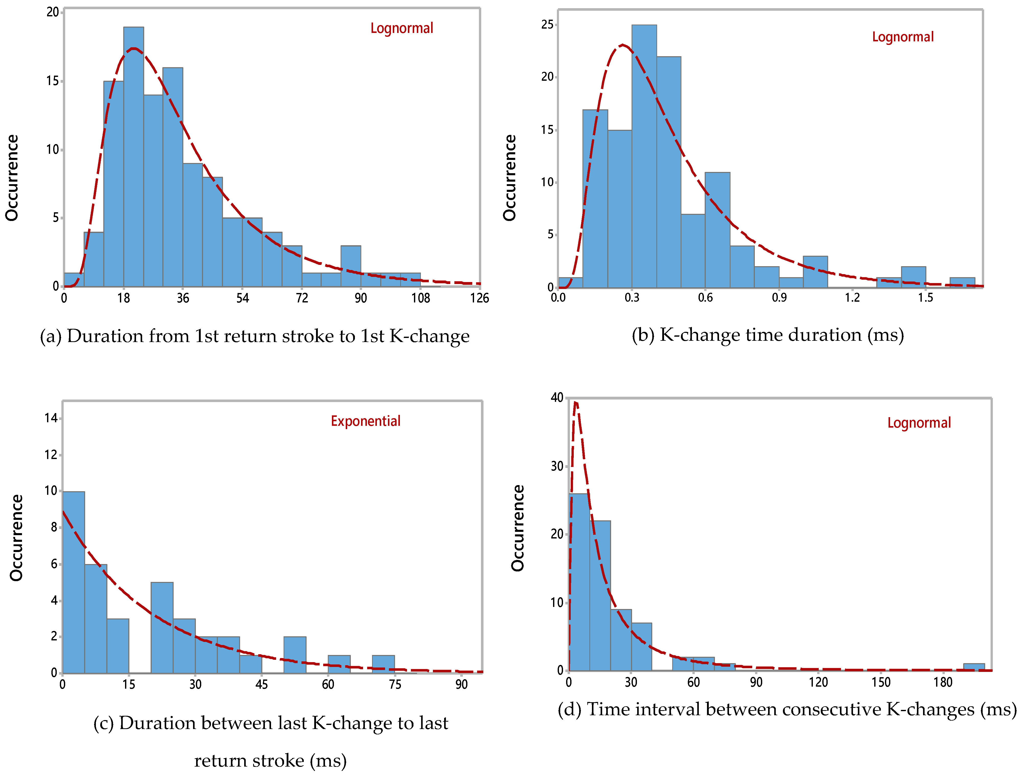
4.2. Parameters of Isolated K-Changes

Figure 4 presents the histograms of measured isolated K-change parameters. Accordingly, the histograms of T_K and T_K-RS have lognormal distributions, but the histogram of T_RS1-K does not fall into any of the provided distributions in the software package.

Table 2. Summary of the statistics for parameter distributions in Figure 4.

Parameter	Geometric Mean	St. Deviation	Minimum	Maximum	Typical Value
TK (ms)	0.43	0.3	0.08	1.599	0.2–0.3
TRS1-K (ms)	24.6	27.0	1.9	118.1	20–30
TK-RS (ms)	19.33	19.59	0.8	87.1	10–15

provides a summary of the statistical distributions in Figure 4, which indicates the geometric mean of the isolated K-change duration was around 0.43 ms, and the typical value (the bin value of the histogram where the peak of the distribution is observed) is 0.2–0.3 ms. According to Figure 4c, isolated K-changes are most likely to occur after 20–30 ms from the first RS.

4.3. Parameters of Consecutive K-Changes

As per Table 1, one-hundred-and-twenty consecutive K-changes were found in 53 ground flashes, and they were analyzed for T_K, time duration between starting RS to K-change of the consecutive order (T_RS-K), time interval between consecutive K-changes (T_K-K), and time duration between the last K-change of the consecutive order and ending RS (T_K-RS).

The histograms in Figure 5 denote the distribution of each of the measured parameters and their approximate distributions (without considering the K-change or RS order) provided by the software package.

Table 3. Summary of the statistics of the distributions in Figure 5.

Parameter	Average	Geometric Mean	Standard Deviation	Min.	Max.	Typical Value	Distribution
TR1-K1 (ms)	35.9	30.3	21.4	3.4	104.3	18–24	Lognormal
TK (ms)	0.45	0.38	0.29	0.045	1.65	0.3–0.4	Lognormal
TK-R (ms)	20.2	12.3	18.5	1.7	71.3	0–5	Exponential
TK-K (ms)	20.27	11.78	26.84	0.67	198.50	0–10	Lognormal

provides the statistical summary of the distributions in Figure 5, and

Table 4. Comparison of the results obtained for consecutive K-changes in the present study with the results obtained in previous studies. The mode range corresponds to the upper and lower limits of the histogram bin where the mode occurs.

Study	TK (ms)		TK-K (ms)			Distribution
	Geometric Mean	Typical Value	Average	Geometric Mean	Typical Value
(Kitagawa & Brook) [3]	-	-	8.50	-	4–6	Lognormal
(Kitagawa 1957) [1]	-	0.20–0.40	-	-	8–16	-
(Brook & Kitagawa 1964) [4]	-	0.50–0.75	-	-	-	-
(Thottapillil et al.) [20]	0.70	0.40–0.60	-	12.50	10–15	-
(Miranda et al.) [21]	-	-	18.50	12	10–16	Lognormal
This study	0.38	0.3 –0.4	20.27	11.78	0–10	Lognormal/Exponential

presents the comparison of the statistical values obtained for consecutive K-changes in this study with the results obtained by other researchers in previous studies for consecutive K-changes. It is important to note here that in general lightning parameters have lognormal distributions. In this respect, it is important to collect more data to check whether the exponential distribution in Figure 5c is a result of an insufficient amount of data.

Comparison of data tabulated in Table 3 and Table 4 signifies the geometric mean of T_K in the present study (0.38 ms) is much less than the value observed by early studies (0.7 ms). According to reference [7], the velocity of K-changes is in the order of a few times of 10⁷ m/s. This suggests that the length of the K-changes in our study is in the order of 5–10 km. This observation is consistent with K-changes being recoiled streamers which propagate along the channel of positive leaders cut off from their origin [6]. Although the typical range of T_K of the present study (0.3–0.4 ms) agrees with the value reported in study [20], the values reported by Kitagawa and Brook [3] and Thottapillile et al. [20] (i.e., 0.5–0.75, 0.4–0.6 ms) were higher than the values obtained in the present study. Comparing T_K-K denoted the average and geometric mean values (20.27 ms, 11.78 ms) of the present study closely agreed with those from the study by Miranda et al. [21] (i.e., 18.5 ms, 12 ms), although histograms follow different distributions. It is essential to re-emphasize that the discharge processes associated with K-changes are probably controlled by the size and height of the charge centers. Since these parameters may differ in thunderclouds in different geographical locations, one may expect the K-change parameters to differ in diverse geographic regions.

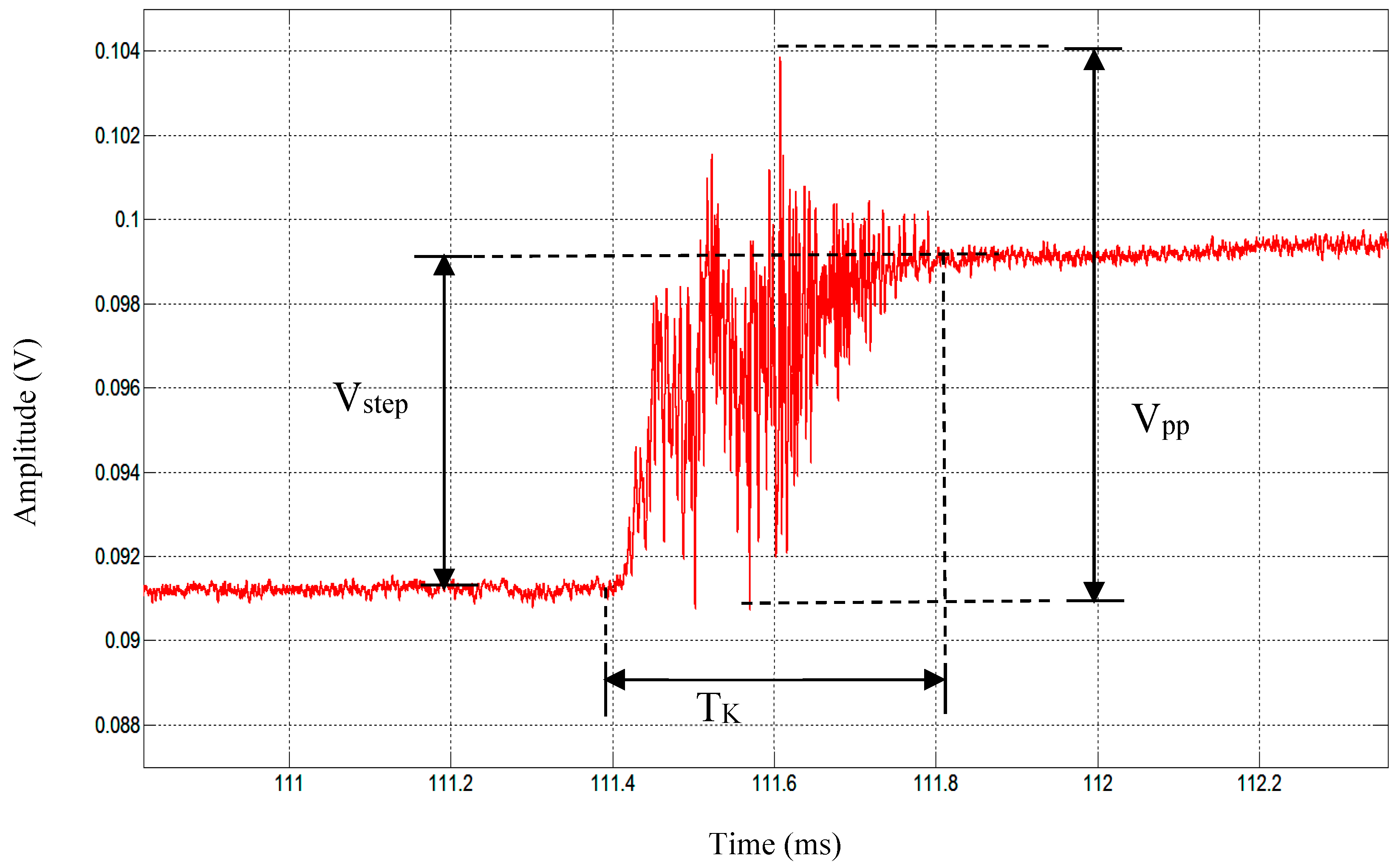
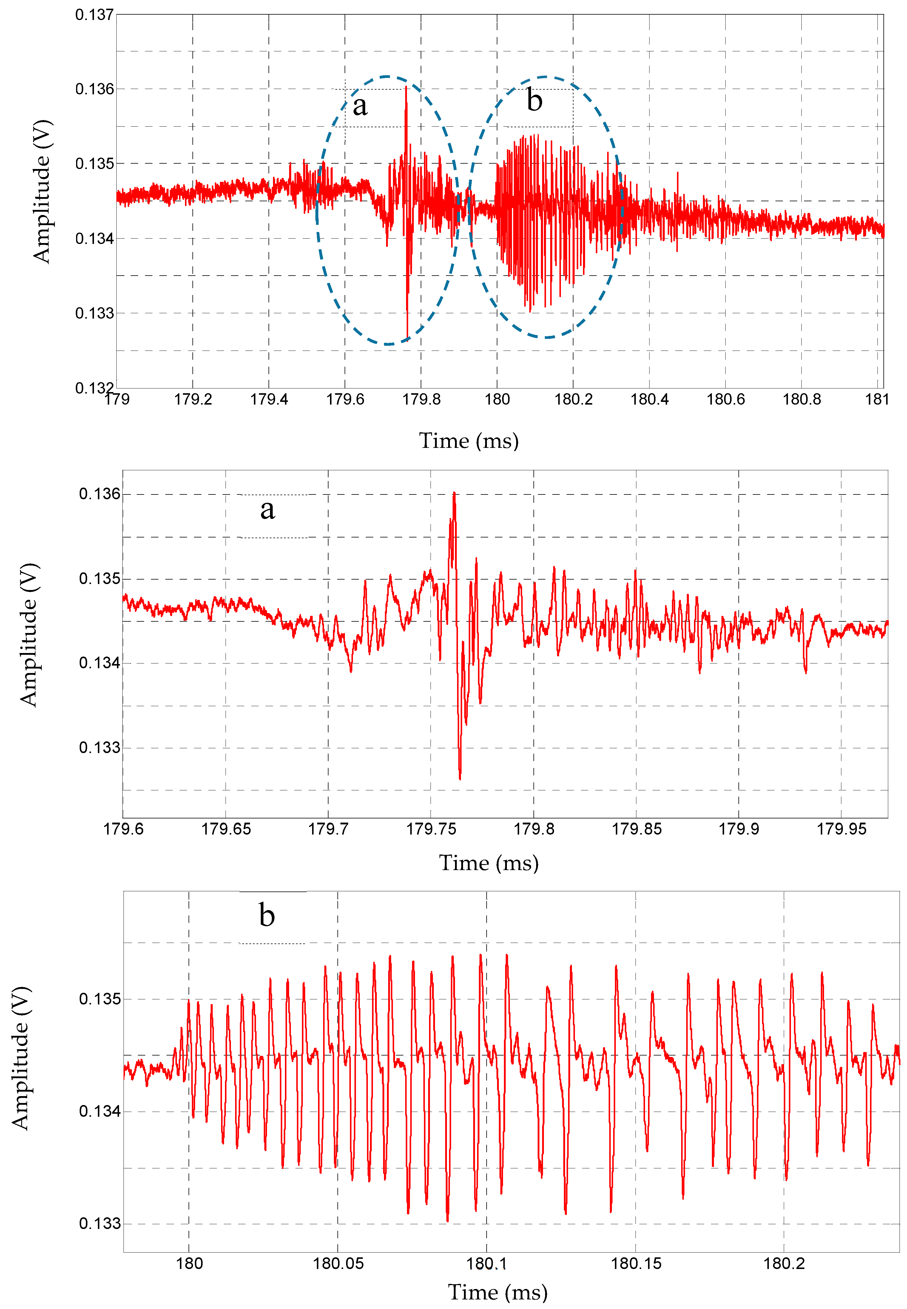
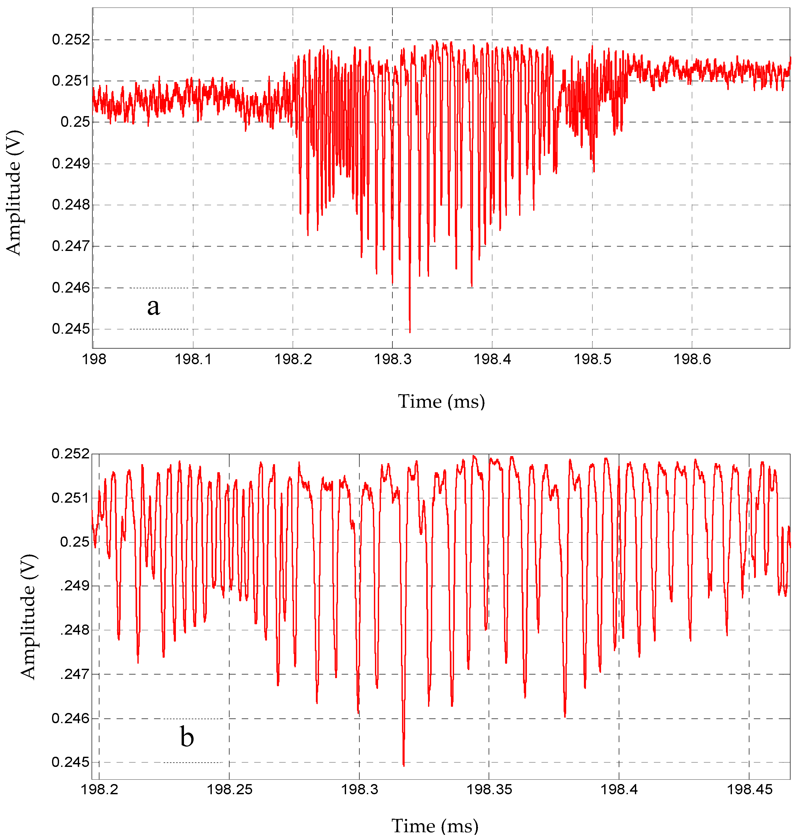
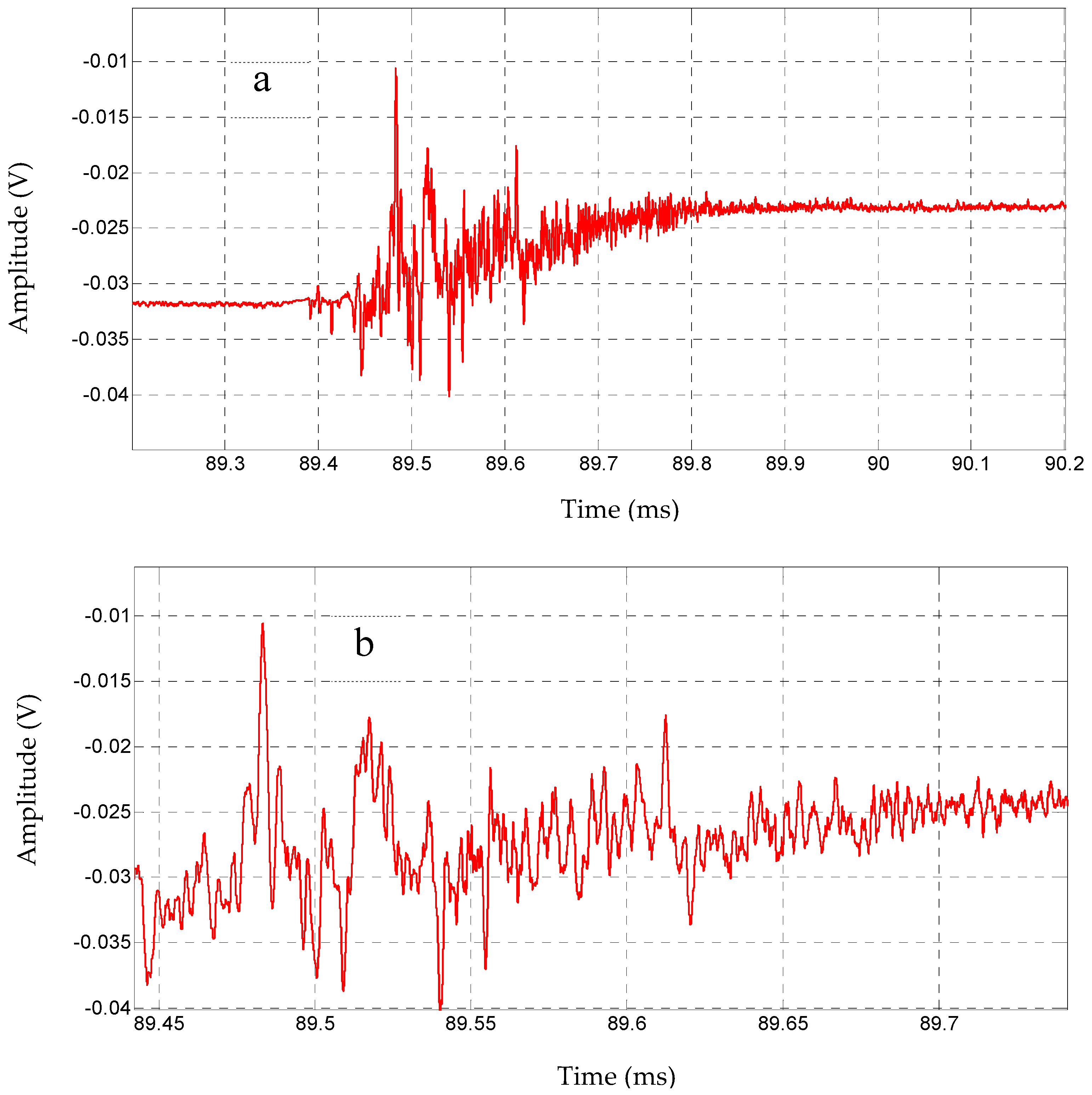
4.4. Fine Structure of K-Change Electric Fields

The appearance of the static field of the K-change process in the recording system highly depends on measuring system bandwidth, sensitivity, the sampling rate of the recording system, and the distance to the lightning flash from the measuring station [2]. It was pointed out in [20] that using antenna system decay time constants of 0.3 ms and 3 ms were insufficient to record the static field changes without distortion. If the decay time constant of the antenna system is too small, the step-like (or ramp-like) static field changes of K-changes may appear as a pulse with a certain rise time and decay time.

Several examples of the typical slow wave shapes of K-changes from the present study are depicted in Figure 2, and the fine structure associated with it is illustrated in Figure 3 and Figure 6, Figure 7, Figure 8 and Figure 9. As can be seen, the overall K-change wave shape (or the static field change) presents a characteristic ramp or step-like behavior when measured using a slow antenna. Similar observations have been reported in Figure 2c of study [22] although they have not explicitly mentioned the wave shape. Indeed, Kitagawa [1] and Kitagawa and Kobayashi [2] identified these static field changes as K-changes because they lacked sufficient resolution in their measurements at that time to visualize the radiation field pulses superimposed on the static field change.

Previously, Rakov et al. [8,9] studied the fine structure associated with K-changes (and also M-changes). However, the time resolution of the present study is much better than the time resolution of the data available to Rakov et al. [8,9]. Hence, more details of the fine structure can be observed here. Our study designates the overall static field wave shape of K-changes can be described as a ramp or a step-change with superimposed micro-second scale radiation field pulses that start at the beginning of the K-change, and last almost during the total duration of the K-change, as illustrated in Figure 3. Our study indicates the fine structure associated with the K-change is either a chaotic pulse train (CPT) or a combination of chaotic and regular pulse trains (RPT). This fine structure starts at the beginning of the K-change and continues almost to the end of the K-change. Indeed, all the K-changes observed in our study are associated with CPTs or a combination of CPTs and RPTs.

Observe also that the individual pulses in pulse trains occasionally appear almost unipolar and in some cases, purely bipolar. This difference is probably associated with the differences in the way in which the current and the velocity of the discharge processes that generated these pulses vary in space and time.

As pointed out earlier, Ismail et al. [16] made a detailed analysis of chaotic pulse trains and observed that they could start or end as regular pulse trains. Sometimes the regular pulse trains occur in the middle of the chaotic pulse train. Based on their investigation that consists of both experiment and numerical simulations, they concluded that chaotic pulse trains are produced by a random superposition of regular pulse trains. They pointed out that several dart-stepped like leaders, each producing a regular pulse train, propagating in random directions concerning each other, could give rise to a chaotic pulse train. This hypothesis could explain why some of the chaotic pulse trains either start or end as regular pulse trains. In this study, we observed that K-changes are associated with either a chaotic pulse train or a combination of the chaotic pulse train and regular pulse trains (see Figure 3 and Figure 6, Figure 7, Figure 8 and Figure 9). Observation of this study, as shown in Figure 6, Figure 7, Figure 8 and Figure 9, agree with the hypothesis of Ismail et al. [16].

Figure 3 and Figure 6, Figure 7, Figure 8 and Figure 9 illustrate the electrostatic field change of the K-change is produced by the physical activity in the cloud that gives rise to either chaotic pulse train or a combination of chaotic and regular pulse trains (or as pointed out by Ismail et al. [16] to a random superposition of regular pulse trains). It is vital to realize that the fast pulses associated with the CPTs and RPTs are essentially radiation, probably at distances as close as a few kilometers. This is the case because the duration of the individual pulses lies in the microsecond scale and a distance of a few kilometers is much longer than the typical wavelength of about 300 m or so associated with these pulses. However, the static field caused by the charge transfer associated with the physical process that generates these radiation field pulses may appear as a step field change on which the radiation field pulses are superimposed (see Figure 3 and Figure 9a). The amplitude of the static step will increase as the thunderstorm that generated the K-change becomes closer to the measuring station, and at close distances, the static field can dominate the radiation fields. In such cases, if a K-change is measured by an antenna without high time resolution, then the K-change may appear as an electrostatic field step or a ramp. Thus, it is reasonable to state that the small static field changes categorized by Kitagawa and Kobayashi [2] as K-changes are actually the static field changes associated with the chaotic pulse trains or a combination of chaotic and regular pulse trains.

As mentioned earlier, Weidman [14] first observed the chaotic pulse trains to be associated with subsequent return strokes. Observations in this study suggest that the K-changes are associated with chaotic pulse trains. According to the observations of Shao et al. [7], there is no physical difference between the processes that initiate subsequent strokes, K-changes, and M components. All of these different processes are associated with negative discharges originating at the ends of the cut-off points of positive channels and propagating towards the point of origin of the return strokes [6]. If the discharge happens to make contact with a hot and low dense lightning channel, it will lead to a dart leader that will end-up as a subsequent stroke. If the discharge makes contact with a lightning channel through which a continuous current is flowing, it will end up as an M component.

Conversely, if the discharge ends up on a defunct lightning channel where the temperature has decayed (and hence the density is restored) to such an extent that a current through which could not be ignited during the encounter, the process will appear as a K-change. The results presented here in combination with Shao’s findings indicate that the fine structure associated with M components may also consist of chaotic pulse trains. Indeed, Rakov et al. [8] discovered radiation field pulses embedded in the static field of M components. However, the time resolution of their measurements was not adequate to identify and categorize these radiation field pulses.

5. Conclusions

This paper presented a detailed analysis of the K-change characteristics and associated chaotic pulse trains observed in Sri Lanka, in the tropics. We observed that, on average, about two K-changes occurred in each lightning flash. The mean K-change time duration observed in this study is 0.38 ms. Assuming that the speed of the K-changes is a few times of 10⁷ m/s, this time duration suggests that the length of K-change activity may be in the order of 5–10 km. The study reveals that the fine structure associated with the K-change is either a chaotic pulse train or a combination of chaotic and regular pulse trains. In this respect, one can conclude that the small static field changes, identified initially by Kitagawa [1] and Kitagawa and Kobayashi [2] as K-changes, are the step-like static field changes associated with the physical processes that induce the radiation field pulses known as chaotic and regular pulse trains. Thus, at larger distances where the static fields can be neglected, the K-changes may appear as a chaotic or a combination of chaotic and regular pulse trains.

References

1. Kitagawa, N. On the mechanism of cloud flash and junction or final process in flash to ground. Pap. Meteorol. Geophys. 1957, 7, 415–424. [Google Scholar] [CrossRef]
2. Kitagawa, N.; Kobayashi, M. Field Changes and Variations of Luminosity due to Lightning Flashes in Recent Advances in Atmospheric Electricity; Smith, L.G., Ed.; Pergamon: Oxford, UK, 1959; pp. 485–501. [Google Scholar]
3. Kitagawa, N.; Brook, M.A. Comparison of intracloud and cloud-to-ground lightning discharges. J. Geophys. Res. 1960, 65, 1189–1201. [Google Scholar] [CrossRef]
4. Brook, M.; Kitagawa, N. Radiation from lightning discharges in the frequency range 400 to 1000 Mc/s. J. Geophys. Res. 1964, 69, 2431–2434. [Google Scholar] [CrossRef]
5. Ogawa, T.; Brook, M. The mechanism of the intracloud lightning discharge. J. Geophys. Res. 1964, 69, 5141–5150. [Google Scholar] [CrossRef]
6. Mazur, V.; Ruhnke, L.H.; Warner, T.A.; Orville, R.E. Recoil leader formation and development. J. Electrostat. 2013, 71, 763–768. [Google Scholar] [CrossRef] [Green Version]
7. Shao, X.M.; Krehbiel, P.R.; Thomas, R.J.; Rison, W. Radio interferometric observations of cloud-to-ground lightning phenomena in Florida. J. Geophys. Res. 1995, 100, 2749–2783. [Google Scholar] [CrossRef]
8. Rakov, V.A.; Thottappillil, R.; Uman, M.A. Electric field pulses in K and M changes of lightning ground flashes. J. Geophys. Res. 1992, 97, 9935–9950. [Google Scholar] [CrossRef]
9. Rakov, V.A.; Uman, M.A.; Hoffman, G.R.; Masters, M.W.; Brook, M. Bursts of pulses in lightning electromagnetic radiation observations and implications for lightning test standards. IEEE Trans. 1996, 38, 156–164. [Google Scholar] [CrossRef]
10. Krider, E.P.; Radda, G.J.; Noggle, R.C. Regular radiation field pulses produced by intracloud lightning discharges. J. Geophys. Res. 1975, 80, 3801–3804. [Google Scholar] [CrossRef]
11. Wang, Y.; Zhang, G.; Zhang, T.; Li, Y.; Zhao, Y.; Zhang, X.; Wu, B. The Regular Pulses Bursts in Electromagnetic Radiation from Lightning; APEMC: Beijing, China, 2010. [Google Scholar]
12. Davis, S.M. Properties of Lightning Discharges from Multiple Station Wideband Measurements. Ph.D. Thesis, University of Florida, Gainesville, FL, USA, 1999. [Google Scholar]
13. Kolmasová, I.; Santolík, O. Properties of unipolar magnetic field pulse trains generated by lightning discharges. Geophys. Res. Lett. 2013, 40, 1637–1641. [Google Scholar] [CrossRef] [Green Version]
14. Weidman, C.D. The Sub-Microsecond Structure of Lightning Radiation Fields. Ph.D. Thesis, University of Arizona, Tucson, AZ, USA, 1982. [Google Scholar]
15. Gomes, C.; Cooray, V.; Fernando, M.; Montano, R.; Sonnadara, U. Characteristics of chaotic pulse trains generated by lightning flashes. J. Atmos. Sol. Terr. Phys. 2004, 66, 1733–1743. [Google Scholar] [CrossRef]
16. Ismail, M.M.; Rahman, M.; Cooray, V.; Fernando, M.; Hettiarachchi, P.; Johari, D. On the Possible Origin of Chaotic Pulse Trains in Lightning Flashes. Atmosphere 2017, 8, 29. [Google Scholar] [CrossRef]
17. Galvan, A.; Fernando, M. Operational Characteristics of a Parallel-Plate Antenna to Measure Vertical Electric Fields from Lightning Flashes; Uppsala University: Uppsala, Sweden, 2000; pp. 2–17. [Google Scholar]
18. Ye, M.; Cooray, V. Propagation effects caused by a rough ocean surface on the electromagnetic fields generated by lightning return strokes. Radio Sci. 1994, 29, 73–85. [Google Scholar]
19. Cooray, V.; Ye, M. Propagation effects on the lightning-generated electromagnetic fields for homogeneous and mixed sea land paths. J. Geophys. Res. 1994, 99, 10641–10652. [Google Scholar] [CrossRef]
20. Thottappillil, R.; Rakov, V.A.; Uman, M.A. K and M changes in close lightning ground flashes in Florida. J. Geophys. Res. 1990, 95, 18631–18640. [Google Scholar] [CrossRef]
21. Miranda, F.J.; Pinto Jr, O.; Saba, M.M.F. A study of the time-interval between return strokes and K-changes of negative cloud-to-ground lightning flashes in Brazil. Atmos. Sol. Terr. Phys. 2003, 65, 293–297. [Google Scholar] [CrossRef]
22. Stolzenburg, M.; Marshall, C.M.; Karunarathne, S.; Karunarathna, N.; Warner, T.A.; Orville, R.E. Stepped-to-dart leaders preceding lightning return strokes. J. Geophys. Res. 2013, 118, 9845–9869. [Google Scholar] [CrossRef] [Green Version]
Figure 1. A satellite view of the measuring station (red dot) located in a few tens of meters from the sea. Adapted from Google maps (10/ 9/ 2017). Imagery ©2017 DigilatGlobe, Map data ©2017 Google.
Atmosphere 10 00141 g001
Figure 2. (a) Isolated K-change between two return strokes, (b) Isolated K-change occurred after the last return stroke captured inside the recording time window, and (c) Three consecutive K-changes. Electric fields recorded using fast and slow antenna systems are presented in blue and red colors. Measured parameters of TRS1-K and TK-RS are presented in (a) above. Data were recorded on 4/3/2013 19:53:00. UTC.
Atmosphere 10 00141 g002
Figure 3. First K-change in Figure 2c in an expanded time-scale presenting the measured parameters of TK, Vstep, and Vpp. The signal was recorded by the slow antenna system.
Atmosphere 10 00141 g003
Figure 4. Histogram of the isolate K-change measured parameters: (a) TK (duration of K-change pulse train), (b) TK-RS, (c) TRS1-K. The red dotted line represents the lognormal distribution for the histograms in figures (a,b). Data in Figure (c) do not fit into any of the distributions provided by the software package.
Atmosphere 10 00141 g004
Figure 5. Histograms of the measured parameters of consecutive K-changes: (a) TRS1-K1, (b) TK, (c) TK-RS, and (d) TK-K. Histograms (a,b,d) Follow Lognormal distribution while (c) follows an Exponential distribution. The dotted red lines indicate the assigned distributions.
Atmosphere 10 00141 g005
Figure 6. K-change starting with a chaotic pulse train and ending with a regular pulse train circled in dotted blue lines. Figures (a,b) shows the expanded view of chaotic and regular pulse components. Data were recorded on 5/5/2013 08:04:00. UTC.
Atmosphere 10 00141 g006
Figure 7. K-change starting with a chaotic pulse train (or somewhere between a chaotic and regular train) and ending with a regular pulse train (circled in dotted blue lines). Figures (a,b) shows the expanded view of chaotic and regular pulse components. Data were recorded on 4/5/2013 20:06:00. UTC.
Atmosphere 10 00141 g007
Figure 8. (a) K-change consists of a regular pulse train probably followed by a chaotic pulse train, (b) Expanded view of the regular pulses. Data were recorded on 4/5/2013 20:08:00. UTC.
Atmosphere 10 00141 g008
Figure 9. (a) K-change consists of a chaotic pulse train, (b) Expanded view of the chaotic pulses. Data were recorded on 4/5/2013 20:06:00. UTC.
Atmosphere 10 00141 g009