Article

Impacts of Onset Time of El Niño Events on Summer Rainfall over Southeastern Australia during 1980–2017

South China Sea Institute of Marine Meteorology, College of Ocean and Meteorology, Guangdong Ocean University, Zhanjiang 524088, China
*
Author to whom correspondence should be addressed.
Atmosphere 2019, 10(3), 139; https://doi.org/10.3390/atmos10030139
Submission received: 21 January 2019 / Revised: 23 February 2019 / Accepted: 7 March 2019 / Published: 14 March 2019

Abstract

:
El Niño–Southern Oscillation (ENSO) has large impacts on Australia’s rainfall. A composite analysis technique was utilized to distinguish the impact of onset time of El Niño on summer rainfall over southeastern Australia. Summer rainfall tended to be lower than normal in austral autumn El Niño events during December–January–February (DJF) and higher than normal in austral winter El Niño events, in 1980–2017. During autumn El Niño events, the Walker circulation and meridional cells served as a bridge, linking the warmer sea surface temperature (SST) in the eastern equatorial Pacific (EEP) and lower summer rainfall over southeastern Australia. This physical process can be described as follows: During DJF, a positive SST anomaly in the EEP was concurrent with anomalous downdraft over southeastern Australia via zonal anomalous Walker circulation, meridional anomalous cells along 170° E–170° W, and a Pacific South American (PSA) teleconnection wave train at 500 hPa. In addition, an anomalous convergence at 200 hPa depressed the convection. Meanwhile, an 850 hPa abnormal westerly was not conducive to transport marine water vapor into this area. These factors resulted in below-normal rainfall. During winter El Niño events, a positive SST anomaly in the central equatorial Pacific (CEP) and the changes in Walker circulation and meridional cells were weaker. The PSA teleconnection wave train shifted westward and northward, and there was a low-level anomalous ascent over southeastern Australia. At the western flank of the anomalous anticyclone, northerly transported water vapor from the ocean to southeastern Australia resulted in a sink of water vapor over this area. The development of low-level convective activity and the plentiful water vapor supply favored more rainfall over southeastern Australia. Onset time of El Niño may be a useful metric for improving the low predictive skill of southeastern Australian summer rainfall.

1. Introduction

Rainfall in different parts of Australia is highly variable [1]. Southeastern Australia is a highly populated region and provides for a large portion of Australia’s agricultural production [2], so rainfall variability in this area has a substantial impact from a variety of perspectives. Most previous studies have focused on winter rainfall in southern Australia because of its large impacts on ecosystem performance and societal development [2,3]. In contrast, summer rainfall attracts less attention, despite extreme summer rainfall being capable of causing severe disasters. For example, in December 1982 to February 1983, a very strong El Niño impact on subtropical eastern Australia with drought conditions widespread across eastern and southern Australia, which resulted in farm losses of a thousand million dollars, and undoubtedly contributed to the Ash Wednesday disaster [4]. Flood in southeastern Australia is frequent in summer. In Australia this was never more apparent than in January 2011 when widespread flooding across Queensland, New South Wales (NSW), and Victoria resulted in the loss of human lives and devastating impacts to infrastructure and local economies [5,6,7]. Thus, exploring the sources of predictability, and making skillful rainfall forecasts of southeastern Australia summer rainfall will have economic and societal significance.
Air–sea interactions occurring over the southern high latitudes form a complex system [3]. El Niño–Southern Oscillation (ENSO) [8,9,10,11,12], Indian Ocean Dipole (IOD) [13,14], ENSO + IOD [15,16,17], Interdecadal Pacific Oscillation (IPO) [18], and the Southern Annular Mode (SAM) [19,20,21,22] are documented as having influences on precipitation in Australia. Southeastern Australia is influenced by combined ENSO, IOD, and SAM interactions [23]. This study only focuses on ENSO.
ENSO is the most dominant interannual signal of climate variability on Earth [24,25] and has large impacts on Australian rainfall [8,26]. It has been suggested that over interannual time scales, ENSO acts as a primary driver of subtropical eastern Australian rainfall [27], as abnormally low precipitation tends to appear during El Niño episodes [8]. However, after the 1980s, the relationship between ENSO strength and Australian summer rainfall was insignificant [28] and the seasonal forecast skill of Australia summer rainfall turned out to be quite low [29]. The low predictive skill of southeastern Australia summer rainfall (SASR) inspires us to revisit this relationship. Is there another metric in the ENSO–SASR relationship during 1980–2017?
The evolution of ENSO may have different flavors [30,31,32,33,34,35]. The diversity in patterns, amplitude, and temporal evolution of ENSO will be referred to as its complexity [36]. Previous studies have advanced our understanding of the relationship of ENSO with rainfall over southeastern Australia. Brown et al. [37] showed that different patterns of El Niño (canonical and Modoki) have different impacts on southeastern Australia rainfall. Classified by the onset time of sea surface temperature (SST)anomalies, El Niño can be distinguished into a boreal spring or summer type [35], that is, austral autumn or winter flavor. So far, no studies have linked SASR to variability in the onset time of El Niño events. Thus, it remains unclear how SASR variability manifests itself, or whether and how it is linked to different onset times of El Niño events. If it does, how are they related and what is the underlying mechanism? In this study, we attempt to address these questions. If we get some useful information, we can predict SASR in two or three seasons ahead of time.
The remainder of this manuscript is organized as follows: A brief description of data and methodology is shown in Section 2. The classification of El Niño events and the climatic characteristics of SASR are documented in Section 3. The influence of El Niño events on rainfall and other atmospheric variables is described in Section 4. Section 5 presents a summary of our findings.

2. Data and Methods

2.1. Data

The datasets employed in this study are summarized as follows: Monthly precipitation records of 325 meteorological stations were obtained from the Australian Bureau of Meteorology (http://www.bom.gov.au/climate/data/) from the beginning of data availability through to 2017. The monthly COBE SST (Centennial in situ Observation Based Estimates of the variability of SST) data were obtained from NOAA (https://www.esrl.noaa.gov/psd/), representing 1891 to present, gridded on a 1.0° × 1.0° mesh [38]. The atmospheric monthly mean data (winds, specific humidity, and geopotential height) were provided by the NCEP–NCAR (http://www.esrl.noaa.gov/psd/data/gridded/data.ncep.reanalysis.html) reanalysis dataset [39], with a resolution of 2.5° × 2.5° grid. The monthly outgoing longwave radiation (OLR) data, with horizontal grid spacing of 2.5°, longitude and latitude, was provided by NOAA’s National Climatic Data Center (http://www.ncdc.noaa.gov) [40]. The monthly oceanic Niño index was provided by NOAA’s Climate Prediction Center (http://origin.cpc.ncep.noaa.gov/products/analysis_monitoring/ensostuff/ONI_v5.php), which is defined as a three-month running mean of SST anomalies over five consecutive months in the Niño 3.4 region of (5° S–5° N, 120°–170° W).
The austral seasons in the study area are grouped as: Spring (September–November), summer (December–February), autumn (March–May), and winter (June–August). The subtropical region of southeastern Australia refers to the region (25°–44° S and 136°–155° E). Summer (December–January–February, DJF) rainfall is defined as the average of rainfall in this region.

2.2. Methods

All datasets used in this study covered the period 1979–2016. The daily and monthly data obtained from different sources (described above) were summed (for precipitation) or averaged (for SST, wind, and OLR) into seasonal time series. These seasonal time series were then used to calculate seasonal anomaly time series for correlation and composite analysis.
The relationships between pairs of variables were examined by correlation or composite analysis and the statistical significance of these analyses were assessed using the two-sided Student’s t-test [41].

2.3. El Niño Event Classification

The SST anomaly averaged over the Niño 3.4 region of (5° S–5° N, 120° W–170° W,) was taken as an ENSO index (because it is better than other indexes in the present study). An El Niño phase was defined as three-month running mean of SST anomalies in the Niño 3.4 region which exceeded 0.5 °C for a minimum of five consecutive overlapping three-month seasons.
The onset time of El Niño was defined as the month just before the month when the SST anomaly first exceeded 0.5 °C. Austral autumn El Niño events began in months between February and May, and winter events in months between June and September. The treatment of breakpoints was as follows: If the index (≥0.5 °C) had a break of two months or more, the two events were considered discontinuous. If the index (≥0.5 °C) was interrupted for only one month, and the three-month running average of them exceeded 0.5 °C, the event was continuous; otherwise, it was considered discontinuous [41].
Based on the above definition, there were five austral autumn (February–May) El Niño events (1982/83, 1991/92, 1997/98, 2002/03, 2015/16) and four austral winter (June–September) El Niño events (1986/88, 1994/95, 2004/05, 2009/10) during 1980–2017 (Table 1). Figure 1 shows that the austral autumn El Niño events, with an average duration of 13 months and an average amplitude of 1.24 °C, were strong warm events of long duration. Austral winter El Niño events, with an average duration of 9 months and an average amplitude of 0.89 °C, were weak warm events of short duration. Furthermore, the maximum anomaly for both types occurred in November–January, which implies that the mature phase of El Niño events is highly phase-locked with the seasonal cycle, irrespective of the onset time [35,36,41]. We also investigated the relationship between start time and intensity of El Niño events in the following DJF Niño 3.4 index, one by one (figures omitted). There was a close relationship between them. Autumn El Niño was often strong, while winter El Niño was often weak.

3. Results

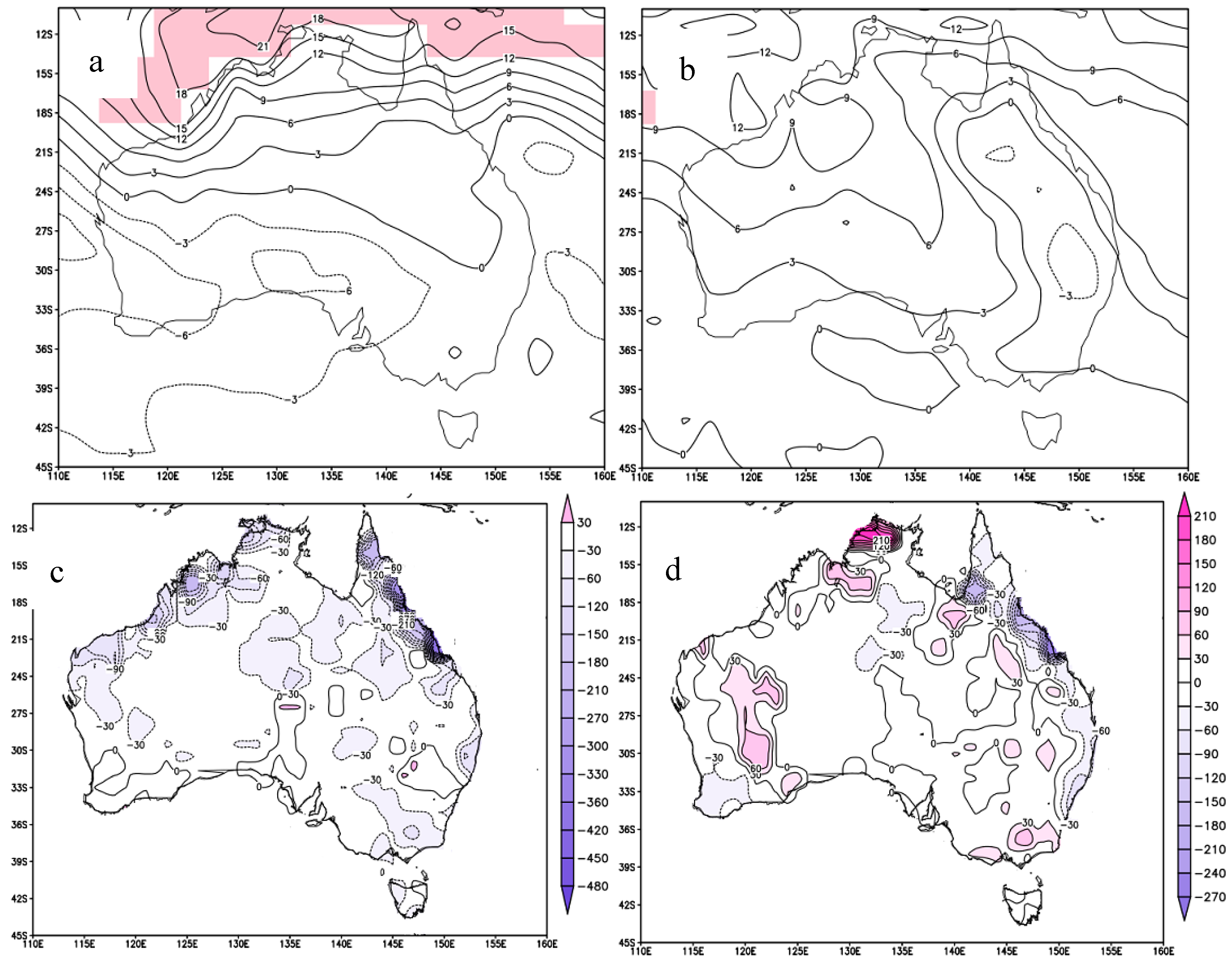
3.1. Climatic Characteristics of Summer Precipitation over Subtropical Southeastern Australia

The summer rainfall amounts ranged from 100 mm to 400 mm over subtropical southeastern Australia, were less than 200 mm over central and western Australia, and more than 400 mm over northern Australia (Figure 2a). In the present study, we focused on subtropical southeastern Australia, non-monsoon area, where the summer rainfall amount was 100–400 mm and accounted for 20–40% of the annual total rainfall (Figure 2b). The correlation coefficients between the DJF Niño 3.4 index and SASR anomalies were calculated. Results indicate that the relationship between them experienced an interdecadal change around the 1980s. During 1956–1979, the correlation coefficient between them was −0.41, passing the 95% confidence level. In contrast, this correlation then dropped dramatically (−0.08) and was insignificant during 1980–2017. This may be the reason that the seasonal forecast skill of Australian summer rainfall turned out to be quite low [29]. No significant linear correlation is detected, seemingly indicating that ENSO has no contribution to SASR. We note, however, that only the linear part of such a relationship can be detected in correlation analysis. To avoid overlooking a possible nonlinear relationship and improve the seasonal forecast skill of SASR during 1980–2017, the temporal evolution of the Niño 3.4 SST anomaly and relative deviations of SASR during DJF 1980–2017 is shown in Figure 3. Figure 3 shows that SASR in austral winter El Niño events was much higher than normal. Positive relative deviations of SASR occurred in periods of weaker winter El Niño events, such as 1994/95, 2004/05 and 2009/10, which associated with the positive or neutral southern annular mode (SAM). While 1986/88 negative SAM [42] was responsible for the decreased SASR, a positive SAM can mean that more easterly winds bring moist air from the Tasman Sea and hence increase rain as the winds hit the southeastern coast [20]. However, for the austral autumn El Niño events, negative relative deviations of SASR occurred in periods of stronger autumn El Niño events, such as 1982/83, 1997/98, 2002/03, and 2015/16, and another event (1991/92) had a positive anomaly. The positive 1991/1992 El Niño summer rainfall anomaly may be influenced by the Indian Ocean Dipole (IOD) (1992 was in a negative IOD phase; the others were in a positive or neutral phase [43]) more than the impact of El Niño onset time. A negative IOD typically results in above-average rainfall over parts of southern Australia [44] because, in addition to ENSO, the southeastern Australia climate is driven by IOD and SAM [45]. Each of these drivers could be expected to alter the structure of synoptic systems over Australia and hence rainfall. It is worth noticing that the number of events (five autumn and four winter El Nino) is too limited, so the statistical significance will be verified in the future.

3.2. Possible Mechanism of the Rainfall Differences between Autumn and Winter El Niño Events

To untangle the difference in the relationship between SASR and the two flavors of El Niño events, the tropical ocean SST, atmospheric circulation, and water vapor transport differences between austral autumn El Niño events and winter El Niño events were explored.

3.2.1. Composite Analysis for the Pacific SST Variability
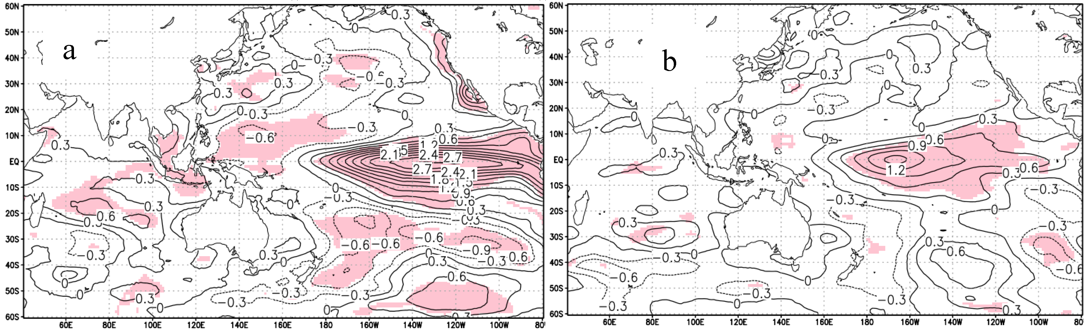
Large-scale SST variability can exert strong impacts on climate, as the ocean is the important heat sink of the climate system. Figure 4 reveals the spatial structures of the El Niño-related SST anomalies in DJF (mature phase of El Niño) for austral autumn and winter El Niño events separately, from which we can see significant differences:
(1)
In the autumn El Niño events, significant positive SST anomalies in the eastern equatorial Pacific (EEP) were larger, with the maximum anomaly 2.7 °C located within 120–140° W. A wide area of positive SST anomalies stretched southeastward from the eastern tropical Indian Ocean to Australia, and a considerable zone of positive SST anomalies covered the east of Australia. There are two significant negative anomaly zones in the Pacific Ocean. The northern branch extended northeastward from the Philippine Sea to the North Pacific, with a maximum value of −0.6 °C. The stronger southern branch stretching from New Zealand to South America along 30–40° S, with a wide-area maximum value of −0.9 °C;
(2)
In the winter El Niño events, the maximum anomaly was only 1.5 °C and in the central equatorial Pacific (CEP, within 160–170° W), exhibited weaker and smaller spatial scales than those during autumn El Niño. At the same time, the two negative anomaly branches in the Pacific Ocean all weakened and covered smaller areas, and negative SST anomalies were closer to Australia’s southeastern coast. The zonal and meridional gradient of SST in the Pacific were weaker in the winter El Niño events compared to their counterpart—in a normal year.

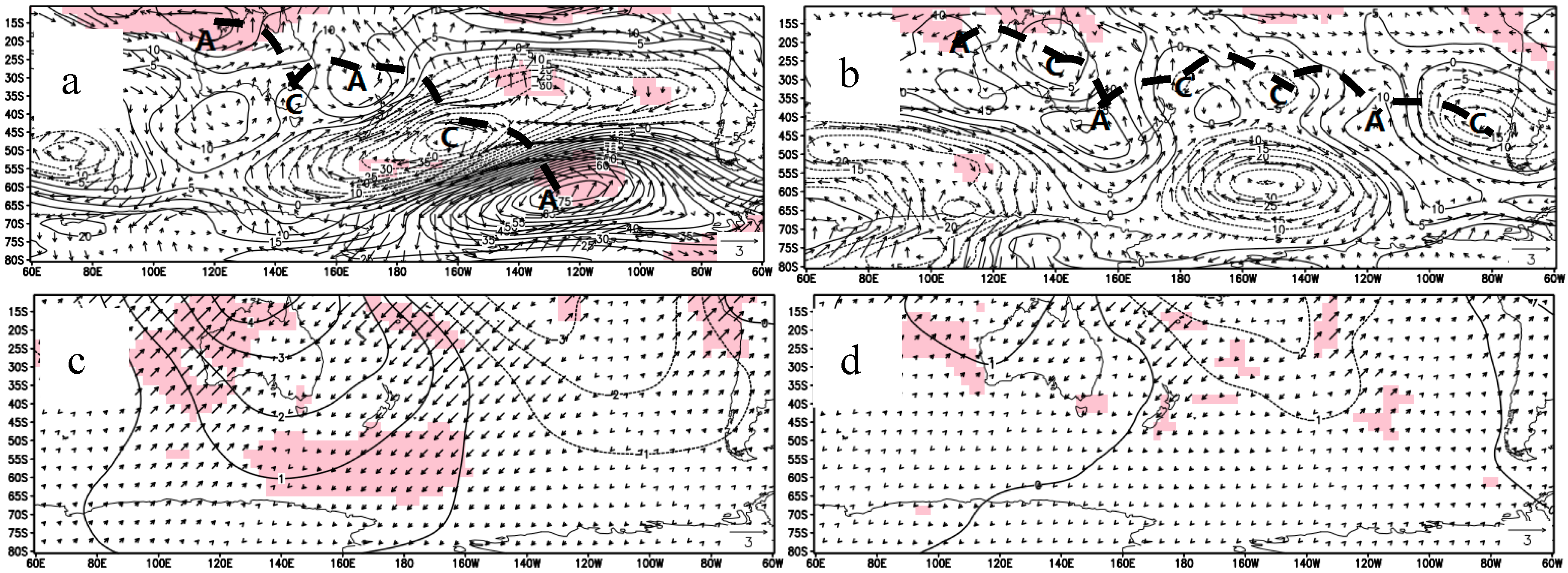
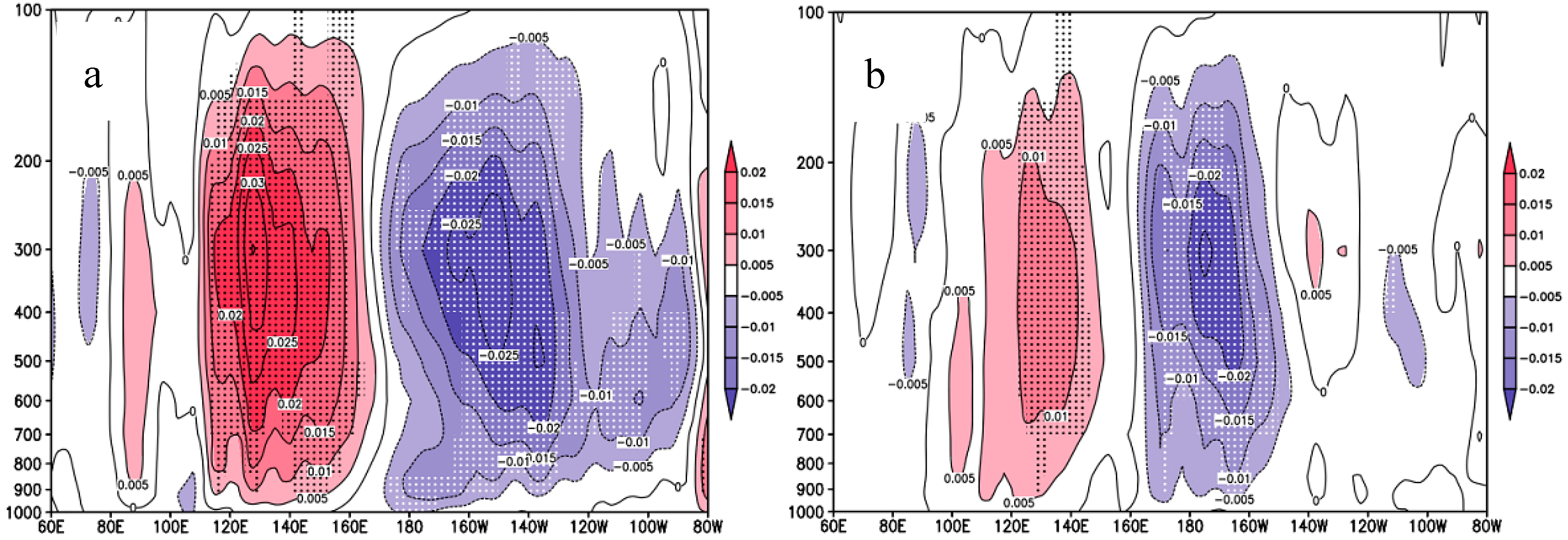
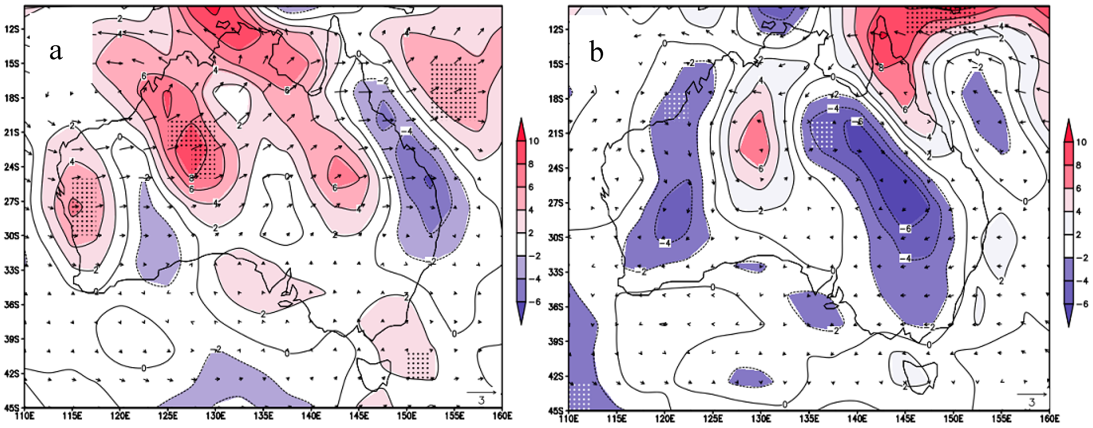
3.2.2. Composite Analysis for the Atmospheric Circulation Variability

Analyzing the southern hemisphere’s atmospheric variations associated with the Pacific SST anomalies, Figure 5a,b shows the anomalous horizontal winds at 700 hPa (cyclone and anticyclone indicated by “C” and “A”, respectively) and geopotential height at 500 hPa, while Figure 5c,d shows the anomalous velocity potential and divergent wind at 200 hPa. In the autumn El Niño mature phase of ENSO (DJF), at 700 hPa (Figure 5a), there were three anomalous anticyclones in the southern hemisphere: One over the wide area of the western Pacific [46], one centered 160° E (east of Australia), and the third one over the Ross Sea region. Meanwhile, there were two anomalous cyclones, one northeastern extended from the east of New Zealand to 130° W, and another over southeastern Australia. The northeastern coast of Australia was affected by anomalous westerly winds along the southern flank of the anomalous anticyclone and the northern flank of the anomalous cyclone. The westerly was not conducive to the transport of water vapor from the ocean to southeastern Australia. In addition, at 500 hPa a wave train was found in the middle and high latitudes of the southern hemisphere, with positive and negative anomalies alternately extending from the low latitudes toward the southeastern Pacific, that is, the Pacific South American (PSA) teleconnection [46]. Offshore flows prevailed in southeastern Australia, with air transported from inland to the sea. At 200 hPa, anomalous convergence of divergent wind was seen over the whole area of the western Pacific, including Australia (Figure 5c). This circulation was not conducive to rainfall in this area.
In the winter El Niño mature phase of ENSO (DJF), at 700 hPa (Figure 5b), there were three anomalous anticyclones: One over the tropical East Indian Ocean [47], one over the eastern coast of Australia, and the third one located within 130–100° W and 30–50° S. Meanwhile, there were three anomalous cyclones, one over central Australia, one over the east of New Zealand, and the third one centered 90° W (west of South America). Subtropical southeastern Australia was affected by anomalous northerly winds along the western flank of the anomalous anticyclone. The anomalous northerly transported water vapor from the ocean to southeastern Australia [37]. In addition (Figure 5b), at 500 hPa, the active centers of the PSA wave train shifted westward 20° and were weaker when compared to a normal year, for example, the geopotential height anomaly that was situated northeast of New Zealand decreased from −20 to −5 gpm. A 700-hpa large-scale pattern of cyclone/anticyclone anomalies that were more pronounced over the latitudes of Australia were stronger. Onshore flows prevailed in the northeastern coast of Australia while air flowed around the anticyclone off the east coast of Australia, where it picked up moisture from the marine, the air parcel moved inland, and was advected south into southeastern Australia. An anomalous 200-hPa divergence zone of divergent wind centered over the central tropical Pacific (Figure 5d) and anomalous convergence over Australia weakened when compared to autumn El Niño events. This circulation favored rainfall in this area.
In the autumn El Niño events, a 200-hPa anomalous convergence (Figure 5c), a 500-hPa larger positive geopotential height anomaly, and a 700-hPa anomalous westerly (Figure 5a) were not conducive factors to the formation of rainfall in southeastern Australian. In the winter El Niño episodes, a 200-hPa smaller convergence anomaly (Figure 5d), a 500-hPa smaller positive geopotential height anomaly, and a 700-hPa anomalous northerly (Figure 5b) were favorable factors for the formation of rainfall in this region, as the maritime air masses always contain more moisture than the continental ones and the northerly can result in a southward moisture transport to southeastern Australia, increasing the moisture supply there.
Dynamical consistency between the lower-level and upper-level anomalies is clear over southeastern Australia and the equatorial Pacific. From another view, the regional meridional and zonal circulation changes are also important factors contributing to the lower-to-upper level connection. The Walker circulation is the dominant zonal circulation over the near-equatorial South Pacific. In the austral autumn El Niño events (Figure 6a), the above-pronounced positive SST anomalies in the EEP generated a surface pressure lower than normal, while a wide-area anomalous ascending branch covered the entire eastern-central Pacific. Negative SST anomalies in the western equatorial Pacific (WEP) created a surface pressure higher than normal and a stronger, wider anomalous descent over the WEP (110–160° E). The Walker circulation was weakened, as depicted in Figure 6a. The descent regions encompassing the EEP ascent also formed a descent covering much of the extratropical South Pacific [48], adjusting local meridional cells, and, in turn, induced a descending anomaly over 15–38° S (Figure 7a), which was not the case in winter El Niño events (Figure 7b). In the winter El Niño events (Figure 6b), the CEP positive SST anomalies produced a double-cell anomalous pattern. The updraft near the date line and downdraft over the WEP (110–140° E) were weaker, with more of a westward shift than their counterparts in normal years. No obvious vertical motion anomalies were observed within 170° E–170° W. The adjustment of local meridional cells (170° E–170° W) was weaker too, resulting in a smaller descending anomaly over 15–30° S (Figure 7b), while updraft anomalies covered 32–38° S (zonal range of southeastern Australia). The result was consistent with the 700-hPa anomalous cyclone (Figure 5b, was stronger when compared to that of a normal year) over the region of 170° E–170° W and 32–38° S, enhancing the low-level troposphere convection there.
Thus, during autumn El Niño events, through the meridional, zonal circulations and anomalous wave train pattern, the signal of the EEP SST anomaly was transported to southeastern Australia and, consequently, the convective activity there was likely to be suppressed. In the winter El Niño events, when the anomalous wave train triggered by an anomalous cyclone (over 170° E–170° W and 30–40° S), traveled to southeastern Australia, it helped to develop convection there.
OLR is treated as a proxy for rainfall caused by convection. The anomalies of OLR were examined to demonstrate the convective activity difference between two flavors of El Niño events. During austral autumn El Niño events, negative OLR anomalies (Figure 8a) were collocated with negative rainfall anomalies over subtropical southeastern Australia (Figure 8c). Negative OLR anomalies (Figure 8b) in the winter El Niño events are associated with prosperity of convection and positive rainfall anomalies over there (Figure 8d). However, the use of OLR values at all atmospheric heights, as shown in Figure 8, may not provide the best representation of convection and rainfall anomalies in this area. This may suggest that the absence of a summer rainfall above normal over southeastern Australia during autumn El Niño events was related to non-precipitation high clouds with low OLR (e.g., cirrus) or a drier atmosphere, rather than precipitation clouds with low OLR (e.g., cumulonimbi) or moist atmosphere [49]. Therefore, we examined the water vapor transport as described below.

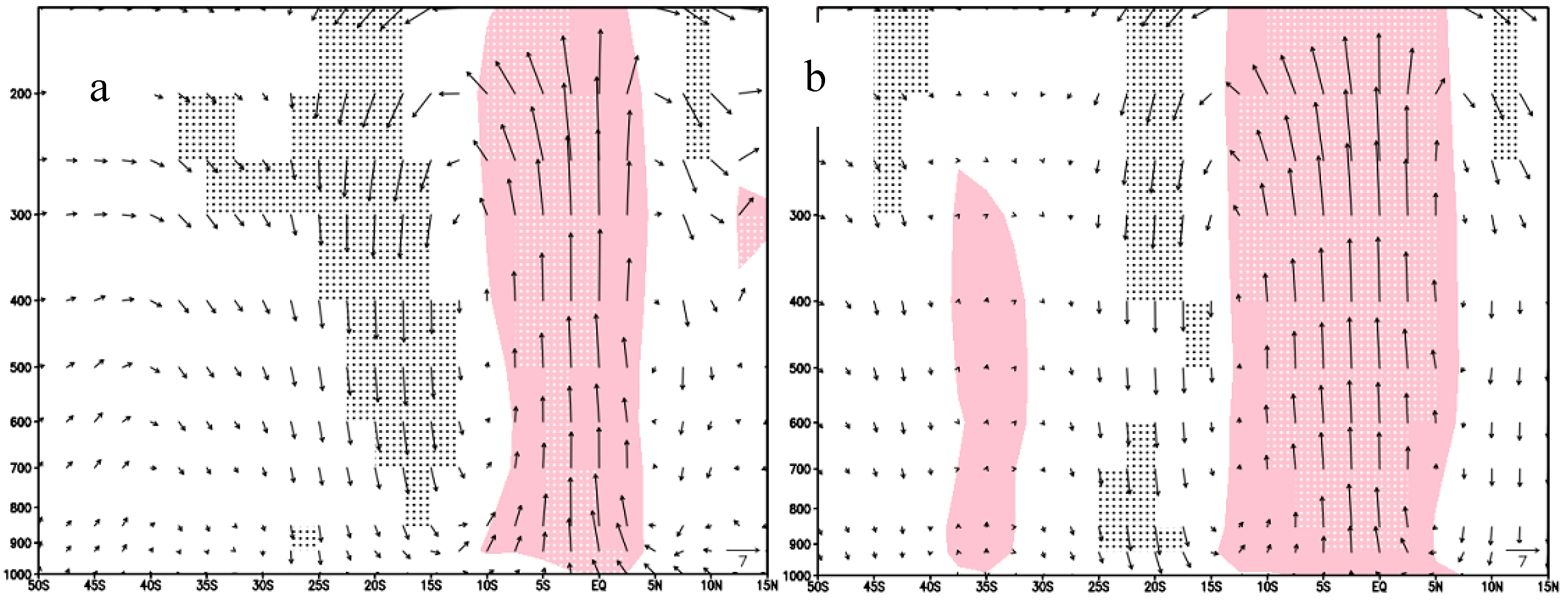
3.3. Composite Analysis for Water Vapor Transport

Figure 9 shows water vapor flux in the composites of autumn and winter El Niño events during DJF 1980–2017, separately. There was an anomalous water vapor sink anomaly at 850 hPa over southeastern Australia (Figure 9b), though not covering the whole region, during the winter El Niño events. During the autumn El Niño events, this area was almost covered by an anomalous water vapor divergence (Figure 9a). During winter El Niño events, the atmosphere was relatively more humid (Figure 9b), with a low-level troposphere anomalous ascent (Figure 7b), which favored rainfall over this region. In contrast, the low-level moisture divergence over the same area during autumn El Niño events, with an anomalous descent (Figure 7a), provided a below normal summer rainfall.

4. Discussion

It can be argued that the summer rainfall maybe actually be related to the intensity of the DJF Niño 3.4 index. We suggest with caution that the start time is a useful metric for seasonal prediction, because it tells the future strength and impacts on SASR, two to three seasons prior to the mature phase of El Niño.

5. Conclusions

The purpose of this work is to investigate and understand the different impacts of two types of El Niño events on summer rainfall over southeastern Australia. Their relationships featured obvious differences according to the onset time of El Niño events. Our work demonstrates that:
Summer rainfall over southeastern Australia tended to be lower than normal in austral autumn El Niño events and higher than normal in austral winter El Niño events, during DJF 1980–2017.
During autumn El Niño events, the Walker circulation and meridional cells served as a bridge linking the warmer SST in the EEP and lower SASR. This physical process can be described as follows: During DJF, a positive SST anomaly in the EEP was concurrent with anomalous downdraft over southeastern Australia via zonal anomalous Walker circulation along the equatorial Pacific, meridional anomalous cells along 170° E–170° W, and a PSA teleconnection wave train at 500 hPa. In addition, an anomalous convergence at 200 hPa depressed the convection. Meanwhile, an 850-hPa abnormal westerly was not conducive to transport marine water vapor into this area. These factors resulted in below-normal rainfall over this region. During winter El Niño events, a positive SST anomaly in the CEP and the change in the Walker circulation and meridional cells were weaker. The PSA teleconnection wave train shifted westward and northward, and there was a low-level anomalous ascent over southeastern Australia. At the western flank of the anomalous anticyclone, northerly transported water vapor from the ocean to southeastern Australia resulted in a sink of water vapor over this area (non-significant). The development of low-level convective activity and the plentiful water vapor supply favored more rainfall over southeastern Australia.

Author Contributions

Conceptualization, L.F. and J.X.; Methodology, L.F.; Software, L.F.; Validation, L.F., J.X. and L.H.; Formal Analysis, L.F.; Investigation, L.F.; Resources, L.F.; Data Curation, L.F.; Writing—Original Draft Preparation, L.F.; Writing—Review & Editing, L.F.; Visualization, L.F.; Supervision, J.X.; Project Administration, L.F. and L.H.; Funding Acquisition, J.X.

Funding

This study was funded by National Key Research and Development Program of China with No 2018YFC1506002.

Acknowledgments

The authors wish to thank the anonymous reviewers for their constructive comments.

Conflicts of Interest

The authors declare no conflict of interest.

References

  1. Kane, R.P. On the relationship of ENSO with rainfall over different parts of Australia. Aust. Meteorol. Mag. 1996, 46, 39–49. [Google Scholar]
  2. Murphy, B.F.; Timbal, B. A review of recent climate variability and climate change in southeastern Australia. Int. J. Climatol. 2008, 28, 859–879. [Google Scholar] [CrossRef] [Green Version]
  3. Pezza, A.B.; Burrant, T.; Simmonds, I.; Smith, I. Southern Hemisphere Synoptic Behavior in Extreme Phases of SAM, ENSO, Sea Ice Extent, and Southern Australia Rainfall. J. Clim. 2010, 21, 5566–5584. [Google Scholar] [CrossRef]
  4. Sturman, A.P.; Tapper, N.J. The Weather and Climate of Australia and New Zealand; Oxford University Press: Oxford, UK, 2006; Volume 438. [Google Scholar]
  5. Croke, J.; Reinfelds, I.; Thompson, C.; Roper, E. Macrochannels and their significance for flood-risk minimisation: Examples from southeast Queensland and New South Wales, Australia. Stoch. Environ. Res. Risk Assess. 2014, 28, 99–112. [Google Scholar] [CrossRef]
  6. Hendon, H.H.; Lim, E.P.; Arblaster, J.M.; Anderson, D.L.T. Causes and predictability of the record wet east Australian spring 2010. Clim. Dyn. 2014, 42, 1155–1174. [Google Scholar] [CrossRef]
  7. Lim, E.P.; Hendon, H.H. Understanding and predicting the strong Southern Annular Mode and its impact on the record wet east Australian spring 2010. Clim. Dyn. 2015, 44, 2807–2824. [Google Scholar] [CrossRef]
  8. Mcbride, J.L.; Nicholls, N. Seasonal relationships between Australian rainfall and the southern oscillation. Mon. Weather Rev. 1983, 111, 1998–2004. [Google Scholar] [CrossRef]
  9. Karoly, D.J. Southern Hemisphere circulation features associated with El Niño–Southern Oscillation events. J. Clim. 1989, 2, 1239–1252. [Google Scholar] [CrossRef]
  10. Power, S.; Casey, T.; Folland, C.; Colman, A.; Mehta, V. Inter-decadal modulation of the impact of ENSO on Australia. Clim. Dyn. 1999, 15, 319–324. [Google Scholar] [CrossRef]
  11. Harangozo, S. A search for ENSO teleconnections in the west Antarctic Peninsula climate in austral winter. Int. J. Climatol. 2000, 20, 663–679. [Google Scholar] [CrossRef] [Green Version]
  12. Wang, G.; Hendon, H.H. Sensitivity of Australian rainfall to inter–El Nino variations. J. Clim. 2007, 20, 4211–4226. [Google Scholar] [CrossRef]
  13. Ashok, K.; Guan, Z.; Yamagata, T. Influence of the Indian Ocean Dipole on the Australian winter rainfall. Geophys. Res. Lett. 2003, 30, 1329. [Google Scholar] [CrossRef]
  14. Acworth, R.I.; Rau, G.C.; Cuthbert, M.O.; Jensen, E.; Leggett, K. Long-term spatio-temporal precipitation variability in arid-zone Australia and implications for groundwater recharge. Hydrogeol. J. 2016, 24, 1–17. [Google Scholar] [CrossRef]
  15. Cai, W.J.; Van Rensch, P.; Cowan, T.; Hendon, H.H. An asymmetry in the IOD and ENSO teleconnection pathway and its impact on Australian climate. J. Clim. 2011, 25, 6318–6329. [Google Scholar] [CrossRef]
  16. Ihara, C.; Kushnir, Y.; Cane, M.A.; De La Pena, V.H. Indian summer monsoon rainfall and its link with ENSO and Indian Ocean climate indices. Int. J. Climatol. 2007, 27, 179–187. [Google Scholar] [CrossRef] [Green Version]
  17. Meyers, G.; McIntosh, P.; Pigot, L.; Pook, M. The years of El Nino, La Nina, and interactions with the tropical Indian Ocean. J. Clim. 2007, 20, 2872–2880. [Google Scholar] [CrossRef]
  18. Verdon, D.C.; Franks, S.W. Long-term behaviour of ENSO: Interactions with the PDO over the past 400 years inferred from paleoclimate records. Geophys. Res. Lett. 2006, 33, 272–288. [Google Scholar] [CrossRef]
  19. Meneghini, B.; Simmonds, I.; Smith, I.N. Association between Australian rainfall and the southern annular mode. Int. J. Climatol. 2007, 27, 109–121. [Google Scholar] [CrossRef]
  20. Hendon, H.H.; Thompson, D.W.J.; Wheeler, M.C. Australian rainfall and surface temperature variations associated with the southern hemisphere annular mode. J. Clim. 2007, 20, 2452–2467. [Google Scholar] [CrossRef]
  21. Lim, E.P.; Hendon, H.H.; Arblaster, J.M.; Delage, F.; Nguyen, H.; Min, S.K.; Wheeler, M.C. The impact of the southern annular mode on future changes in southern hemisphere rainfall. Geophys. Res. Lett. 2016, 43, 7160–7167. [Google Scholar] [CrossRef]
  22. Thompson, D.W.J.; Wallace, J.M. Annular modes in the extratropical circulation. part I: Month-to-month variability. J. Clim. 2000, 13, 1000–1016. [Google Scholar] [CrossRef]
  23. Xie, Z.Y.; Huete, A.; Restrepo-Coupe, N.; Ma, X.L.; Devadas, R.; Caprarelli, G. Spatial partitioning and temporal evolution of Australia’s total water storage under extreme hydroclimatic impacts. Remote Sens. Environ. 2016, 183, 43–52. [Google Scholar] [CrossRef]
  24. Ropelewski, C.F.; Halpert, M.S. Global and regional scale precipitation patterns associated with the El Niño/Southern Oscillation. Mon. Weather Rev. 1987, 115, 1606–1626. [Google Scholar] [CrossRef]
  25. McPhaden, M.J.; Zebiak, S.E.; Glantz, M.H. ENSO as an integrating concept in earth science. Science 2006, 314, 1740–1745. [Google Scholar] [CrossRef] [PubMed]
  26. Gallant, A.J.E.; Kiem, A.S.; Verdon-Kidd, D.C.; Stone, R.C.; Karoly, D.J. Understanding hydroclimate processes in the Murray-Darling Basin for natural resources management. Hydrol. Earth Syst. Sci. 2012, 16, 2049–2068. [Google Scholar] [CrossRef] [Green Version]
  27. Taschetto, A.S.; England, M.H. El Niño Modoki impacts on Australian rainfall. J. Clim. 2009, 22, 3167–3174. [Google Scholar] [CrossRef]
  28. Zhu, Z.W. Breakdown of the Relationship between Australian Summer Rainfall and ENSO Caused by Tropical Indian Ocean SST Warming. J. Clim. 2018, 31, 2321–2336. [Google Scholar] [CrossRef]
  29. Hendon, H.H.; Lim, E.-P.; Liu, G. The role of air–sea interaction for prediction of Australian summer monsoon rainfall. J. Clim. 2012, 25, 1278–1290. [Google Scholar] [CrossRef]
  30. Yasunari, T. Zonally propagating modes of the global east-west circulation associated with the Southern Oscillation. J. Meteorol. Soc. Jpn. 1985, 63, 1013–1029. [Google Scholar] [CrossRef]
  31. Fu, C.B.; Diaz, H.F.; Fletcher, J.O. Characteristics of the response of sea surface temperature in the central Pacific associated with warm episodes of the Southern Oscillation. Mon. Weather Rev. 1986, 114, 1716–1738. [Google Scholar] [CrossRef]
  32. Quinn, W.H.; Neal, V.T. El Niño occurrences over the past four and a half centuries. J. Geophys. Res. 1987, 92, 14449–14461. [Google Scholar] [CrossRef]
  33. Enfield, D.B.; Cid, L.S. Low-frequency changes in El Niño–Southern Oscillation. J. Clim. 1991, 4, 1137–1146. [Google Scholar] [CrossRef]
  34. Wang, S. Reconstruction of El Niño event chronology for the last 600-year period. Acta Meteorol. Sin. 1992, 6, 47–57. (In Chinese) [Google Scholar]
  35. Xu, J.J.; Chan, J.C.L. The role of the Asian-Australian monsoon system in the onset time of El Niño events. J. Clim. 2001, 14, 418–433. [Google Scholar] [CrossRef]
  36. Timmermann, A.; An, S.I.; Kug, J.S.; Jin, F.F.; Cai, W.J.; Capotondi, A.; Cobb, K.; Lengaigne, M.; McPhaden, M.J.; Stuecker, M.F.; et al. El Niño–Southern Oscillation complexity. Nature 2018, 559, 535–545. [Google Scholar] [CrossRef]
  37. Brown, J.N.; Mcintosh, P.C.; Pook, M.J.; Risbey, J.S. An Investigation of the Links between ENSO Flavors and Rainfall Processes in Southeastern Australia. Mon. Weather Rev. 2009, 137, 3786–3795. [Google Scholar] [CrossRef]
  38. Hirahara, S.; Ishii, M.; Fukuda, Y. Centennial-scale sea surface temperature analysis and its uncertainty. J. Clim. 2014, 27, 57–75. [Google Scholar] [CrossRef]
  39. Kalnay, E.; Kanamitsu, M.; Kistler, R.; Collins, W.; Deaven, D.; Gandin, L.; Iredell, M.; Saha, S.; White, G.; Woollen, J.; et al. The NCEP/NCAR 40-year reanalysis project. Bull. Am. Meteorol. Soc. 1996, 77, 437–470. [Google Scholar] [CrossRef]
  40. Lee, H.T.; Gruber, A.; Ellingson, R.G.; Laszlo, I. Development of the HIRS Outgoing Longwave Radiation climate data set. J. Atmos. Ocean. Technol. 2007, 24, 2029–2047. [Google Scholar] [CrossRef]
  41. Fan, L.L.; Xu, J.J.; Guan, H.D. Impacts of Different Onset Time El Niño Events on Winter Rainfall over South China. Atmosphere 2018, 9, 366. [Google Scholar] [CrossRef]
  42. Sun, J.Q.; Wang, H.J.; Yuan, W. A possible mechanism for the co-variability of the boreal spring Antarctic Oscillation and the Yangtze River valley summer rainfall. Int. J. Climatol. 2009, 29, 1276–1284. [Google Scholar] [CrossRef] [Green Version]
  43. Lim, E.P.; Hendon, H.H. Causes and Predictability of the Negative Indian Ocean Dipole and Its Impact on La Nina During 2016. Sci. Rep. 2017, 7, 12619. [Google Scholar] [CrossRef] [PubMed]
  44. Michael, A.B.; Gail, P. Physics of Radiation and Climate; CRC Press: Boca Raton, FL, USA, 2015; p. 151. [Google Scholar]
  45. Risbey, J.S.; Pook, M.J.; McIntosh, P.C.; Wheeler, M.C.; Hendon, H.H. On the remote drivers of rainfall variability in Australia. Mon. Weather Rev. 2009, 137, 3233–3253. [Google Scholar] [CrossRef]
  46. Mo, K.C.; Higgins, R.W. The Pacific-South American modes and tropical convection during the Southern Hemisphere winter. Mon. Weather Rev. 1998, 126, 1581–1596. [Google Scholar] [CrossRef]
  47. Yeo, S.R.; Kim, K.Y. Decadal changes in the Southern Hemisphere sea surface temperature in association with El Niño–Southern Oscillation and Southern Annular Mode. Clim. Dyn. 2015, 45, 3227–3242. [Google Scholar] [CrossRef] [Green Version]
  48. Weng, H.; Behera, S.K.; Yamagata, T. Anomalous winter climate conditions in the Pacific rim during recent El Niño Modoki and El Niño events. Clim. Dyn. 2009, 32, 663–674. [Google Scholar] [CrossRef]
  49. Rauniyar, S.P.; Walsh, K.J.E. Influence of ENSO on the Diurnal Cycle of Rainfall over the Maritime Continent and Australia. J. Clim. 2013, 26, 1304–1321. [Google Scholar] [CrossRef]
Figure 1. Composite time series of SST anomalies in the Niño 3.4 region (unit: °C) for austral autumn (open circles) and winter (solid circles) El Niño events during 1956–2017.
Atmosphere 10 00139 g001
Figure 2. Averaged (a) austral summer rainfall (units: mm; contour interval: 100 mm) and (b) summer rainfall percentage (units: %; contour interval: 10%) during December–January–February (DJF) 1980–2017. The red rectangle denotes the location of southeastern Australia (25–44° S, 136–155° E).
Atmosphere 10 00139 g002
Figure 3. Temporal evolution of the Niño 3.4 SST anomaly (blue; units: °C) and normalized austral summer rainfall (orange) over southeastern Australia in DJF 1980–2017.
Atmosphere 10 00139 g003
Figure 4. Composite SST anomalies (units: °C) during DJF 1980–2017 for (a) autumn and (b) winter El Niño events. The contour interval is 0.3 °C. Only values significant at the 95% level have been shaded, based on the Student’s t-test.
Atmosphere 10 00139 g004
Figure 5. Composites of anomalies of (a) 700-hPa horizontal wind (units: m·s−1) and 500-hPa geopotential height (contours; units: gpm; the contour interval is 5 gpm) and (c) 200-hPa velocity potential (contours; units: 106 m2·s−1; the contour interval is 1 × 10⁶ m2·s−1); divergent wind (vector; units: m·s−1) during DJF 1980–2017 for austral autumn El Niño events. Panels (b) and (d) show the same but for winter El Niño events. The wind scale is shown at the bottom of the respective panels. Shaded areas indicate statistical significance at the 95% confidence level, based on the Student’s t-test.
Atmosphere 10 00139 g005
Figure 6. Composite anomalies of longitude–pressure cross-sections of vertical velocity (units: hPa·s−1) averaged along 15° S–15° N during DJF 1980–2017 for (a) austral autumn and (b) winter El Niño events. Dotted areas indicate statistically significant vertical velocity at the 95% confidence level, based on the Student’s t-test.
Atmosphere 10 00139 g006
Figure 7. Composite anomalies of latitude–pressure cross-sections of meridional circulations (vectors) averaged along 170° E–170° W during DJF 1980–2017 for austral autumn (a) and winter (b) El Niño events. The units for meridional wind and vertical motion are m·s−1 and hPa·s−1, respectively. The values of vertical velocity are multiplied by −300. Shaded areas have an upward vertical velocity of ≥0.01 hPa·s−1. Dotted areas indicate statistically significant vertical velocity at the 95% confidence level, based on the Student’s t-test.
Atmosphere 10 00139 g007
Figure 8. Composite outgoing longwave radiation (OLR) (units: W·m−2) anomalies during DJF 1980–2017 for the austral (a) autumn and (b) winter El Niño events, the contour interval is 3 W·m−2. Shaded areas are statistically significant at the 95% confidence level, based on the Student’s t-test. (c) and (d) are the same as (a) and (b), but for summer rainfall anomalies, the contour interval is 30 mm.
Atmosphere 10 00139 g008
Figure 9. Composite water vapor flux anomaly at 850 hPa (vectors; units: g·cm−1·hPa−1·s−1) and its divergence (contours; units: 10−7g·cm−2·hPa−1·s−1) in the austral (a) autumn and (b) winter El Niño events. Dotted areas indicate statistical significance at the 95% confidence level, based on the Student’s t-test.
Atmosphere 10 00139 g009
Table 1. Classification of El Niño events during 1980–2017.
SequenceDurationLength (in Months)Onset_TimeType
1May 1982–June 198314AprilAU
2August 1986–January 198818JulyWI
3June 1991–June 199213MayAU
4September 1994–February 19956AugustWI
5May 1997–May 199813AprilAU
6June 2002–February 20039MayAU
7July 2004–March 20059JuneWI
8July 2009–March 20109JuneWI
9April 2015–April 201613MarchAU

