Major Source Contributions to Ambient PM_2.5 and Exposures within the New South Wales Greater Metropolitan Region

Abstract

The coupled Conformal Cubic Atmospheric Model (CCAM) and Chemical Transport Model (CTM) (CCAM-CTM) was undertaken with eleven emission scenarios segregated from the 2008 New South Wales Greater Metropolitan Region (NSW GMR) Air Emission Inventory to predict major source contributions to ambient PM_2.5 and exposure in the NSW GMR. Model results illustrate that populated areas in the NSW GMR are characterised with annual average PM_2.5 of 6–7 µg/m³, while natural sources including biogenic emissions, sea salt and wind-blown dust contribute 2–4 µg/m³ to it. Summer and winter regional average PM_2.5 ranges from 5.2–6.1 µg/m³ and 3.7–7.7 µg/m³ across Sydney East, Sydney Northwest, Sydney Southwest, Illawarra and Newcastle regions. Secondary inorganic aerosols (particulate nitrate, sulphate and ammonium) and sodium account for up to 23% and 18% of total PM_2.5 mass in both summer and winter. The increase in elemental carbon (EC) mass from summer to winter is found across all regions but particularly remarkable in the Sydney East region. Among human-made sources, “wood heaters” is the first or second major source contributing to total PM_2.5 and EC mass across Sydney in winter. “On-road mobile vehicles” is the top contributor to EC mass across regions, and it also has significant contributions to total PM_2.5 mass, particulate nitrate and sulphate mass in the Sydney East region. “Power stations” is identified to be the third major contributor to the summer total PM_2.5 mass across regions, and the first or second contributor to sulphate and ammonium mass in both summer and winter. “Non-road diesel and marine” plays a relatively important role in EC mass across regions except Illawarra. “Industry” is identified to be the first or second major contributor to sulphate and ammonium mass, and the second or third major contributor to total PM_2.5 mass across regions. By multiplying modelled predictions with Australian Bureau of Statistics 1-km resolution gridded population data, the natural and human-made sources are found to contribute 60% (3.55 µg/m³) and 40% (2.41 µg/m³) to the population-weighted annual average PM_2.5 (5.96 µg/m³). Major source groups “wood heaters”, “industry”, “on-road motor vehicles”, “power stations” and “non-road diesel and marine” accounts for 31%, 26%, 19%, 17% and 6% of the total human-made sources contribution, respectively. The results in this study enhance the quantitative understanding of major source contributions to ambient PM_2.5 and its major chemical components. A greater understanding of the contribution of the major sources to PM_2.5 exposures is the basis for air quality management interventions aiming to deliver improved public health outcomes.

1. Introduction

Exposure to ambient PM_2.5 has well-documented associations with increased risk of mortality [1], lower life expectancy [2] and a range of health effects, such as respiratory diseases [3], cardiovascular diseases [4] and low birth weight [5]. Even through air quality in New South Wales Greater Metropolitan Region (NSW GMR) is generally classified as good when compared to national air quality standards [6], PM_2.5 air pollution continues to have a significant impact on human health and the economy [7]. Health effects occur even at exposure levels below national air quality standards as there is no evidence of a safe level of exposure to PM_2.5 [8]

Particulate matter is an important atmospheric pollutant that can be directly emitted into the atmosphere (primary PM) or produced via chemical reactions of precursors (secondary PM). Human activities such as motor vehicles, residential wood heaters, mining, industry, power generation and non-road vehicles and equipment contribute to particle pollution (e.g., [9,10]). Exceedances of national air quality standards due to high PM_2.5 concentrations are frequently associated with regional dust storms and vegetation fires [11].

To devise effective air pollution control strategies to reduce ambient PM_2.5 concentrations, it is necessary to understand how the emissions from a range of sources contribute to ambient concentrations. Particles can be made up of a range of chemical species depending on the source of the particle or the precursor gases from which they form. The methods used to investigate the contribution from different sources to PM_2.5 are generally referred as source apportionment methods and their results are considered to be crucial to inform air quality management planning [12]. Three commonly used source apportionment methods are as summarised in

Table 1. Modelling scenarios for the 2008 calendar year.

Modelling Scenarios			Emission Sources Groups
1.Base case	2. Human-made sources	4. Power stations	Power generation from coal
			Power generation from gas
		5. Wood heaters	Residential wood heaters
		6. On-road motor vehicles	Petrol exhaust
			Diesel exhaust
			Other exhaust
			Petrol evaporation
			Non-exhaust particulate matter
		7. Non-road diesel and marine	Shipping and commercial boats
			Industrial vehicles and equipment
			Aircraft (flight and ground operations)
			Locomotives
			Commercial non-road equipment
		8. Industry	Other industrial point sources (all point source emissions except power generation from coal and gas)
		9. Human-made other	Emissions from anthropogenic sources other than listed above, e.g., other commercial and domestic-commercial area source emissions, and industrial area fugitive emissions
	3. Natural sources	10. Biogenic	Biogenic sources
		11. Natural other	Emissions from regional wind-blown dust and sea salt

of [13]. The receptor-based mathematical tools, also known as ‘receptor models’, are observation-based and often used to estimate source contributions to particle concentrations at the measurement sites. Positive matrix factorisation (PMF) is a widely applied receptor modelling technique recently used in regional air quality studies in NSW, Australia ([9,14,15]). The Upper Hunter Valley Particle Characterization Study [14] investigated the composition and sources of PM_2.5 in Singleton and Muswellbrook, the major population centres in the Upper Hunter region, to address community concerns about PM_2.5 pollution from the open-cut coal mines and the coal-fired power stations. The study identified residential wood smoke to be a significant component of fine particle concentrations in winter, with secondary sulphate and industry aged salt contributing to concentrations in the summer. The Lower Hunter Particle Characterisation Study [9] investigated the composition and major sources of PM_2.5 pollution in the Lower Hunter region and sources of PM₁₀ in the vicinity of the Port of Newcastle. Measurements were conducted at Newcastle and Beresfield to characterised regional population exposures and at two sites (Mayfield and Stockton) near the Port of Newcastle. Nine source groups were identified as contributing to fine particles, namely, fresh sea salt, pollutant-aged sea salt, secondary ammonium sulphate, soil, wood smoke, vehicles, mixed shipping and industry, mixed industry and vehicles and nitrate. Based on fifteen years of sampling data at four sites across Greater Sydney (Lucas Heights, Richmond, Mascot and Liverpool), the Sydney Particle Characterisation Study used the PMF source apportionment technique to identify and quantify the sources of fine particle pollution [15]. Sydney’s air was found to be characterised by fine particles from wood smoke, industry, vehicles, sea salt and soil; smoke (including from residential wood burning) contributed 60% to 80% of fine particles at some sites in the winter months and secondary sulphates (emissions from coal-fired power stations and industry) contributed 50% to 70% of fine particles in summer at some sites. Particles from automobiles declined by 40% over the 15 years, but motor vehicles were found to remain a significant source of fine particle pollution in Greater Sydney.

Regional airshed modelling is another powerful and widely applied tool for source apportionment. It is a source-based (emission-based) method opposed to a receptor-based method and may provide more detailed composition information and greater spatial and temporal resolution of air pollution impacts. The most straightforward method is to conduct emission source sensitivity simulations by turning off (or reducing) emissions from specific source (e.g., [16]); the source contributions to air pollutants can be approximately estimated between the results from the sensitivity and baseline simulations. This brute force method (BFM) or zero-out method has been widely used in source sensitivity studies of major pollutants worldwide (e.g., [13] and [17] ). While it is a popular tool for policy-maker to analyse the effects of emissions reduction on air quality, the non-linear effects between changes in emissions of SO₂, NOx and VOC and changes in PM_2.5 mass and component (sulphate, nitrate, ammonium and organic compounds) concentrations is addressed [18]. And it is not always practical because computational cost increases linearly with the number of emissions scenarios to examine, and the smaller concentration changes between the simulations may be strongly influenced by numerical errors as noted in [19]. The efficiency and flexibility in this source-based method has been improved by applying the Particulate Source Apportionment Technology (PSAT). The tagged species in PSAT apportions concentrations of PM components to their respective primary precursors (e.g., sulphate is apportioned to SOx, nitrate to NOx, etc.) making it possible to run one single simulation and obtain various source contributions [20]. Source contributions estimated from BFM and PSAT generally agree well for primary pollutants but may produce significantly different results for secondary pollutants [13].

The Sydney Particle Study commissioned by the NSW Office of Environment and Heritage (NSW OEH) comprised field measurement campaigns and a program of chemical transport modelling development and application [21]. This combined monitoring-modelling study showed seasonally varying composition of fine particles and demonstrated the applicability of the coupled Conformal Cubic Atmospheric Model (CCAM) and a Chemical Transport Model (CTM) (hereafter, the CCAM-CTM). The CCAM-CTM modelling system had also been selected by NSW OEH to support regional modelling of ozone, primary and secondary particles and other air pollutants in NSW to inform air policies and programs and provide information to communities [22,23].

Accurately assessing source contributions to population exposure to ambient air pollution supports the tailoring of air pollution management strategies to target sources contributing significantly to human health risk. Over the last decade, regional air quality models have matured and are being used for population air pollution exposure estimation and related health impact assessment (e.g., [24,25]). In this study, the CCAM-CTM modelling system was configured for regional meteorological and air quality modelling for the NSW GMR and run for the whole calendar year of 2008. The aims of this study are:

• to characterise spatio-temporal variations in PM_2.5 concentrations for the NSW GMR;
• to quantify major source contributions to PM_2.5 concentrations and the major chemical components of PM_2.5 (sulphate, nitrate, ammonium, elemental carbon and sodium) in the sub-regions across NSW GMR; and
• to quantify major source contributions to population-weighted annual average PM_2.5 concentrations to support source apportionment of the health burden associated with fine particle exposures in the NSW GMR.

2. Methodology

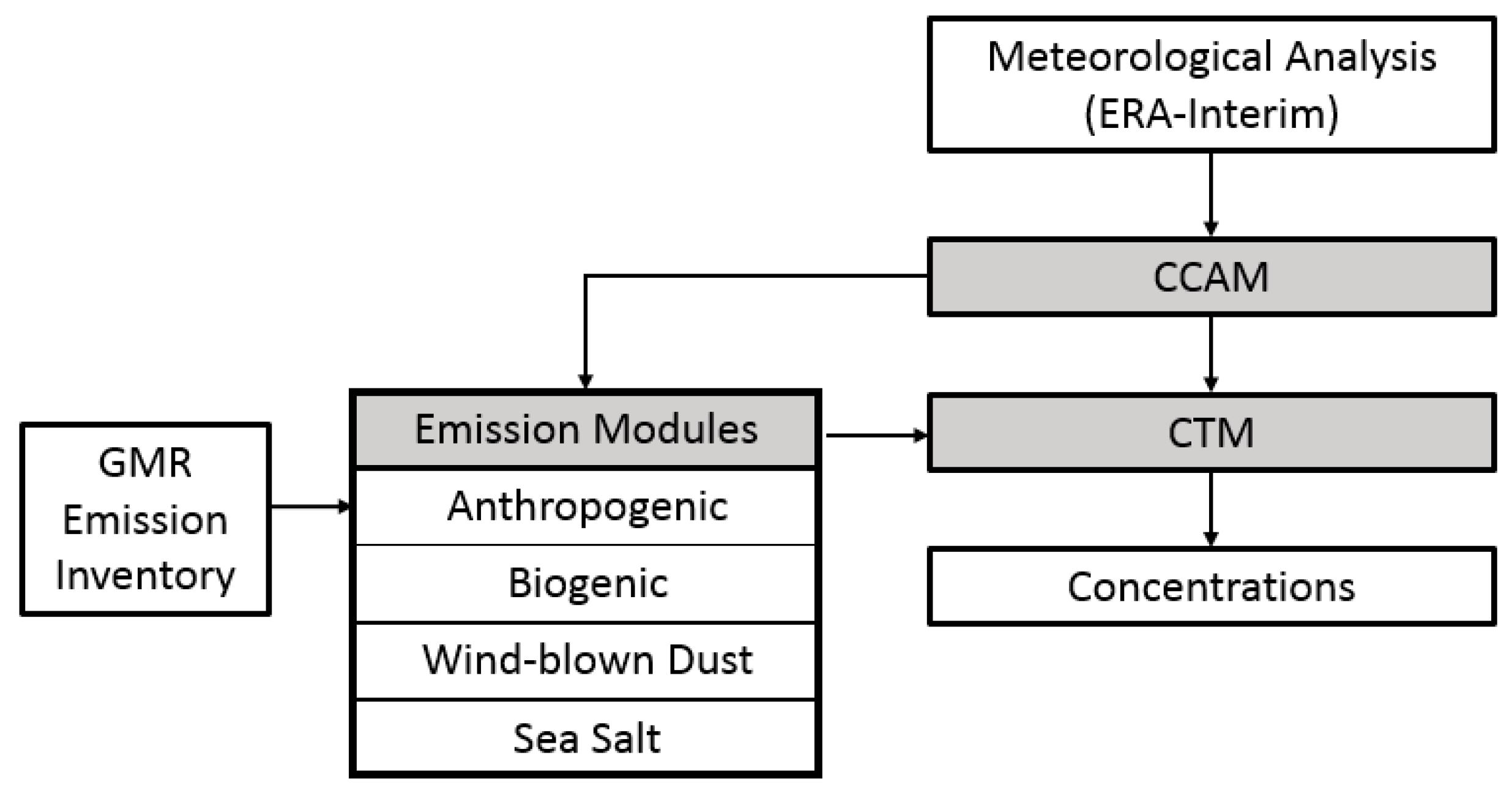
2.1. Modelling System Setup

The CCAM-CTM modelling system implemented in this study combines a meteorology module (CCAM) [26], emission module, and a chemical transport module (CTM) [27]. The schematic diagram of the modelling system is illustrated in Figure 1. CCAM-CTM modelling was undertaken using four nested domains, comprising the outermost Australian domain (CTM AUS) at 80-km × 80-km resolution (75 × 65 grid cells), the New South Wales (CTM NSW) domain at 27-km × 27-km (60 × 60 grid cells), the Greater Metropolitan Region (CTM GMR) at 9-km × 9-km resolution (60 × 60 grid cells) and the innermost domain covering Greater Sydney regional airshed (CTM GSYD) at 3-km × 3-km resolution (60 × 60 grid cells). The configurations for CTM GMR and CTM GSYD domains are shown in Figure 2.

In this study, the European Reanalysis Interim (ERA-Interim) reanalysis was the host general circulation model (GCM) data and was fed into CCAM and downscaled into four nested domains. A 35 vertical levels configuration of CCAM was applied. The model configurations of CCAM used in this study is summarized in

Table A1. CCAM configurations.

Model Specifications	Model Version	CCAM r3019 (Released May 2016)
Domain	Number of nests	4
	Horizontal resolution (for each nest)	80 km, 27 km, 9 km, 3 km
	Number of x grid points (per nest)	75, 60, 60, 60
	Number of y grid points (per nest)	65, 60, 60, 60
	Number of vertical layers	35
	Height of first layer	10 m
Initial & Boundary conditions	Meteorology input	ERA-Interim
	Analysis and initialization	CCAM use a scale-selective filter to assimilate (or nudge) CCAM towards the ERA-Interim data
Parameterisations	Microphysics scheme	Cloud microphysics with prognostic condensate (Rotstayn 1997)
	Longwave radiation scheme	Schwarzkopf and Ramaswamy (1991)
	Shortwave radiation scheme	Freidenreich and Ramaswamy (1999)
	Land surface scheme	CABLE land-surface (Kowalczyk et al. 2006)
	Planetary Boundary Layer/turbulence scheme	McGregor et al. (1993) and Holtslag and Boville (1993)
	Convection scheme	McGregor (2003)
	Aerosol scheme	Rotstayn and Lohmann (2002)
Planetary Boundary Layer Height (PBLH) calculations	Description	Equation 3.11 documented in Holtslag and Boville (1993) use a critical bulk Richardson number of 0.25 (not 0.5 as in the paper).

.

The CTM was then run with concentrations of gas and particulate-phase species model at the outermost boundary adapted from a global run of the United Kingdom Chemistry and Aerosol scheme (UKCA) for the UK Met Office Unified Model. The photochemical mechanisms for use in the current CTM is an extended version of the Carbon Bond 5 [28] with updated toluene chemistry [29]. An extended aerosol scheme was applied, where the secondary inorganic aerosols (SIA) were assumed to exist in thermodynamic equilibrium with gas phase precursors and were modelled using the ISORROPIA-II model [30] and the secondary organic aerosol (SOA) was modelled using the Volatility Basis Set approach [31] as documented in [21]. The model configurations of CTM used in this study is summarized in

Table A2. CTM configurations.

Model Version: CTM r1057 (Released August 2016)
Model Specifications
Domain	Number of nests	4
	Horizontal resolution (for each nest)	80 km, 27 km, 9 km, 3 km
	Number of x grid points (for each nest)	75, 60, 60, 60
	Number of y grid points (for each nest)	65, 60, 60, 60
	Number of vertical layers	16
	Height of first layer	20 m
Initial & Boundary conditions	Chemical BCs	UKCA (a mixture of UKCA for particles, and recommendations from Ian Galbally for VOCs and O3)
Emissions	Anthropogenic	2008 NSW GMR Air Emissions Inventory
	Biogenic	Calculated in-line with CTM
	Sea-salt	Calculated in-line with CTM
	Dust	Calculated in-line with CTM
Chemical parameterisations	Gas-phase mechanism	Carbon Bond 5 (Sarwar et al. 2008) with updated toluene chemistry (Sarwar et al. 2011).
	Aerosol modules	Secondary inorganic aerosols (SIA) were modelled using the ISORROPIA-II model (Fountoukis and Nenes 2007). Secondary organic aerosol (SOA) was modelled using the Volatility Basis Set approach (Donahue et al. 2006).
	Photolysis scheme	2D offline scheme (Hough 1988)

. The CCAM-CTM was run for the whole calendar year of 2008 to predict PM_2.5 concentrations.

2.2. Modelling Scenarios

The anthropogenic emissions input into the modelling were taken from the NSW GMR Air Emissions Inventory for calendar year 2008 [10]. This inventory comprises detailed source and emissions data for over a hundred industrial, commercial, transport, agricultural and residential activities and over a thousand pollutants. The inventory is updated every five years, with the 2013 calendar year emissions inventory not released at the time the study was undertaken. Emissions from natural sources including wind-blown dust, marine aerosols (sea salt) and biogenic emissions were calculated in-line within the CTM as documented by [32] and [21]. Emissions from vegetation fires were not accounted for in this study.

The 2008 NSW GMR Air Emissions Inventory data was segregated into sixteen major source groups. The regional airshed modelling was conducted based on emissions scenarios listed in Table 1 to predict air pollutants concentrations for the 2008 calendar year:

• Base case: emissions from all human-made (anthropogenic) and natural sources (regional wind-blown dust, biogenic emissions, sea salt)
• Human-made sources: emissions from all anthropogenic sources
• Natural sources: regional wind-blown dust, biogenic emissions and sea salt
• Power stations: emissions from coal and gas power generations
• Wood heaters: emissions from residential wood heaters
• On-road motor vehicles: emissions from petrol exhaust, diesel exhaust, other exhaust, petrol evaporative and non-exhaust particulate matter
• Non-road diesel and marine: emissions from shipping and commercial boats, industrial vehicles and equipment, aircraft, locomotives, commercial non-road equipment
• Industry: emissions from all point sources except power generations from coal and gas
• Human-made other: emissions from anthropogenic sources other than listed above, including other commercial and domestic-commercial area source emissions, and industrial area fugitive emissions
• Biogenic: emissions from biogenic sources
• Natural other: emissions from natural sources other than biogenic sources, i.e., regional wind-blown dust and sea salt

Point sources were modelled at specific locations with stack properties (stack height and radius, gas exit temperature and velocity). Other emissions were provided as area sources with emission rates allocated over a 1-km × 1-km grid covering the NSW GMR. The details species descriptions of the emission profile and the source-dependent fractions of the species detailed are discussed in [22].

2.3. Exposure Modelling

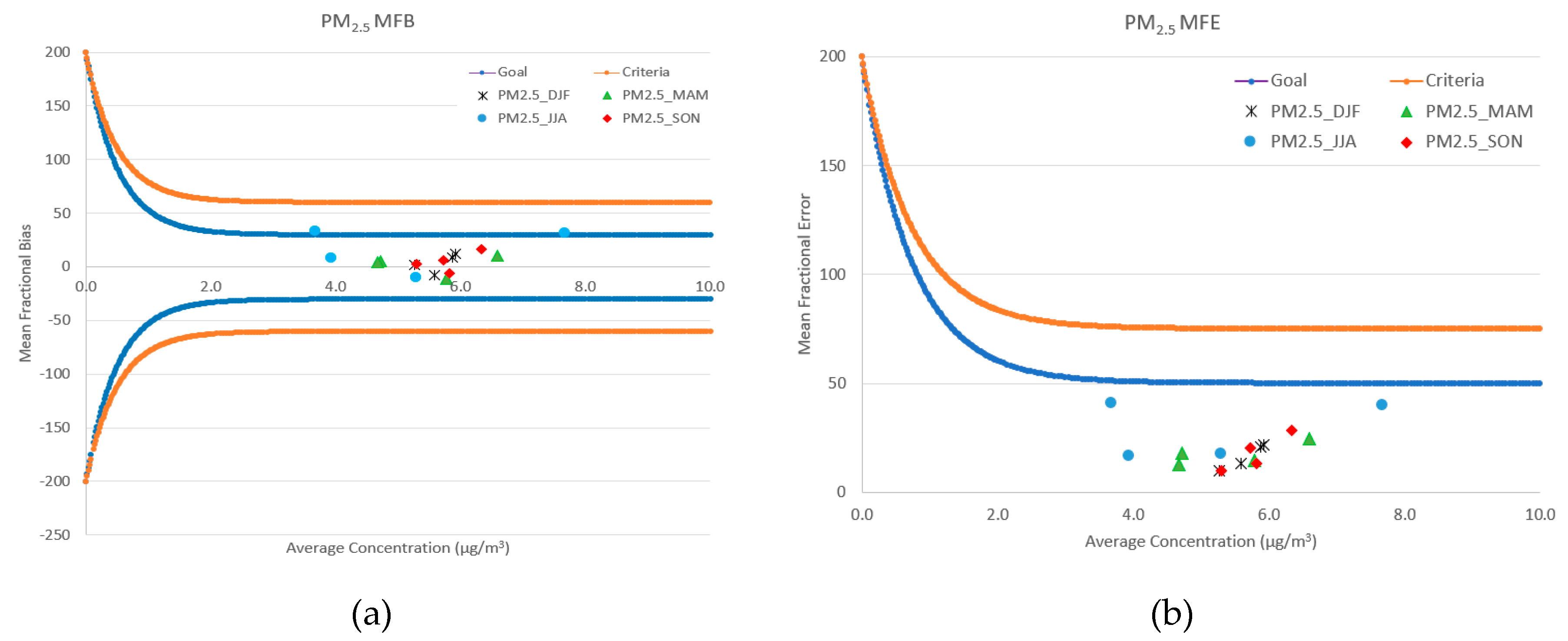
The exposure modelling conducted in this study was developed to assess population-weighted annual average PM_2.5 concentrations based on CCAM-CTM modelling predictions. This modelling supports the assessment of all-cause premature mortality due to long-term exposure to PM2.5 air pollution. Premature mortality has been found to be the most significant health endpoint from a health cost perspective, and a major driver of actions that reduce PM_2.5 health benefits due to the high monetary value allocated to a human statistical life [7,33,34].

The CCAM-CTM modelling results from 9-km CTM GMR domain were integrated by 3-km CTM GSYD domain (excluding 3-km CTM GSYD data from 9-km CTM GMR dataset). The model outputs were then re-gridded to a 1-km resolution to coincide the Australian Bureau of Statistics 1-km resolution gridded population data. For each 1-km grid in the NSW GMA shown with yellow boundary in Figure 2 (as defined in the Protection of the Environment Operations (Clean Air) Regulation 2010 as 57 Local Government Areas [35]), the modelled PM_2.5 concentration was multiplied by the usual residential population in that 1-km grid. The product was summed across all 1-km grid squares within the NSW GMA and divided by the total population calculated for the NSW GMA to get the population-weighted PM_2.5 concentration.

3. Model Evaluation

To assess CCAM-CTM model performance, modelled meteorology and PM_2.5 concentrations for calendar year of 2008 were compared to meteorological and PM_2.5 measurements from Bureau of Meteorology (BoM) automatic weather stations and NSW OEH air quality monitoring stations [36]. The PM_2.5 measurements were available only at five sites in 2008, namely, Chullora and Earlwood (Sydney East region), Richmond (Sydney Northwest region), Liverpool (Sydney Southwest region) and Wollongong (Illawarra region). The general guidance used in this evaluation referenced the procedure for model evaluation and benchmarking described in [22]. When evaluating modelled PM_2.5 projections, reference was made to the following performance metrics: mean bias (MB), normalised mean bias (NMB), mean fractional bias (MFB), mean error (ME), normalised mean error (NME), mean fractional error (MFE), root mean square error (RMSE), correlation coefficient (R), index of agreement (IOA) and overall skill (Skill_V), which was estimated by the ratio between standard deviation of predictions and observations (when it approached 1 shows skills in the model). The MB and ME assess general tendency and errors of model predictions. The NMB and NME normalise MB and ME by the mean of observations, and NMB ranges from −100% to +∞, while NME is from 0% to +∞. The MFB is defined as the bias normalized by the mean of paired predictions and observations, and the MFE is defined in a similar way. As proposed by [37], the model performance criteria is met when MFB and MFE is less or equal to ±60% and 75%, respectively. Model performance goal is further met when MFB and MFE is less or equal to ±30% and 50%. Model performance metrics were calculated and compared to other regional modelling study benchmarks as documented in [37,38,39,40].

The details of the CCAM performance evaluation are presented in Supplementary Materials. The air temperature was well represented by the CCAM simulation, in terms of the model was able to replicate observed seasonal and diurnal temperature variations. The modelled temperature was slightly warmer but within referenced benchmarks. The overall diurnal variations and seasonal patterns in the wind field were well represented by the model. Modelled wind speeds were slightly overpredicted but within reasonable limits of the expected performance of a mesoscale meteorological model. However, the CCAM simulation had a tendency to predict stronger winds in particular overnight. This could impact the model’s ability to accurately model the dispersion of pollutants and should be considered when assessing the performance of the chemical transport model.

Table 2. Quantitative performance statistics for predicted hourly PM_2.5 concentration (µg/m³) against observations for regions by seasons.

Seasons	Sub-Regions	Mean CTM	SD CTM	Mean Obs	SD Obs	MB	NMB	MFB	ME	NME	MFE	RMSE	r	IOA	SKILLv
Summer	Sydney East	5.9	2.6	5.4	3.7	0.7	0.14	12%	2.5	0.51	22%	3.5	0.46	0.54	0.71
	Sydney NW	5.6	2.6	7.5	4.0	−2.4	−0.32	−8%	3.4	0.50	13%	4.5	0.37	0.44	0.61
	Sydney SW	5.3	2.5	6.2	4.0	−0.4	−0.06	2%	2.6	0.45	10%	3.6	0.47	0.56	0.68
	Illawarra	5.9	2.8	6.1	4.4	0.2	0.03	9%	3.2	0.54	21%	4.3	0.34	0.53	0.63
Autumn	Sydney East	6.6	4.5	6.7	5.5	0.3	0.04	11%	3.4	0.51	25%	4.7	0.59	0.59	0.87
	Sydney NW	5.8	3.1	8.0	4.5	−3.5	−0.43	−11%	4.0	0.50	15%	5.5	0.32	0.40	0.45
	Sydney SW	4.7	2.4	6.6	5.5	−0.5	−0.07	5%	3.2	0.50	13%	4.8	0.52	0.61	0.62
	Illawarra	4.7	2.5	5.2	4.2	0.0	0.01	5%	2.8	0.54	18%	3.8	0.46	0.56	0.59
Winter	Sydney East	7.7	5.6	5.3	5.7	2.8	0.53	31%	5.0	0.94	40%	6.5	0.47	0.41	1.02
	Sydney NW	5.3	3.2	6.6	4.2	−3.0	−0.45	−10%	3.8	0.57	18%	5.3	0.09	0.40	0.44
	Sydney SW	3.9	2.1	6.5	6.1	−0.1	−0.01	8%	4.0	0.63	16%	5.4	0.49	0.57	0.62
	Illawarra	3.7	1.7	3.3	3.5	1.3	0.38	33%	2.9	0.89	41%	4.0	0.17	0.39	0.60
Spring	Sydney East	6.3	2.6	5.6	5.1	1.0	0.18	17%	3.7	0.66	28%	5.4	0.19	0.46	0.52
	Sydney NW	5.8	2.4	7.1	3.7	−2.0	−0.29	−6%	3.3	0.46	13%	4.4	0.17	0.40	0.54
	Sydney SW	5.3	2.2	6.5	7.5	−0.4	−0.06	3%	3.5	0.54	10%	7.5	0.18	0.51	0.35
	Illawarra	5.7	2.5	6.4	4.9	−0.2	−0.03	6%	3.5	0.55	20%	4.9	0.25	0.52	0.53

(NMBIOA > 0.6 or 0.8 < Skill_V < 1.2 is highlighted with red); CTM: Chemical transport model; SD: Standard deviation; Obs: observation; MB: mean bias; NMB: normalised mean bias; MFB: mean fractional bias; ME: mean error; NME: normalised mean error; MFE: mean fractional error; RMSE: root mean square error; R: correlation coefficient; IOA: index of agreement; SKILLv: overall skill.

summarises the seasonal quantitative performance statistics for the CTM predicted hourly PM_2.5 along with the mean and standard deviation of predicted values and observations for each region. The MB shows hourly PM_2.5 was generally over-predicted in the Sydney East region and under-predicted in Sydney Northwest and Southwest regions. A relatively high correlation coefficient (R > 0.50) and high IOA (>0.6) were found with PM_2.5 predictions in autumn in the Sydney East and Sydney Southwest regions. The values of Skill_V for the Sydney East region also fell within the values of 0.8 to 1.2 in autumn and winter, demonstrating good agreement for the observed and modelled standard deviations.

The bugle plots for hourly PM_2.5 for all predicted/observed pairs values across regions in different seasons are shown in Figure 3. Figure 3a shows all the PM_2.5 predictions across regions meet the performance criteria for MFB (±60%) for all seasons, and most of them were also able to meet the performance goal for MFB (±30%), except the MFB calculated for the Sydney East and Illawarra regions which were marginally above 30%. And as illustrated in Figure 3b, all the PM_2.5 predictions across regions and seasons meet the performance goal for MFE (50%) and the performance criteria for MFE (75%).

4. Results and Discussions

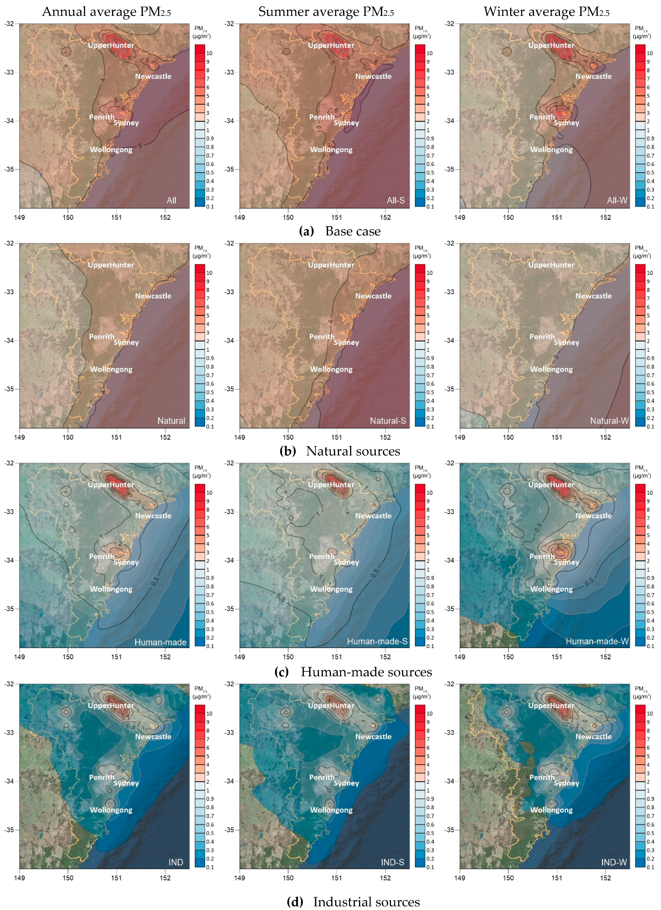
4.1. Predictied PM_2.5 Concentrations

The average PM_2.5 concentrations modelled for the CTM GMR domain (9-km × 9-km) for the entire calendar year of 2008, summer (December, January and February) and winter (June, July and August) for various modelling scenarios (as defined in Table 1) are illustrated in Figure 4.

The “base case” scenario depicts the areas of higher PM_2.5 concentrations which generally co-locates with populated areas, i.e., Sydney, Newcastle and Wollongong regions. Annual average PM_2.5 concentrations are below 7 µg/m³. PM_2.5 over the Sydney region is generally higher in winter. In Newcastle, PM_2.5 is higher in summer, while it does not vary much over Wollongong between seasons. Annual average PM_2.5 concentrations are modelled to exceed the Australian National Environment Protection Measures (NEPMs) ambient air quality standard of the annual average PM_2.5 of 8 µg/m³ over Upper Hunter region (areas of PM_2.5 greater than 8 µg/m³ are highlighted with the red contour in Figure 4a). The area of elevated PM_2.5 is consistent between summer and winter.

The contribution of natural sources including biogenic, sea salt and wind-blown dust emissions to the average PM_2.5 concentrations are shown in Figure 4b. Natural sources contribute 2–4 µg/m³ to the annual average PM_2.5 in land, 3–5 µg/m³ to the summer average PM_2.5 and less than 3 µg/m³ to the winter average PM_2.5, respectively. Contributions from human-made sources to average PM_2.5 concentrations are shown in Figure 4c, with localised elevated PM_2.5 concentrations generally coinciding with populated areas consistent with Base case predictions (Figure 4a). Human-made sources are predicted to contribute significantly to PM_2.5 concentrations in the Upper Hunter region (areas of PM_2.5 greater than 8 µg/m³ are highlighted with red contour in Figure 4c). They are also found to contribute significantly to localised elevated PM_2.5 in Sydney, Newcastle and Wollongong, with a greater extent projected in winter than summer.

Figure 4d–h depict the spatial distributions of contributions from several major human-made source groups defined in Table 1. Industry, which includes all other industrial sources except power generations from coal and gas was modelled to contribute significantly up 7 µg/m³ (and 8 µg/m³) to the summer (winter) average PM_2.5 concentrations in the Upper Hunter region (Figure 4d). PM_2.5 concentrations attributed to power station emissions are more elevated in localised regional areas coinciding with power station locations, and with contributions less than 1 µg/m³ to the annual average PM_2.5 shown in Figure 4e in those areas, with a slightly more contributions in summer than in winter. Contributions from power stations to average PM_2.5 are also modelled to be spatially dispersed over the NSW GMR due to emissions occurring from high stacks and the time taken for chemical transformation of precursors and secondary particle formation (Figure 4e). The major human-made sources contributed to annual average PM_2.5 in the Sydney region can be easily identified as wood heaters (Figure 4f) and on-road mobile vehicles (Figure 4g). The wood heaters obviously only have contributions to PM_2.5 concentrations in winter and they contribute up to 3 µg/m³ and 1 µg/m³ in the populated area of Sydney and Newcastle, respectively. Contributions to average PM_2.5 concentrations from on-road mobile vehicles appear slightly higher in winter in Sydney (0.5–0.6 µg/m³) compared to that in summer (0.4–0.5 µg/m³). It was suggested to attribute to more emissions from cold-start operations in winter and also a better dispersion condition with stronger winds and higher boundary layers predicted in summer. At last, apart from industrial sources, the non-road diesel and marine sources demonstrate relatively significant contributions up to 1 µg/m³ on average PM_2.5 concentrations in the Upper Hunter region (Figure 4h), and they also have 0.2 µg/m³ contributions to average PM_2.5 off the coastline near Sydney and Newcastle.

4.2. Major Chemical Components of PM_2.5

To quantify the temporal and spatial variations in major chemical components of PM_2.5, five key chemical species of PM_2.5, such as particulate nitrate, particulate sulphate, particulate ammonium, sodium and elemental carbon, as well as total PM_2.5 mass were extracted from CCAM-CTM model predictions in the CTM GMR domain (9-km × 9-km) for the entire calendar year of 2008 at eighteen NSW OEH air quality monitoring stations (shown as red dots in Figure 2) located in the Sydney East (Chullora, Earlwood, Lindfield, Randwick and Rozelle), Sydney Northwest (Prospect, Richmond, St Marys and Vineyard), Sydney Southwest (Bargo, Bringelly, Liverpool, Macarthur and Oakdale), Illawarra (Albion Park, Kembla Grange and Wollongong) and Newcastle (Newcastle) regions, respectively.

A regional average of total PM_2.5 concentrations and the major chemical species concentrations at each of the five regions for summer (December, January and February) and winter (June, July and August) in 2008 are shown in Figure 5. The regional average total PM_2.5 concentrations in summer are between 5.2–6.1 µg/m³, while the lowest PM_2.5 is found in the Sydney Southwest region and the highest one in the Newcastle region. Particulate sulphate contributes 0.79−0.95 µg/m³ (15–16%) to the total PM_2.5 mass, followed by sodium and particulate nitrate that account for 0.63–1.06 µg/m³ (12–18%) and 0.39–0.44 µg/m³ (7–8%) to the total PM_2.5 mass, respectively. Elemental carbon had less contribution to the total PM_2.5 mass (0.04–0.18 µg/m³ or 1–3%) compared to other species shown in Figure 5a, while ammonium also plays a very minor role (0.01–0.04 µg/m³ or less than 0.8% to the total PM_2.5 mass) in total PM_2.5 composition. The rest of other chemical species including primary and secondary organic aerosols, as well as chloride, calcium, magnesium, and potassium are integrated into the “other” category, as shown in Figure 5a, which account for around 60% (3.23–3.59 µg/m³) of the total PM_2.5 mass.

The regional average total PM_2.5 concentrations in winter shown in Figure 5b are generally lower than those in summer. The most significant drop of total PM_2.5 mass from summer to winter is found in the Illawarra region (2.17 µg/m³ or 38%). However, one exception with significant increase of total PM_2.5 mass is in the Sydney East region (1.77 µg/m³ or 30%), which is apparently related to the increase of concentrations of elemental carbon as well as “other” species (including primary and secondary organic aerosols) in the PM_2.5 compositions. The trend of increase in elemental carbon mass and decrease in particulate sulphate mass from summer to winter is clear at each of the five regions. The mass of sodium also decreases across regions from summer to winter although it still accounts for nearly 20% of total PM_2.5 mass in the Newcastle region. The rest of other chemical species (“other” category) has similar proportion around 60% to the total PM_2.5 mass.

Particulate nitrate, sulphate and ammonium are produced by chemical reactions in the atmosphere from gaseous precursors (e.g., NO₂ and SO₂ from human-made sources) and they are dominant species in secondary inorganic aerosols. The regional average of total mass of particulate nitrate, sulphate and ammonium across regions predicted in summer of 2008 were 1.22–1.39 µg/m³ and accounted for ~23% to the total PM_2.5 concentrations. The regional average secondary inorganic aerosols mass from our modelling results is slightly lower than what was found in Sydney Particle Characterisation Study, where the average mass of ammonium and sulphate was 1.61 µg/m³ [15]. The ratio between secondary inorganic aerosols to the total PM_2.5 mass in our study (23%) is close to what was found in chemical transport modelling works done in the Sydney Particle Study, which was around 20% in summer of 2011 [21], however it is significantly higher than the ratio of 15% estimated from field particle measurements conducted at the same time.

Sodium is a major marker specie for source of sea salt. The sea salt emissions from waves breaking in the open ocean and the coastal surf breaks are begin transported to coastal regions where sodium is found to be accounted for up to 18% of total PM_2.5 mass in the Newcastle and Illawarra region in both summer and winter in our study. The sodium contributions to the total PM_2.5 mass are slightly lower in the three sub-regions across Sydney (9–12%), while the ratio is very close to what was found in Sydney Particle Characterisation Study, where average chemical composition of salt was 12% for all four sites in Sydney [15]. It should be noted that chloride concentration has not been considered in this analysis and with that the contribution of sea salt to the total PM_2.5 discussed here may be underestimated.

The contributions from elemental carbon to total PM_2.5 mass in our study are generally below 5% in summer of 2008, and they are very close to the ratio of 6% estimated from field particle measurements conducted in summer of 2011 in the Sydney Particle Study [21]. The elemental carbon contributions to total PM_2.5 mass increased significantly from summer into winter in our study, especially in the Sydney East and Sydney Northwest regions. The elemental carbon contributions in both regions are below 3% in summer but increase up to 13% in winter. The findings are consistent with the increased wood heater usage in winter in populated areas across Sydney.

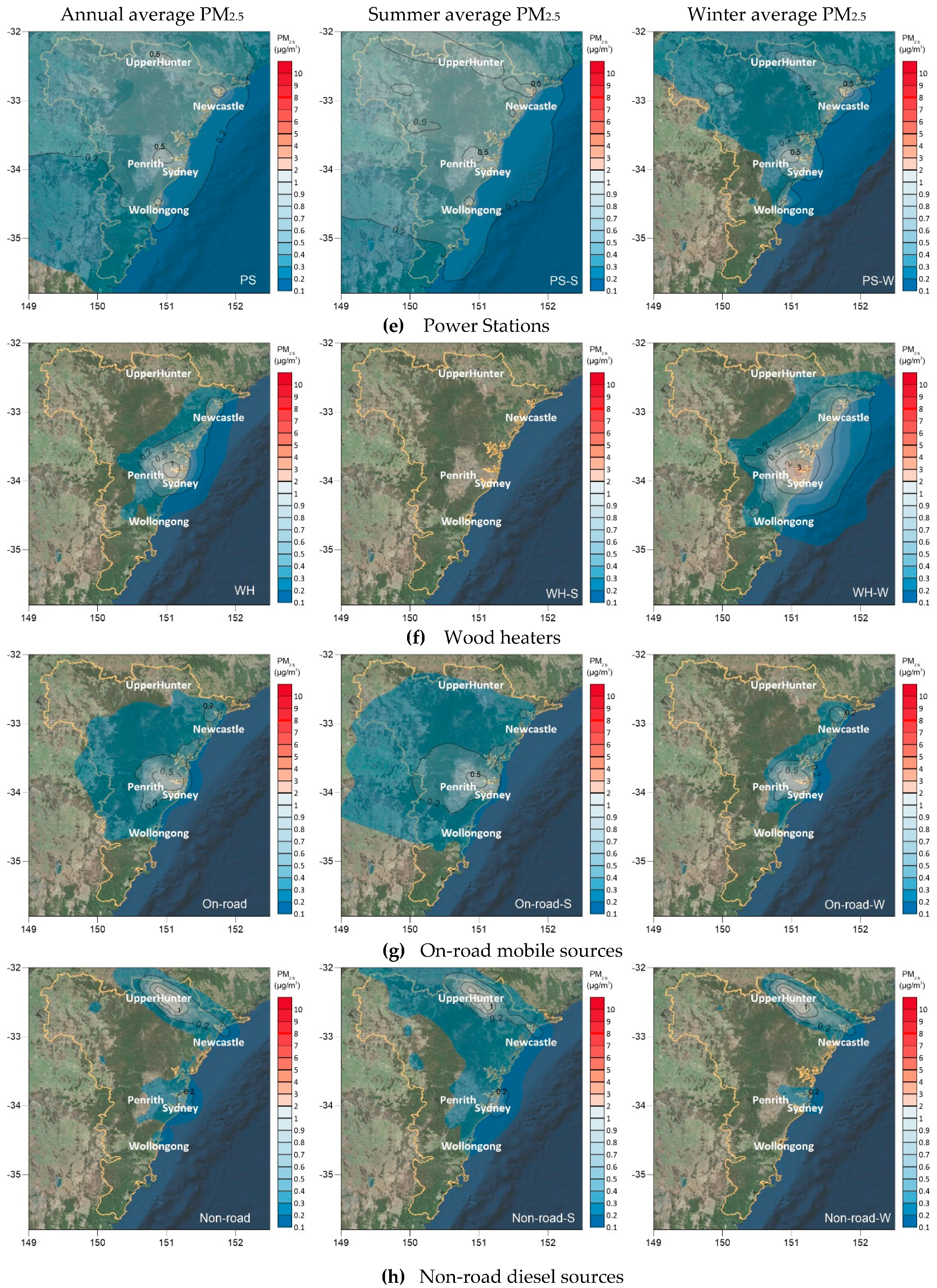
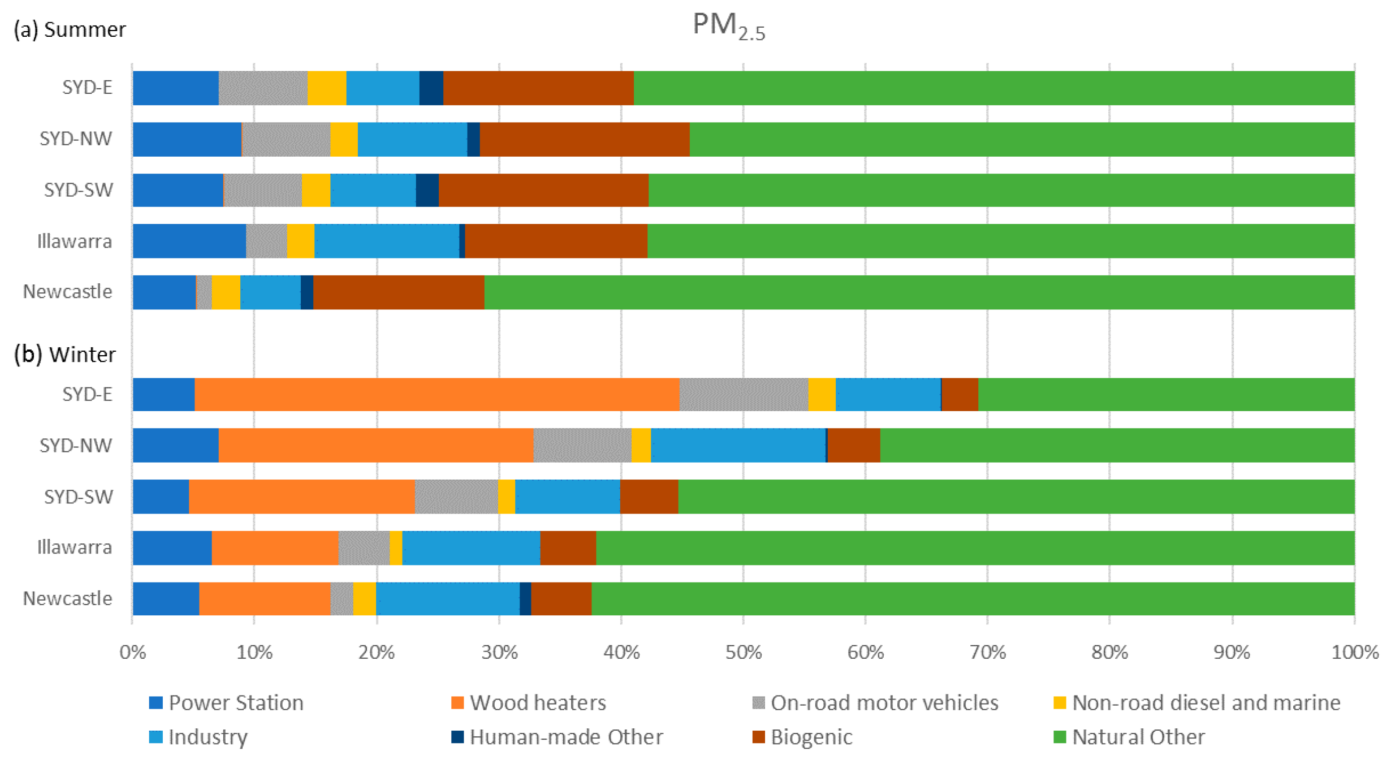
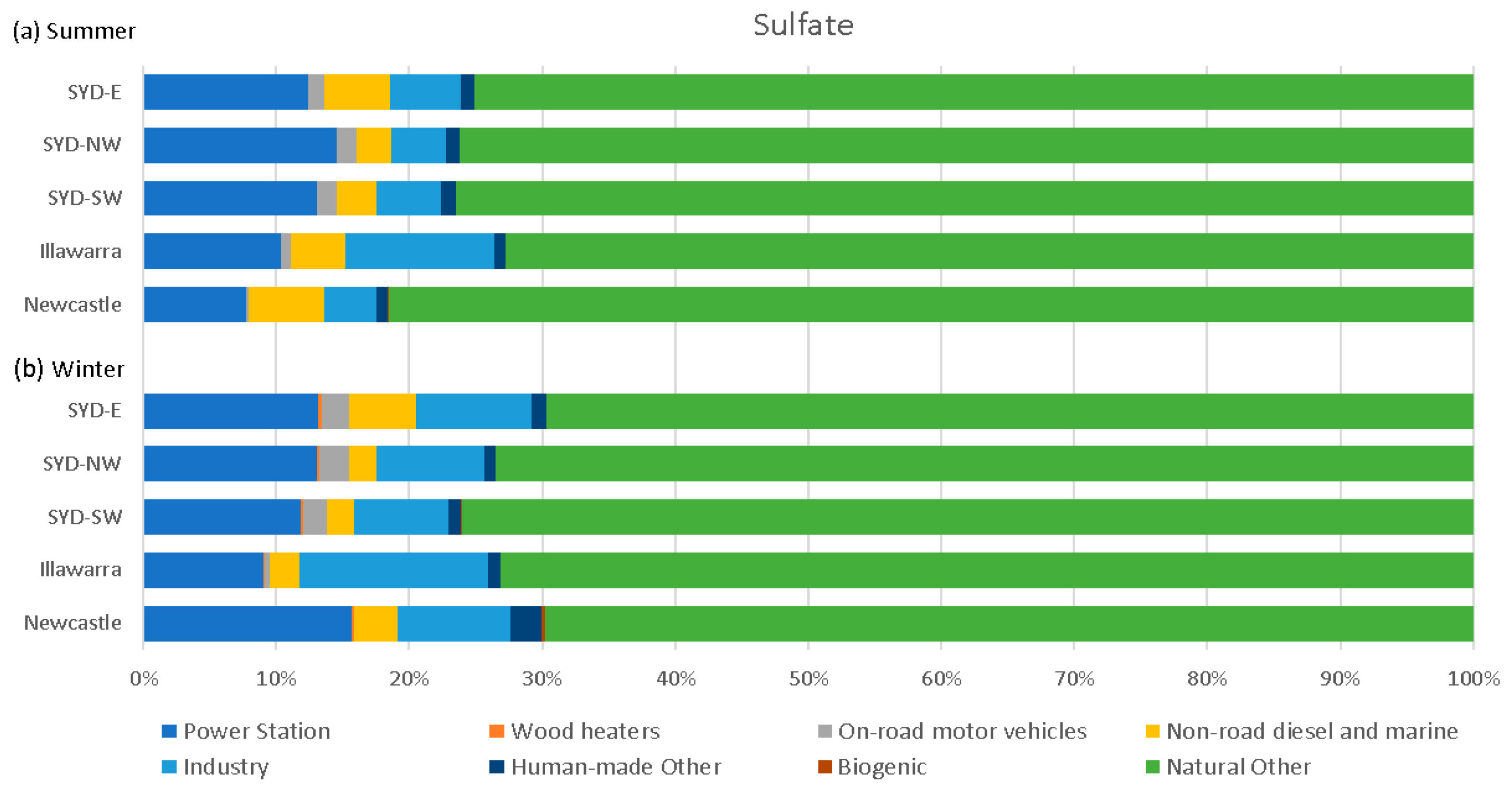
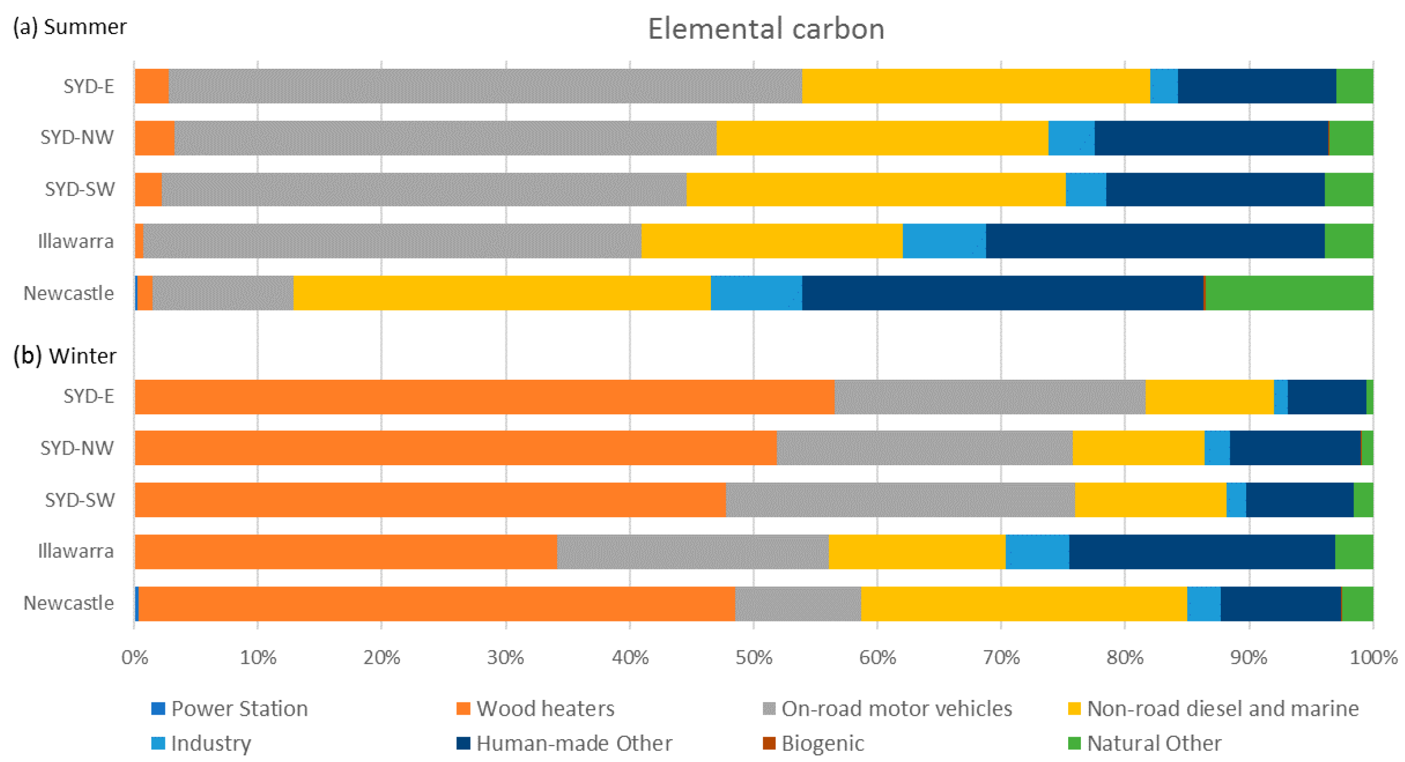
4.3. Source Contributions of PM_2.5

To investigate the major source contributions to the total PM_2.5 mass and the major chemical components discussed in Section 4.2, the predictions from CCAM-CTM modelling for the entire calendar year of 2008 under various modelling scenarios (as shown in Figure 4) are extracted at NSW OEH eighteen air quality monitoring stations across the Sydney East, Sydney Northwest, Sydney Southwest, Illawarra and Newcastle regions. The major source groups discussed in this section includes: power stations, wood heaters, on-road motor vehicles, non-road diesel and marine, industry, human-made other, biogenic and natural-other sources as their corresponding modelling scenarios listed in Table 1.

The regional average major source group contributions (%) to the total PM_2.5 mass at each of the five regions in summer and winter of 2008 is shown in Figure 6. In Figure 6a, the natural sources apparently dominate the contributions to the total PM_2.5 mass in summer of 2008. Biogenic and natural-other sources together contribute 71% to the total PM_2.5 mass in the Sydney Northwest region and up to 85% in the Newcastle region. Among human-made sources, power stations and on-road motor vehicles together contribute around 15% to the total PM_2.5 mass in three Sydney sub-regions. While the industry has larger contribution of 12% to the total PM_2.5 mass in the Illawarra region. Non-road diesel and marine generally has contribution less than 3% to the total PM_2.5 across regions. In winter of 2008, as shown in Figure 6b, natural sources are still the dominating contributors which contribute more than 60% to the total PM_2.5 mass in the Sydney Southwest, Illawarra and Newcastle regions. However, the wood heaters apparently make significant contributions and account for up to 40, 26 and 18% to total PM_2.5 mass in Sydney East, Sydney Northwest and Sydney Southwest regions, respectively in winter. Followed by the emissions from power stations and on-road motor vehicles that together contribute up to 16% of total PM_2.5 mass in winter. There is no significant change in average percentages of contributions from industrial sources (12–14%) and from non-road diesel and marine (3–5%) to total PM_2.5 mass between winter and summer.

The major source groups’ contributions to the secondary inorganic aerosols (including particulate nitrate, particulate sulphate and ammonium) are further illustrated in Figure 7, Figure 8 and Figure 9. In Figure 7, more than 40% of particulate nitrate mass come from human-made sources, while on-road motor vehicles and non-road diesel and marine certainly are the major sources among human-made sources that have greater contributions to particulate nitrate mass. Power stations have similar regional average contributions (below 5%) in most of the regions across summer and winter. Industry generally has more contributions across regions in winter than in summer.

In Figure 8, natural-other sources (including sea salt and wind-blown dust) contribute generally around 75% of particulate sulphate mass across regions in summer, while the contributions from natural-other sources slightly decrease in winter. Power stations and the industry are the two most significant contributors from human-made source groups, together they are found to be contributed to 25% of particulate sulphate mass in the Newcastle region in winter and 21–23% of sulphate mass in the Illawarra region. It is shown clearly in Figure 9 that human-made sources are the major sources of ammonium mass. More than 60% of ammonium mass are contributed from power stations and industry in summer across regions, while the relatively higher contributions from on-road motor vehicle are found in winter.

As shown in Figure 10a, it is obvious that on-road motor vehicles and non-road diesel and marine are the two major contributors to elemental carbon mass across regions in summer. Emissions from on-road motor vehicles play more important role in contribution of elemental carbon in three Sydney sub-regions and Illawarra, while non-road diesel and marine is the leading contributor of elemental carbon in the Newcastle. Emissions from wood heaters become a more significant source of elemental carbon in winter (Figure 10b), it contributes to 48–57% of elemental carbon mass across three Sydney sub-regions, while the regional average contribution percentage from on-road motor vehicles and non-road diesel and marine seem decrease compared to that in summer.

It is a challenge when comparing results from source-based methods in this study and from receptor-based methods (e.g., [9,14,15]) because of the mismatching in source categories. As summarised in

Table 3. The top three major source groups’ contributions (highlighted in red, blue and green, respectively) to total PM_2.5 mass, nitrate, sulphate, ammonium and elemental carbon at each of the five regions in NSW GMR.

Regions	Major Source Groups Contributions		Power Station	Wood Heaters	On-Road Motor Vehicles	Non-Road Diesel and Marine	Industry	Human-Made Other	Biogenic	Natural Other
Sydney East	PM2.5	summer	7%	0%	7%	3%	6%	2%	16%	59%
		winter	5%	40%	11%	2%	9%	0%	3%	31%
	Nitrate	summer	0%	0%	11%	3%	0%	26%	8%	51%
		winter	0%	2%	13%	0%	3%	24%	12%	45%
	Sulphate	summer	12%	0%	1%	5%	5%	1%	0%	75%
		winter	13%	0%	2%	5%	9%	1%	0%	70%
	Ammonium	summer	47%	0%	14%	13%	13%	2%	2%	9%
		winter	26%	6%	25%	16%	16%	2%	4%	5%
	EC	summer	0%	3%	51%	28%	2%	13%	0%	3%
		winter	0%	57%	25%	10%	1%	6%	0%	0%
Sydney NW	PM2.5	summer	9%	0%	7%	2%	9%	1%	17%	54%
		winter	7%	26%	8%	2%	14%	0%	4%	39%
	Nitrate	summer	2%	0%	18%	3%	0%	21%	4%	51%
		winter	1%	1%	15%	2%	4%	20%	8%	48%
	Sulphate	summer	15%	0%	1%	3%	4%	1%	0%	76%
		winter	13%	0%	2%	2%	8%	1%	0%	74%
	Ammonium	summer	38%	0%	11%	5%	16%	1%	2%	27%
		winter	24%	4%	23%	4%	31%	1%	4%	10%
	EC	summer	0%	3%	44%	27%	4%	19%	0%	4%
		winter	0%	52%	24%	11%	2%	11%	0%	1%
Sydney SW	PM2.5	summer	7%	0%	6%	2%	7%	2%	17%	58%
		winter	5%	18%	7%	1%	9%	0%	5%	55%
	Nitrate	summer	2%	0%	12%	3%	1%	25%	6%	52%
		winter	2%	1%	15%	3%	7%	17%	11%	45%
	Sulphate	summer	13%	0%	2%	3%	5%	1%	0%	77%
		winter	12%	0%	2%	2%	7%	1%	0%	76%
	Ammonium	summer	35%	0%	10%	7%	26%	1%	2%	19%
		winter	19%	2%	16%	4%	44%	1%	4%	9%
	EC	summer	0%	2%	42%	31%	3%	18%	0%	4%
		winter	0%	48%	28%	12%	2%	9%	0%	2%
Illawarra	PM2.5	summer	9%	0%	3%	2%	12%	0%	15%	58%
		winter	7%	10%	4%	1%	11%	0%	5%	62%
	Nitrate	summer	3%	0%	9%	7%	0%	22%	7%	53%
		winter	2%	1%	12%	3%	2%	16%	11%	54%
	Sulphate	summer	10%	0%	1%	4%	11%	1%	0%	73%
		winter	9%	0%	0%	2%	14%	1%	0%	73%
	Ammonium	summer	33%	0%	9%	11%	32%	2%	2%	10%
		winter	20%	3%	15%	4%	33%	4%	4%	17%
	EC	summer	0%	1%	40%	21%	7%	27%	0%	4%
		winter	0%	34%	22%	14%	5%	21%	0%	3%
Newcastle	PM2.5	summer	5%	0%	1%	2%	5%	1%	14%	71%
		winter	6%	11%	2%	2%	12%	1%	5%	62%
	Nitrate	summer	5%	0%	5%	9%	2%	24%	4%	51%
		winter	3%	1%	13%	4%	1%	16%	12%	50%
	Sulphate	summer	8%	0%	0%	6%	4%	1%	0%	82%
		winter	16%	0%	0%	3%	9%	2%	0%	70%
	Ammonium	summer	45%	0%	5%	12%	25%	4%	4%	6%
		winter	46%	5%	12%	4%	21%	2%	8%	2%
	EC	summer	0%	1%	11%	34%	7%	32%	0%	13%
		winter	0%	48%	10%	26%	3%	10%	0%	3%

, the top three major source groups contributed to total PM_2.5 mass, particulate nitrate, particulate sulphate, ammonium and elemental carbon at each of the five regions in the NSW GMR are highlighted in order with red, blue and green, it become obvious that apart from natural sources (“biogenic” plus “natural-other” source groups), “power station” is the first or second major source contributing to sulphate and ammonium mass in both summer and winter across regions, and it is also generally the third major contributors to the total PM_2.5 mass in summer. “Wood heaters” is the first or second major source contributing to total PM_2.5 and EC mass across three Sydney sub-regions in winter. “On-road mobile vehicles” is the top contributor to EC mass across regions, and it also has significant contributions to total PM_2.5 mass, particulate nitrate and sulphate mass in the Sydney East region. “Non-road diesel and marine” plays a relatively important role in EC mass across regions except Illawarra. Similar results are also found with “industry”, which is the first or second major contributors to sulphate and ammonium mass across regions, it is also the second or third major contributor to total PM_2.5 mass across regions.

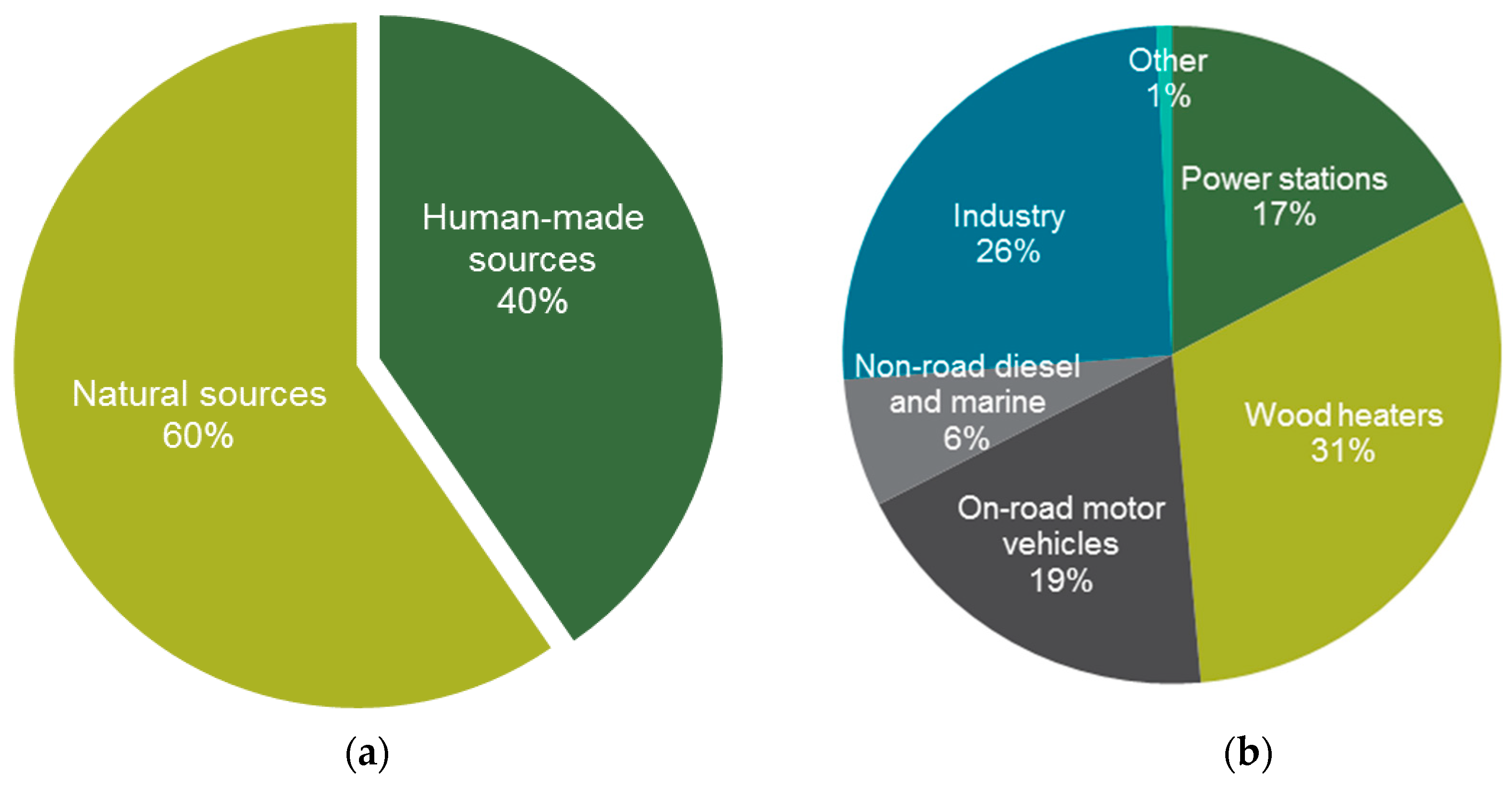
4.4. Population-Weighted Annual PM_2.5 Concentrations

The CCAM-CTM modelling results from various emission scenarios discussed in Section 4.1 were applied to the method described in Section 2.3 to estimate the major source contributions to population-weighted annual average PM_2.5. As summarised in Figure 11a and

Table 4. Natural and major human-made sources contributions to population-weighted annual average PM_2.5 concentrations.

Sources	Population-Weighted Annual Average PM2.5 (µg/m³)
Natural	3.55
Human-made	Power stations	0.42		2.41
	Wood heaters	0.75
	On-road motor vehicles	0.46
	Non-road diesel and marine	0.15
	Industry	0.61
	Other	0.02
All	5.96

, the natural and human-made sources contribute 60% (3.55 µg/m³) and 40% (2.41 µg/m³) to the population-weighted annual average PM_2.5 (5.96 µg/m³). The contributions from total human-made sources were further broken down into major source groups, i.e., wood heaters, industry, on-road motor vehicles, power stations and non-road diesel and marine as shown in Figure 11b, while each of these major source groups contributed 0.75, 0.61, 0.46, 0.42 and 0.15 µg/m³ to population-weighted annual average PM_2.5 and accounted for 31%, 26%, 19%, 17% and 6% in the total human-made sources contribution (40% in Figure 11a).

The population of our study region (shown as NSW GMA in Figure 2) was about 5.25 million in 2016 and densely populated in Sydney, Newcastle and Wollongong. Exposure to ambient air pollution is a major risk factor for global disease. From the study of Brauer et al. [41], 87% of the world’s population lived in areas exceeding the World Health Organization Air Quality Guideline of 10 μg/m³ PM_2.5 (annual average) in 2013, however, the decreases in population-weighted mean concentrations of PM_2.5 were evident in most of high income countries between 1990 and 2013. Australia was among one of those country who had the lowest country-level population-weighted estimates of ≤6 μg/m³. The population-weighted annual average PM_2.5 modelled for 2008 in the NSW GMA was 5.96 µg/m³ from our study, slightly lower than the most recent value for PM_2.5 mean annual exposure in Australia was 6.126 µg/m³ as of 2016 [42] based on the methods discussed in [41]. The exposure modelling work presented in this section provides quantitatively estimation of the amount of PM_2.5 that people were exposed to. Results from exposure modelling are also a critical component and primary inputs to for health impact assessment (HIA).

5. Conclusions

The CCAM-CTM modelling system had been configured and applied to predict ambient PM_2.5 in the NSW GMR for 2008 calendar year. The CCAM-CTM was undertaken with eleven emission scenarios embedded with sixteen major source groups which were segregated from the 2008 NSW GMR Air Emission Inventory. Model results were analysed to characterise spatio-temporal variations in PM_2.5 concentrations for the NSW GMR. They were also used to quantity the relative contributions of major human-made sources (power stations, wood heaters, on-road motor vehicles, non-road diesel and marine and industry) to PM_2.5 concentrations and the major chemical components of PM_2.5 (sulphate, nitrate, ammonium, elemental carbon and sodium). By multiplying modelled concentrations with Australian Bureau of Statistics 1km resolution gridded population data, the major source contributions to the population-weighted annual average PM_2.5 concentrations were further estimated. The major findings of this study are summarised as follows:

• Populated areas in the NSW GMR (Sydney, Newcastle and Wollongong) are characterised with annual average PM_2.5 of 6–7 µg/m³. Natural sources including biogenic emissions, sea salt and wind-blown dust contributed 2–4 µg/m³ to the annual average PM_2.5 in these regions.
• Annual average PM_2.5 is modelled to exceed 8 µg/m³ in the Upper Hunter region, while two major source groups, namely “industry” and “non-road diesel and marine “are identified to contribute up to 7 and 1 µg/m³ on annual average PM_2.5 concentrations in this region, respectively.
• Seasonal variations in regional PM_2.5 concentrations are found across Sydney-East, Sydney Northwest, Sydney Southwest, Illawarra and Newcastle regions. Summer and winter regional PM_2.5 concentrations range from 5.2–6.1 µg/m³ and 3.7–7.7 µg/m³, respectively. The regional total mass of predicted secondary inorganic aerosols (particulate nitrate, sulphate and ammonium) are between 1.22–1.39 µg/m³, and their ratio to the total PM_2.5 mass is 23%. Sodium accounts for up to 18% of total PM_2.5 mass in the Newcastle and Illawarra region in both summer and winter. The significant increase in EC mass from summer (0.18 µg/m³) to winter (0.97 µg/m³) is found in Sydney East region, and similar results are also found in other regions.
• Apart from natural sources, “Power stations” is identified to be the third major contributor to the summer total PM_2.5 mass across regions, and the first or second contributor to sulphate and ammonium mass in both summer and winter. “Wood heaters” is the first or second major source contributing to total PM_2.5 and EC mass across three Sydney sub-regions in winter. “On-road mobile vehicles” is the top contributor to EC mass across regions, and it also has significant contributions to total PM_2.5 mass, particulate nitrate and sulphate mass in the Sydney East region. “Non-road diesel and marine” plays a relatively important role in EC mass across regions except Illawarra. “Industry” is the first or second major contributor to sulphate and ammonium mass, and it is also the second or third major contributor to total PM_2.5 mass across regions.
• The natural and human-made sources contribute 60% (3.55 µg/m³) and 40% (2.41 µg/m³) to the population-weighted annual average PM_2.5 (5.96 µg/m³). Major source groups as “wood heaters”, “industry”, “on-road motor vehicles”, “power stations” and “non-road diesel and marine” accounts for 31%, 26%, 19%, 17% and 6% in the total human-made sources contribution, respectively.

The PM_2.5 levels in NSW are relatively low among industrialised countries and considered good by international standards. However, even at low levels, the PM_2.5 still has significant impact on human health and the economy of the state. Long-term, large population exposures to PM_2.5 concentrations account for a significant portion of the health costs associated with air pollution exposures within the NSW GMR. Reducing PM_2.5 levels by even a small amount will reduce the number of premature deaths and hospital admissions. The results from this study demonstrate the success of the systematic approach using regional airshed modelling to investigate major source contributions to regional PM_2.5, and this approach certainly can be applied to any other regions where suffer from severe PM_2.5 pollution. A quantitative understanding of major sources contributions to PM_2.5 and the exposures also provides the key messages for government agencies to consider while making evidence-based policies aiming to deliver improved public outcomes.

References

1. Fann, N.; Lamson, A.D.; Anenberg, S.C.; Wesson, K.; Risley, D.; Hubbell, B.J. Estimating the National Public Health Burden Associated with Exposure to Ambient Pm2.5 and Ozone. Risk Anal. 2012, 32, 81–95. [Google Scholar] [CrossRef] [PubMed]
2. Chen, Y.; Ebenstein, A.; Greenstone, M.; Li, H. Evidence on the Impact of Sustained Exposure to Air Pollution on Life Expectancy from China’s Huai River Policy. Proc. Natl. Acad. Sci. USA 2013, 110, 12936–12941. [Google Scholar] [CrossRef] [PubMed]
3. Xing, Y.-F.; Xu, Y.-H.; Shi, M.-H.; Lian, Y.-X. The Impact of Pm2.5 on the Human Respiratory System. J. Thorac. Dis. 2016, 8, E69–E74. [Google Scholar] [PubMed]
4. Du, Y.; Xu, X.; Chu, M.; Guo, Y.; Wang, J. Air Particulate Matter and Cardiovascular Disease: The Epidemiological, Biomedical and Clinical Evidence. J. Thorac. Dis. 2016, 8, E8–E19. [Google Scholar] [PubMed]
5. Laurent, O.; Hu, J.; Li, L.; Cockburn, M.; Escobedo, L.; Kleeman, M.J.; Wu, J. Sources and Contents of Air Pollution Affecting Term Low Birth Weight in Los Angeles County, California, 2001–2008. Environ. Res. 2014, 134, 488–495. [Google Scholar] [CrossRef] [PubMed]
6. NSW-OEH. Air Quality in Nsw. In Clean Air Summit; NSW-OEH: Sydney, Australia, 2017. [Google Scholar]
7. Broome, R.A.; Fann, N.; Cristina, T.J.N.; Fulcher, C.; Duc, H.; Morgan, G.G. The Health Benefits of Reducing Air Pollution in Sydney, Australia. Environ. Res. 2015, 143, 19–25. [Google Scholar] [CrossRef] [PubMed]
8. WHO. Review of Evidence on Health Aspects of Air Pollution—Revihaap Project; World Health Organization (WHO): Copenhagen, Denmark, 2013. [Google Scholar]
9. Hibberd, M.F.; Keywood, M.D.; Selleck, P.W.; Cohen, D.D.; Stelcer, E.; Scorgie, Y.; Chang, L.T.-C. Lower Hunter Particle Characterisation Study; NSW Environment Protection Authority: Sydney, Australia, 2016; p. 194.
10. NSW-EPA. 2008 Calendar Year Air Emissions Inventory for the Greater Metropolitan Region in Nsw; NSW-EPA: Sydney, Australia, 2012.
11. NSW-OEH. Towards Cleaner Air. Nsw Air Quality Statement 2016; NSW-OEH: Sydney, Australia, 2016.
12. Hopke, P.K. The Use of Source Apportionment for Air Quality Management and Health Assessments. J. Toxicol. Environ. Health Part A 2008, 71, 555–563. [Google Scholar] [CrossRef]
13. Burr, M.J.; Zhang, Y. Source Apportionment of Fine Particulate Matter over the Eastern U.S. Part I: Source Sensitivity Simulations Using Cmaq with the Brute Force Method. Atmos. Pollut. Res. 2011, 2, 300–317. [Google Scholar] [CrossRef]
14. Hibberd, M.; Selleck, P.; Keywood, M.; Cohen, D.; Stelcer, E.; Atanacio, A. Upper Hunter Valley Particle Characterization Study; CSIRO: Canberra, Australia, 2013; p. 72. [Google Scholar]
15. Cohen, D.D.; Atanacio, A.J.; Stelcer, E.; Garton, D. Sydney Particle Characterisation Study 2016; Australian Nuclear Science and Technology Organisation (ANSTO): Sydney, Australia, 2016; p. 156.
16. Marmur, A.; Unal, A.; Mulholland, J.A.; Russell, A.G. Optimization-Based Source Apportionment of Pm2.5 Incorporating Gas-to-Particle Ratios. Environ. Sci. Technol. 2005, 39, 3245–3254. [Google Scholar] [CrossRef]
17. Thompson, T.M.; Shepherd, D.; Stacy, A.; Barna, M.G.; Schichtel, B.A. Modeling to Evaluate Contribution of Oil and Gas Emissions to Air Pollution. J. Air Waste Manag. Assoc. 2017, 67, 445–461. [Google Scholar] [CrossRef]
18. Pun, B.K.; Seigneur, C.; Bailey, E.M.; Gautney, L.L.; Douglas, S.G.; Haney, J.L.; Kumar, N. Response of Atmospheric Particulate Matter to Changes in Precursor Emissions: A Comparison of Three Air Quality Models. Environ. Sci. Technol. 2008, 42, 831–837. [Google Scholar] [CrossRef] [PubMed]
19. Koo, B.; Wilson, G.M.; Morris, R.E.; Dunker, A.M.; Yarwood, G. Comparison of Source Apportionment and Sensitivity Analysis in a Particulate Matter Air Quality Model. Environ. Sci. Technol. 2009, 43, 6669–6675. [Google Scholar] [CrossRef] [PubMed]
20. Li, X.; Zhang, Q.; Zhang, Y.; Zheng, B.; Wang, K.; Chen, Y.; Wallington, T.J.; Han, W.; Shen, W.; Zhang, X.; et al. Source Contributions of Urban Pm2.5 in the Beijing–Tianjin–Hebei Region: Changes between 2006 and 2013 and Relative Impacts of Emissions and Meteorology. Atmos. Environ. 2015, 123 Pt A, 229–239. [Google Scholar] [CrossRef]
21. Cope, M.; Keywood, M.; Emmerson, K.; Galbally, I.; Boast, K.; Chambers, S.; Cheng, M.; Crumeyrolle, S.; Dunne, E.; Fedele, R.; et al. Sydney Particle Study; CSIRO: Canberra, Australia, 2014; p. 151. [Google Scholar]
22. Chang, L.T.-C.; Duc, H.; Scorgie, Y.; Trieu, T.; Monk, K.; Jiang, N. Performance Evaluation of Ccam-Ctm Regional Airshed Modelling for the New South Wales Greater Metropolitan Region. Atmosphere 2018, 9, 486. [Google Scholar] [CrossRef]
23. Duc, H.N.; Chang, L.; Trieu, T.; Salter, D.; Scorgie, Y. Source Contributions to Ozone Formation in the New South Wales Greater Metropolitan Region, Australia. Atmosphere 2018, 9, 443. [Google Scholar]
24. Hu, J.; Zhang, H.; Ying, Q.; Chen, S.H.; Vandenberghe, F.; Kleeman, M.J. Long-Term Particulate Matter Modeling for Health Effect Studies in California—Part 1: Model Performance on Temporal and Spatial Variations. Atmos. Chem. Phys. 2015, 15, 3445–3461. [Google Scholar] [CrossRef]
25. Buonocore, J.J.; Dong, X.; Spengler, J.D.; Fu, J.S.; Levy, J.I. Using the Community Multiscale Air Quality (Cmaq) Model to Estimate Public Health Impacts of Pm2.5 from Individual Power Plants. Environ. Int. 2014, 68, 200–208. [Google Scholar] [CrossRef] [PubMed]
26. McGregor, J.L. C-Cam Geometric Aspects and Dynamical Formulation; CSIRO: Canberra, Australia, 2005; p. 43. [Google Scholar]
27. Cope, M.E.; Hess, G.D.; Lee, S.; Tory, K.; Azzi, M.; Carras, J.; Lilley, W.; Manins, P.C.; Nelson, P.; Ng, L.; et al. The Australian Air Quality Forecasting System. Part I: Project Description and Early Outcomes. J. Appl. Meteorol. 2004, 43, 649–662. [Google Scholar] [CrossRef]
28. Sarwar, G.; Luecken, D.; Yarwood, G.; Whitten, G.Z.; Carter, W.P.L. Impact of an Updated Carbon Bond Mechanism on Predictions from the Cmaq Modeling System: Preliminary Assessment. J. Appl. Meteorol. Climatol. 2008, 47, 3–14. [Google Scholar] [CrossRef]
29. Sarwar, G.; Appel, K.W.; Carlton, A.G.; Mathur, R.; Schere, K.; Zhang, R.; Majeed, M.A. Impact of a New Condensed Toluene Mechanism on Air Quality Model Predictions in the US. Geosci. Model Dev. 2011, 4, 183–193. [Google Scholar] [CrossRef]
30. Fountoukis, C.; Nenes, A. Isorropia II: A Computationally Efficient Thermodynamic Equilibrium Model for K+–Ca2+–Mg2+–Nh4+–Na+–So42−–No3–Cl–H2o Aerosols. Atmos. Chem. Phys. 2007, 7, 4639–4659. [Google Scholar] [CrossRef]
31. Donahue, N.M.; Robinson, A.L.; Stanier, C.O.; Pandis, S.N. Coupled Partitioning, Dilution, and Chemical Aging of Semivolatile Organics. Environ. Sci. Technol. 2006, 40, 2635–2643. [Google Scholar] [CrossRef] [PubMed]
32. Cope, M.; Lee, S.; Noonan, J.; Lilley, B.; Hess, D.; Azzi, M. Chemical Transport Model—Technical Description; CSIRO: Canberra, Australia, 2009; p. 114. [Google Scholar]
33. Boulter, P.; Kulkarni, K. Economic Analysis to Inform the National Plan for Clean Air (Particles); Pacific Environment: Sydney, Australia, 2013.
34. US-EPA. The Benefits and Costs of the Clean Air Act from 1990 to 2020: Summary Report; US-EPA: Sydney, Australia, 2011. [Google Scholar]
35. Protection of the Environment Operations (Clean Air) Regulation. 2010. Available online: http://www.legislation.nsw.gov.au/#/view/regulation/2010/428/part1/sec3 (accessed on 12 March 2019).
36. NSW OEH Air Quality Monitoring Stations. Available online: https://www.environment.nsw.gov.au/topics/air/monitoring-air-quality/ (accessed on 12 March 2019).
37. Boylan, J.W.; Russell, A.G. Pm and Light Extinction Model Performance Metrics, Goals, and Criteria for Three-Dimensional Air Quality Models. Atmos. Environ. 2006, 40, 4946–4959. [Google Scholar] [CrossRef]
38. Chang, J.C.; Hanna, S.R. Air Quality Model Performance Evaluation. Meteorol. Atmos. Phys. 2004, 87, 167–196. [Google Scholar] [CrossRef]
39. Rao, S.T.; Galmarini, S.; Puckett, K. Air Quality Model Evaluation International Initiative (Aqmeii): Advancing the State of the Science in Regional Photochemical Modeling and Its Applications. Bull. Am. Meteorol. Soc. 2010, 92, 23–30. [Google Scholar] [CrossRef]
40. Morris, R.E.; McNally, D.E.; Tesche, T.W.; Tonnesen, G.; Boylan, J.W.; Brewer, P. Preliminary Evaluation of the Community Multiscale Air Quality Model for 2002 over the Southeastern United States. J. Air Waste Manag. Assoc. 2005, 55, 1694–1708. [Google Scholar] [CrossRef] [PubMed] [Green Version]
41. Brauer, M.; Freedman, G.; Frostad, J.; van Donkelaar, A.; Martin, R.V.; Dentener, F.; Dingenen, R.V.; Estep, K.; Amini, H.; Apte, J.S.; et al. Ambient Air Pollution Exposure Estimation for the Global Burden of Disease 2013. Environ. Sci. Technol. 2016, 50, 79–88. [Google Scholar] [CrossRef]
42. PM2.5 Air Pollution, Mean Annual Exposure. Available online: https://data.worldbank.org/indicator/EN.ATM.PM25.MC.M3?locations=AU (accessed on 12 March 2019).
Figure 1. Schematic diagram of the CCAM-CTM modelling system.
Atmosphere 10 00138 g001
Figure 2. Modelling domains for the NSW Greater Metropolitan Region (CTM GMR) and Greater Sydney (CTM GSYD). The NSW Greater Metropolitan Area (NSW GMA) domain (as defined in the Clean Air Regulation 2010) is also shown, and locations of NSW air quality monitoring stations referenced in the study are identified with red dots.
Atmosphere 10 00138 g002
Figure 3. Bugle plots (a) mean fractional bias (MFB) and (b) mean fractional error (MFE) for PM2.5 for all predicted/observed pairs values in the Sydney East, Sydney Northwest, Sydney Southwest and Illawarra regions for summer (DJF, black asterisk), autumn (MAM, green triangle), winter (JJA, blue dot) and spring (SON, red diamond). The benchmark criteria (orange lines) and goal (blue lines) for assessing the model performance, as defined by [37], are also shown.
Atmosphere 10 00138 g003
Figure 4. Average PM2.5 concentrations (µg/m3) in calendar year for 2008, summer (DJF) and winter (JJA) predicted by CCAM-CTM under different modelling scenarios: (a) base case, (b) natural sources, (c) human-made sources, (d) industrial sources, (e) power stations, (f) wood heaters, (g) on-road mobile sources and (h) non-road diesel sources. Area with source contribution greater than 8 µg/m3 is highlighted with red contour.
Atmosphere 10 00138 g004aAtmosphere 10 00138 g004b
Figure 5. Regional average concentrations of total PM2.5 (values shown on top of each stacked column), particulate nitrate (ANO3), ammonium (ANH4), sulphate (ASO4), sodium (SOD), elemental carbon (EC) and other species in the Sydney east (SYD-E), Sydney Northwest (SYD-NW), Sydney Southwest (SYD-SW), Illawarra and Newcastle regions for (a) summer and (b) winter in 2008.
Atmosphere 10 00138 g005
Figure 6. Regional average major source groups contribution (%) to total PM2.5 mass in the Sydney East (SYD-E), Sydney Northwest (SYD-NW), Sydney Southwest (SYD-SW), Illawarra and Newcastle regions in (a) summer and (b) winter of 2008.
Atmosphere 10 00138 g006
Figure 7. Regional average major source groups contribution (%) to particulate nitrate mass in the Sydney East (SYD-E), Sydney Northwest (SYD-NW), Sydney Southwest (SYD-SW), Illawarra and Newcastle regions in (a) summer and (b) winter of 2008.
Atmosphere 10 00138 g007
Figure 8. Regional average major source groups contribution (%) to particulate sulphate mass in the Sydney East (SYD-E), Sydney Northwest (SYD-NW), Sydney Southwest (SYD-SW), Illawarra and Newcastle regions in (a) summer and (b) winter of 2008.
Atmosphere 10 00138 g008
Figure 9. Regional average major source groups contribution (%) to ammonium mass in the Sydney East (SYD-E), Sydney Northwest (SYD-NW), Sydney Southwest (SYD-SW), Illawarra and Newcastle regions in (a) summer and (b) winter of 2008.
Atmosphere 10 00138 g009
Figure 10. Regional average major source groups contribution (%) to elemental carbon mass in the Sydney East (SYD-E), Sydney Northwest (SYD-NW), Sydney Southwest (SYD-SW), Illawarra and Newcastle regions in (a) summer and (b) winter of 2008.
Atmosphere 10 00138 g010
Figure 11. (a) Natural and human-made sources contributions (%) to population-weighted annual average PM2.5 (b) major source groups contributions (%) to total human-made sources contribution (40% in (a)).
Atmosphere 10 00138 g011