New Interpretative Scales for Lichen Bioaccumulation Data: The Italian Proposal

 , ,
, ,  , ,
, ,  ,
,  ,
,  , ,
, , 
 ,
,  and
and
Abstract
1. Introduction
2. Data and Methodology
2.1. Data Collection
2.2. Data Processing
2.3. Working Examples: Case Studies from NE Italy
3. Results and Discussion
3.1. Native Lichens
3.1.1. Source Data and Species-Specific BECs
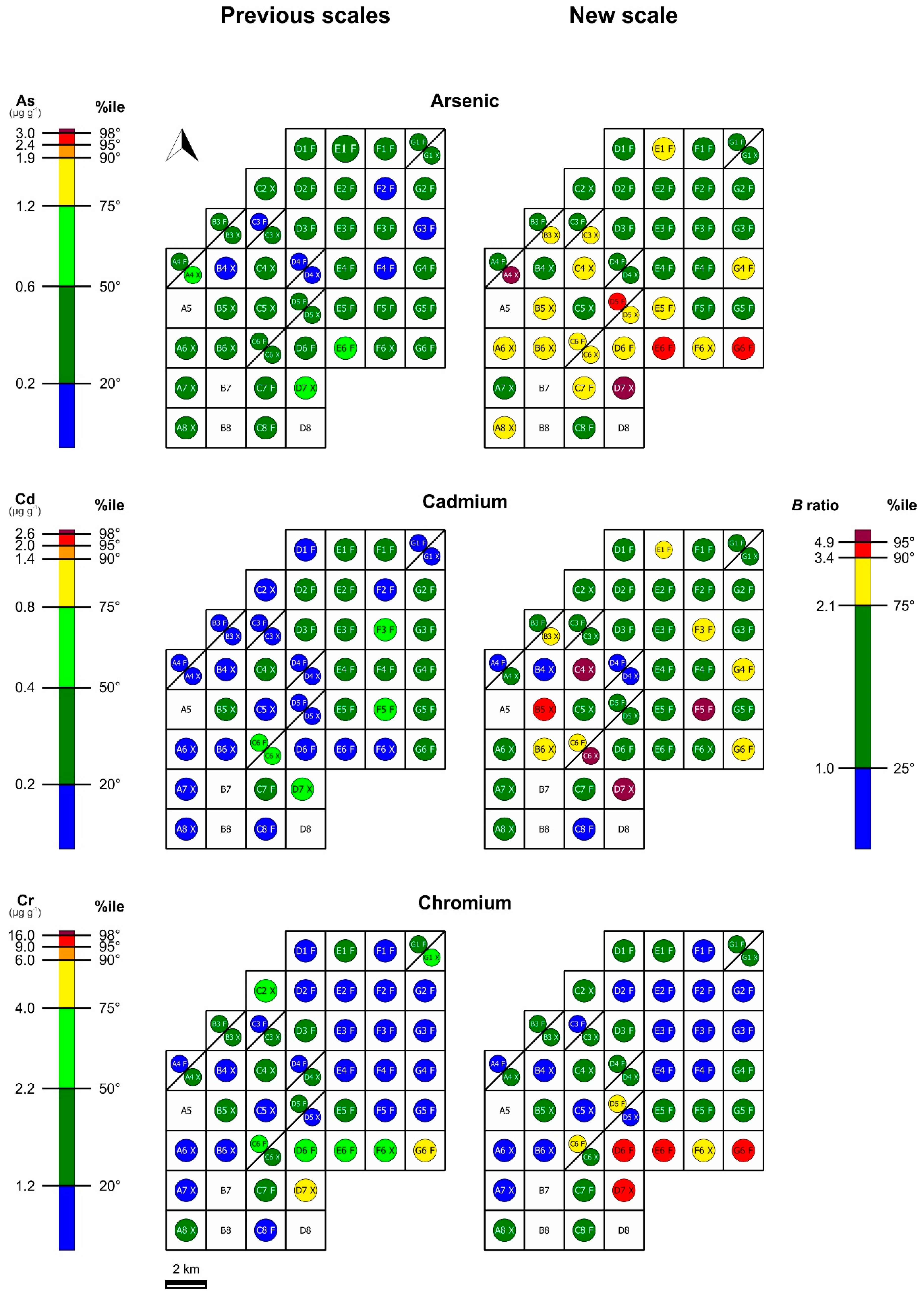
3.1.2. Bioaccumulation Scale for Native Lichens
3.2. Lichen Transplants
3.2.1. Source Data
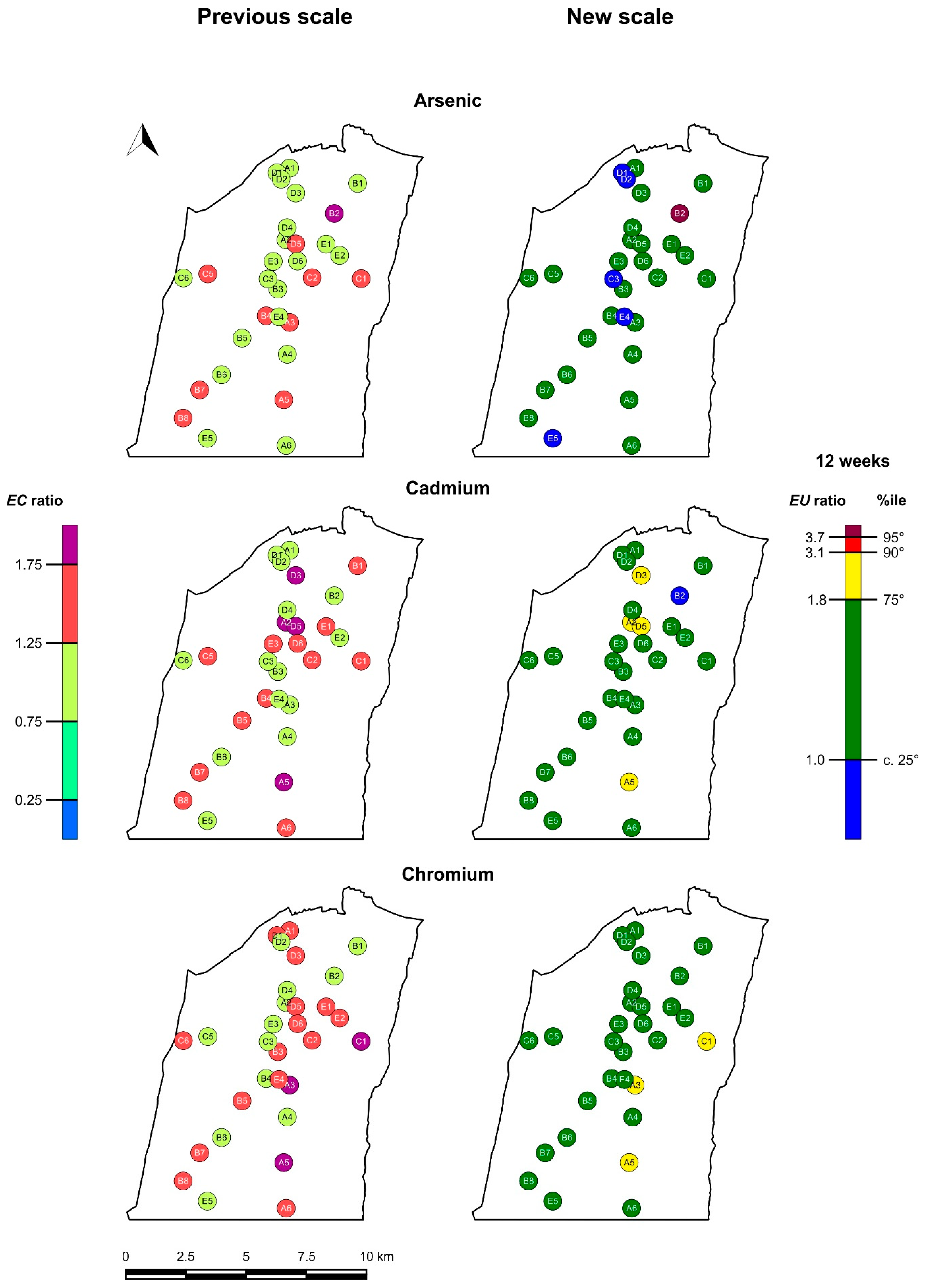
3.2.2. Bioaccumulation Scale for Lichen Transplants
3.3. Comparison between Previous and New Interpretative Scales
4. Conclusions
Supplementary Materials
Author Contributions
Funding
Acknowledgments
Conflicts of Interest
References
- Bargagli, R.; Nimis, P.L.; Monaci, F. Lichen biomonitoring of trace element deposition in urban, industrial and reference areas of Italy. J. Trace Elem. Med. Biol. 1997, 11, 173–175. [Google Scholar] [CrossRef]
- Bargagli, R. Plants as biomonitors of atmospheric pollutants. In Trace Elements in Terrestrial Plants. An Ecophysiological Approach to Biomonitoring and Biorecovering; Springer: Berlin, Germany, 1998; pp. 79–103. [Google Scholar]
- Ferretti, M.; Erhardt, W. Key issues in designing biomonitoring programmes. In Monitoring with Lichens—Monitoring Lichens; Nimis, P.L., Scheidegger, C., Wolseley, P.A., Eds.; Springer: Dordrecht, The Netherlands, 2002; pp. 111–139. [Google Scholar]
- Brunialti, G.; Frati, L. Bioaccumulation with lichens: The Italian experience. Int. J. Environ. Stud. 2014, 71, 15–26. [Google Scholar] [CrossRef]
- Brunialti, G.; Giordani, P.; Ferretti, M. Discriminating between the good and the bad: Quality assurance is central in biomonitoring studies. In Environmental Monitoring; Wiersma, B., Ed.; CRC Press LLC: Boca Raton, FL, USA, 2004; pp. 443–464. [Google Scholar]
- Hays, S.M.; Becker, R.A.; Leung, H.W.; Aylward, L.L.; Pyatt, D.W. Biomonitoring equivalents: A screening approach for interpreting biomonitoring results from a public health risk perspective. Regul. Toxicol. Pharmacol. 2007, 47, 96–109. [Google Scholar] [CrossRef]
- Clewell, H.J.; Tan, Y.M.; Campbell, J.L.; Andersen, M.E. Quantitative interpretation of human biomonitoring data. Toxicol. Appl. Pharmacol. 2008, 231, 122–133. [Google Scholar] [CrossRef] [PubMed]
- Giordano, S.; Adamo, P.; Spagnuolo, V.; Tretiach, M.; Bargagli, R. Accumulation of airborne trace elements in mosses, lichens and synthetic materials exposed at urban monitoring stations: Towards a harmonisation of the moss-bag technique. Chemosphere 2013, 90, 292–299. [Google Scholar] [CrossRef] [PubMed]
- Capozzi, F.; Giordano, S.; Aboal, J.R.; Adamo, P.; Bargagli, R.; Boquete, T.; Di Palma, A.; Real, C.; Reski, R.; Spagnuolo, V.; et al. Best options for the exposure of traditional and innovative moss bags: A systematic evaluation in three European countries. Environ. Pollut. 2016, 214, 362–373. [Google Scholar] [CrossRef] [PubMed]
- Bargagli, R.; Nimis, P.L. Guidelines for the use of epiphytic lichens as biomonitors of atmospheric deposition of trace elements. In Monitoring with Lichens—Monitoring Lichens; Nimis, P.L., Scheidegger, C., Wolseley, P.A., Eds.; Springer: Dordrecht, The Netherlands, 2002; pp. 295–299. [Google Scholar]
- Bennett, J.P. Statistical baseline values for chemical elements in the lichen Hypogymnia physodes. In Environmental Pollution and Plant Responses; Agrawal, S.B., Agrawal, M., Eds.; CRC Press: Boca Raton, FL, USA, 1999; pp. 343–353. [Google Scholar]
- Bargagli, R.; Sanchez-Hernandez, J.C.; Monaci, F. Baseline concentrations of elements in the Antarctic macrolichen Umbilicaria decussata. Chemosphere 1999, 38, 475–487. [Google Scholar] [CrossRef]
- Monaci, F.; Fantozzi, F.; Figueroa, R.; Parra, O.; Bargagli, R. Baseline element composition of foliose and fruticose lichens along the steep climatic gradient of SW Patagonia (Aisén Region, Chile). J. Environ. Monit. 2012, 14, 2309–2316. [Google Scholar] [CrossRef]
- Cecconi, E.; Incerti, G.; Capozzi, F.; Adamo, P.; Bargagli, R.; Benesperi, R.; Candotto Carniel, F.; Favero-Longo, S.E.; Giordano, S.; Puntillo, D.; et al. Background element content of the lichen Pseudevernia furfuracea: A supra-national state of art implemented by novel field data from Italy. Sci. Total Environ. 2018, 622, 282–292. [Google Scholar] [CrossRef] [PubMed]
- Cecconi, E.; Incerti, G.; Capozzi, F.; Adamo, P.; Bargagli, R.; Benesperi, R.; Candotto Carniel, F.; Favero-Longo, S.E.; Giordano, S.; Puntillo, D.; et al. Background element content in the lichen Pseudevernia furfuracea: A comparative analysis of digestion methods. Environ. Monit. Assess. 2019. under review. [Google Scholar]
- Nimis, P.L.; Bargagli, R. Linee-guida per l’utilizzo di licheni epifiti come bioaccumulatori di metalli in traccia. In Atti del Workshop “Biomonitoraggio della Qualità Dell’aria sul Territorio Nazionale”; ANPA Serie Atti; Piccini, C., Salvati, S., Eds.; Roma: Amsterdam, The Netherlands, 1999; pp. 279–289. [Google Scholar]
- Nimis, P.L.; Andreussi, S.; Pittao, E. The performance of two lichen species as bioaccumulators of trace metals. Sci. Total Environ. 2001, 275, 43–51. [Google Scholar] [CrossRef]
- Brunialti, G.; Frati, L. Biomonitoring of nine elements by the lichen Xanthoria parietina in Adriatic Italy: A retrospective study over a 7-year time span. Sci. Total Environ. 2007, 387, 289–300. [Google Scholar] [CrossRef] [PubMed]
- Demiray, A.D.; Yolcubal, I.; Akyol, N.H.; Çobanoğlu, G. Biomonitoring of airborne metals using the Lichen Xanthoria parietina in Kocaeli Province, Turkey. Ecol. Ind. 2012, 18, 632–643. [Google Scholar] [CrossRef]
- Pirintsos, S.; Bariotakis, M.; Kalogrias, V.; Katsogianni, S.; Brüggemann, R. Hasse diagram technique can further improve the interpretation of results in multielemental large-scale biomonitoring studies of atmospheric metal pollution. In Multi-Indicator Systems and Modelling in Partial Order; Brüggemann, R., Carlsen, L., Wittmann, J., Eds.; Springer: New York, NY, USA, 2014; pp. 237–251. [Google Scholar]
- Cocozza, C.; Ravera, S.; Cherubini, P.; Lombardi, F.; Marchetti, M.; Tognetti, R. Integrated biomonitoring of airborne pollutants over space and time using tree rings, bark, leaves and epiphytic lichens. Urban For. Urban Green. 2016, 17, 177–191. [Google Scholar] [CrossRef]
- Paoli, L.; Winkler, A.; Guttová, A.; Sagnotti, L.; Grassi, A.; Lackovičová, A.; Senko, D.; Loppi, S. Magnetic properties and element concentrations in lichens exposed to airborne pollutants released during cement production. Environ. Sci. Pollut. Res. 2017, 24, 12063–12080. [Google Scholar] [CrossRef] [PubMed]
- Lucadamo, L.; Corapi, A.; Gallo, L. Evaluation of glyphosate drift and anthropogenic atmospheric trace elements contamination by means of lichen transplants in a southern Italian agricultural district. Air Qual. Atmos. Health 2018, 11, 325–339. [Google Scholar] [CrossRef]
- Tretiach, M.; Baruffo, L. Contenuto di elementi in traccia in talli di Parmelia borreri e Xanthoria parietina raccolti sullo stesso forofita. Not. Soc. Lich. Ital. 2001, 14, 70. [Google Scholar]
- Minganti, V.; Capelli, R.; Drava, G.; De Pellegrini, R.; Brunialti, G.; Giordani, P.; Modenesi, P. Biomonitoring of trace metals by different species of lichens (Parmelia) in north-west Italy. J. Atmos. Chem. 2003, 45, 219–229. [Google Scholar] [CrossRef]
- Bergamaschi, L.; Rizzio, E.; Giaveri, G.; Loppi, S.; Gallorini, M. Comparison between the accumulation capacity of four lichen species transplanted to a urban site. Environ. Pollut. 2007, 148, 468–476. [Google Scholar] [CrossRef]
- Frati, L.; Brunialti, G.; Loppi, S. Problems related to lichen transplants to monitor trace element deposition in repeated surveys: A case study from central Italy. J. Atmos. Chem. 2005, 52, 221–230. [Google Scholar] [CrossRef]
- Loppi, S.; Giordani, P.; Brunialti, G.; Isocrono, D.; Piervittori, R. A new scale for the interpretation of lichen biodiversity values in the Thyrrenian side of Italy. Bibl. Lichenol. 2002, 82, 235–242. [Google Scholar]
- Baffi, C.; Bettinelli, M.; Beone, G.M.; Spezia, S. Comparison of different analytical procedures in the determination of trace elements in lichens. Chemosphere 2002, 48, 299–306. [Google Scholar] [CrossRef]
- Yafa, C.; Farmer, J.G. A comparative study of acid-extractable and total digestion methods for the determination of inorganic elements in peat material by inductively coupled plasma-optical emission spectrometry. Anal. Chim. Acta 2006, 557, 296–303. [Google Scholar] [CrossRef]
- Tam, N.F.Y.; Yao, M.W.Y. Three digestion methods to determine concentrations of Cu, Zn, Cd, Ni, Pb, Cr, Mn, and Fe in mangrove sediments from Sai Keng, Chek Keng, and Sha Tau Kok, Hong Kong. Bull. Environ. Contam. Toxicol. 1999, 62, 708–716. [Google Scholar] [CrossRef]
- Fortuna, L.; Tretiach, M. Effects of site-specific climatic conditions on the radial growth of the lichen biomonitor Xanthoria parietina. Environ. Sci. Pollut. Res. 2018, 25, 34017–34026. [Google Scholar] [CrossRef] [PubMed]
- Gaudet, C.L.; Bright, D.; Adare, K.; Potter, K. A rank-based approach to deriving Canadian soil and sediment: Quality guidelines. In Species Sensitivity Distributions in Ecotoxicology, 1st ed.; Posthuma, L., Suter, G.W., II, Traas, T.P., Eds.; CRC Press: Boca Raton, FL, USA, 2001; pp. 255–273. [Google Scholar]
- Reimann, C.; Garrett, R.G. Geochemical background—Concept and reality. Sci. Total Environ. 2005, 350, 12–27. [Google Scholar] [CrossRef] [PubMed]
- Facchinelli, A.; Sacchi, E.; Mallen, L. Multivariate statistical and GIS-based approach to identify heavy metal sources in soils. Environ. Pollut. 2001, 114, 313–324. [Google Scholar] [CrossRef]
- Massas, I.; Ehliotis, C.; Gerontidis, S.; Sarris, E. Elevated heavy metal concentrations in top soils of an Aegean island town (Greece): Total and available forms, origin and distribution. Environ. Monit. Assess. 2009, 151, 105–116. [Google Scholar] [CrossRef]
- Yang, C.L.; Wu, Z.F.; Zhang, H.H.; Guo, R.P.; Wu, Y.Q. Risk assessment and distribution of soil Pb in Guandong, China. Environ. Monit. Assess. 2009, 159, 381–391. [Google Scholar] [CrossRef]
- Reimann, C.; de Caritat, P. Establishing geochemical background variation and threshold values for 59 elements in Australian surface soil. Sci. Total Environ. 2017, 578, 633–648. [Google Scholar] [CrossRef]
- Hoaglin, D.C.; Iglewicz, B.; Tukey, J.W. Performance of some resistant rules for outlier labeling. J. Am. Stat. Assoc. 1986, 81, 991–999. [Google Scholar] [CrossRef]
- Cicchitelli, G.; Herzel, A.; Montanari, G.E. Il Campionamento Statistico, 2nd ed.; Il Mulino: Bologna, Italy, 1992. [Google Scholar]
- ARPA FVG. Available online: http://www.arpa.fvg.it/cms/hp/news/Studio-licheni-centrale-a2a.html (accessed on 19 February 2019).
- Fortuna, L. Development of Biomonitoring Techniques of Persistent Airborne Pollutants Using Native Lichens. Ph.D. Thesis, University of Trieste, Trieste, Italy, 27 March 2018. [Google Scholar]
- EU Directive 2008/50/EC. Available online: https://eur-lex.europa.eu/legal-content/EN/TXT/PDF/?uri=CELEX: 32008L0050&from=en (accessed on 19 February 2019).
- IARC. 2018. Available online: https://monographs.iarc.fr/wp-content/uploads/2018/06/mono100C-9.pdf (accessed on 19 February 2019).
- Tretiach, M.; Candotto Carniel, F.C.; Loppi, S.; Carniel, A.; Bortolussi, A.; Mazzilis, D.; Del Bianco, C. Lichen transplants as a suitable tool to identify mercury pollution from waste incinerators: A case study from NE Italy. Environ. Monit. Assess. 2011, 175, 589–600. [Google Scholar] [CrossRef] [PubMed]
- Nimis, P.L. The Lichens of Italy. A Second Annotated Catalogue; EUT: Trieste, Italy, 2016. [Google Scholar]
- Incerti, G.; Cecconi, E.; Capozzi, F.; Adamo, P.; Bargagli, R.; Benesperi, R.; Candotto Carniel, F.; Cristofolini, F.; Giordano, S.; Puntillo, D.; et al. Infraspecific variability in baseline element composition of the epiphytic lichen Pseudevernia furfuracea in remote areas: Implications for biomonitoring of air pollution. Environ. Sci. Pollut. Res. 2017, 24, 8004–8016. [Google Scholar] [CrossRef] [PubMed]
- Weltje, L.; Sumpter, J.P. What makes a concentration environmentally relevant? Critique and a proposal. Environ. Sci. Technol. 2017, 51, 11520–11521. [Google Scholar] [CrossRef] [PubMed]
- Wolterbeek, H.T.; Bode, P. Strategies in sampling and sample handling in the context of large-scale plant biomonitoring surveys of trace element air pollution. Sci. Total Environ. 1995, 176, 33–43. [Google Scholar] [CrossRef]
- Nieboer, E.; Richardson, D.H.S.; Tomassini, F.D. Mineral uptake and release by lichens: An overview. Bryologist 1978, 81, 226–246. [Google Scholar] [CrossRef]
- Nash, T.H., III. Nutrients, elemental accumulation, mineral cycling. In Lichen Biology, 2nd ed.; Nash, T.H., III, Ed.; Cambridge University Press: Cambridge, UK, 2008; pp. 236–253. [Google Scholar]
- Brown, D.H.; Beckett, R.P. Uptake and effect of cations on lichen metabolism. Lichenologist 1984, 16, 173–188. [Google Scholar] [CrossRef]
- Paoli, L.; Vannini, A.; Fačkovcová, Z.; Guarnieri, M.; Bačkor, M.; Loppi, S. One year of transplant: Is it enough for lichens to reflect the new atmospheric conditions? Ecol. Ind. 2018, 88, 495–502. [Google Scholar] [CrossRef]
- Mikhailova, I. Transplanted lichens for bioaccumulation studies. In Monitoring with Lichens—Monitoring Lichens; Nimis, P.L., Scheidegger, C., Wolseley, P.A., Eds.; Springer: Dordrecht, The Netherlands, 2002; pp. 301–304. [Google Scholar]
- Gailey, F.A.Y.; Lloyd, O.L. Methodological investigations into low technology monitoring of atmospheric metal pollution: Part 2—The effects of length of exposure on metal concentrations. Environ. Pollut. B 1986, 12, 61–74. [Google Scholar] [CrossRef]
- Bargagli, R.; Mikhailova, I. Accumulation of inorganic contaminants. In Monitoring with Lichens—Monitoring Lichens; Nimis, P.L., Scheidegger, C., Wolseley, P.A., Eds.; Springer: Dordrecht, The Netherlands, 2002; pp. 65–84. [Google Scholar]
- Zhang, J.; Zhao, Y.; Ding, F.; Zeng, H.; Zheng, C. Preliminary study of trace element emissions and control during coal combustion. Front. Energ. Power Eng. China 2007, 1, 273–279. [Google Scholar] [CrossRef]
- Wang, C.; Liu, H.; Zhang, Y.; Zou, C.; Anthony, E.J. Review of arsenic behavior during coal combustion: Volatilization, transformation, emission and removal technologies. Prog. Energy Comb. Sci. 2018, 68, 1–28. [Google Scholar] [CrossRef]
- ARIANET. Available online: http://www.a2aenergiefuture.eu/gruppo/export/sites/default/ene/impianti/documenti_impianti/ARIANET-R2014.23-MONFALCONE.pdf (accessed on 19 February 2019).
- Wilson, N.; Horrocks, J. Lessons from the removal of lead from gasoline for controlling other environmental pollutants: A case study from New Zealand. Environ. Health 2008, 7, 1. [Google Scholar] [CrossRef] [PubMed]
- Madsen, C.; Gehring, U.; Håberg, S.E.; Nafstad, P.; Meliefste, K.; Nystad, W.; Lødrup Carlsen, K.C.; Brunekreef, B. Comparison of land-use regression models for predicting spatial NOx contrasts over a three year period in Oslo, Norway. Atmos. Environ. 2011, 45, 3576–3583. [Google Scholar] [CrossRef]
- Kollanus, V.; Tiittanen, P.; Niemi, J.V.; Lanki, T. Effects of long-range transported air pollution from vegetation fires on daily mortality and hospital admissions in the Helsinki metropolitan area, Finland. Environ. Res. 2016, 151, 351–358. [Google Scholar] [CrossRef] [PubMed]
- Gotelli, N.J.; Ellison, A.M. A Primer of Ecological Statistics, 2nd ed.; Sinauer Associates: Sunderland, MA, USA, 2012. [Google Scholar]


| Glossary | |
|---|---|
| Native lichens | Lichens grown in a target study area. |
| Background element concentration values (BECs) | Species-specific element concentration values measured in lichen samples reflecting proximate-natural, unaltered conditions. |
| Bioaccumulation ratio (B ratio) | The dimensionless ratio between species-specific element concentration values measured in native samples and the corresponding background values. |
| Lichen transplants | Lichens collected in a proximate-natural site and afterwards transplanted for a certain exposure time span to a target study area. |
| Exposed samples | In the context of lichen transplants, samples transplanted to a target study area, exposed to pollutant depositions for a certain exposure time span, and then subjected to the determination of elemental concentration. |
| Unexposed samples | In the context of lichen transplants, samples collected in a proximate-natural site and subjected to the determination of elemental concentration. These samples are used as a benchmark to assess the magnitude of lichen bioaccumulation after transplantation. |
| Exposed-to-unexposed ratio (EU ratio) | The dimensionless ratio between species-specific element concentration values measured in exposed samples and the corresponding element concentration values measured in unexposed samples. |
| Exposed-to-control ratio (EC ratio) | Previous name of the EU ratio [27], here terminologically revised. |
| Element | Flavoparmelia caperata | Xanthoria parietina | ||||||||||||
|---|---|---|---|---|---|---|---|---|---|---|---|---|---|---|
| n | Mean | Med | Range | IQR | S | K | n | Mean | Med | Range | IQR | S | K | |
| Al | 244 | 551 | 348 | 110–4224 | 252–526 | 3.24 | 11.63 | 68 | 656 | 605 | 150–3408 | 371–722 | 3.58 | 16.28 |
| As | 367 | 0.34 | 0.25 | 0.06–1.90 | 0.18–0.40 | 2.63 | 9.08 | 79 | 0.35 | 0.28 | 0.06–2.31 | 0.15–0.40 | 3.41 | 14.59 |
| Cd | 298 | 0.30 | 0.25 | 0.06–1.69 | 0.18–0.37 | 2.62 | 13.68 | 80 | 0.15 | 0.09 | 0.04–1.46 | 0.07–0.15 | 4.73 | 27.97 |
| Cr | 321 | 2.44 | 1.84 | 0.35–24.94 | 1.17–2.66 | 4.80 | 33.16 | 77 | 2.39 | 1.91 | 0.69–10.52 | 1.61–2.73 | 2.82 | 10.87 |
| Cu | 321 | 8.58 | 7.38 | 2.50–78.29 | 6.23–9.34 | 6.99 | 67.44 | 98 | 5.83 | 5.48 | 3.20–19.27 | 4.45–6.31 | 3.17 | 13.29 |
| Hg | 182 | 0.09 | 0.08 | 0.01–0.43 | 0.06–0.11 | 1.91 | 8.97 | 77 | 0.06 | 0.05 | 0.01–0.63 | 0.04–0.07 | 5.55 | 37.18 |
| Ni | 296 | 3.14 | 2.67 | 0.32–19.01 | 1.27–4.03 | 2.61 | 9.42 | 51 | 3.39 | 2.66 | 0.82–11.2 | 1.55–4.68 | 1.45 | 2.68 |
| Pb | 321 | 6.0 | 4.0 | 0.8–114.2 | 2.40–6.30 | 7.24 | 69.56 | 98 | 2.37 | 1.64 | 0.36–15.40 | 1.00–2.67 | 3.03 | 11.78 |
| Ti | 184 | 41.8 | 26.4 | 0.3–309.0 | 19.4–40.7 | 2.80 | 9.21 | 42 | 59.8 | 48.9 | 15.2–262.0 | 37.2–60.0 | 3.00 | 10.57 |
| V | 150 | 1.71 | 0.94 | 0.34–13.22 | 0.75–1.60 | 2.87 | 10.67 | n.a. | n.a. | n.a. | n.a. | n.a. | n.a. | |
| Zn | 321 | 47.3 | 44.0 | 17.7–330.8 | 35.3–53.0 | 6.17 | 65.08 | 98 | 30.0 | 25.6 | 13.0–168.0 | 21.2–34.4 | 4.88 | 33.51 |
| Element | Flavoparmelia caperata | Xanthoria parietina | Mann–Whitney U Test | ||||||||
|---|---|---|---|---|---|---|---|---|---|---|---|
| BEC | BEC Dataset | BEC | BEC Dataset | ||||||||
| n | Mean ± SD | Med ± MAD | n | Mean ± SD | Med ± MAD | U | Z | p-Value | |||
| Al | 253 | 61 | 201 ± 37 | 209 ± 26 | 372 | 17 | 295 ± 59 | 300 ± 34 | 87.5 | −5.215 | 1.8 × 10⁻⁷ |
| As | 0.18 | 91 | 0.14 ± 0.03 | 0.15 ± 0.02 | 0.15 | 19 | 0.11 ± 0.02 | 0.11 ± 0.01 | 329.0 | 4.238 | 2.3 × 10⁻⁵ |
| Cd | 0.18 | 68 | 0.14 ± 0.03 | 0.13 ± 0.02 | 0.07 | 19 | 0.05 ± 0.01 | 0.05 ± 0.01 | 13.0 | 6.505 | 7.8 × 10⁻¹¹ |
| Cr | 1.17 | 80 | 0.85 ± 0.24 | 0.90 ± 0.20 | 1.61 | 19 | 1.20 ± 0.28 | 1.10 ± 0.20 | 293.0 | −4.149 | 3.3 × 10⁻⁵ |
| Cu | 6.2 | 80 | 5.2 ± 0.9 | 5.5 ± 0.5 | 4.5 | 25 | 4.1 ± 0.3 | 4.1 ± 0.2 | 221.0 | 5.859 | 4.7 × 10⁻⁹ |
| Hg | 0.057 | 45 | 0.031 ± 0.021 | 0.038 ± 0.019 | 0.035 | 18 | 0.019 ± 0.009 | 0.021 ± 0.008 | 328.0 | 1.308 | 0.191 |
| Ni | 1.27 | 73 | 0.91 ± 0.20 | 0.93 ± 0.17 | 1.64 | 13 | 1.28 ± 0.22 | 1.33 ± 0.16 | 108.5 | −4.408 | 1.0 × 10⁻⁵ |
| Pb | 2.37 | 80 | 1.71 ± 0.45 | 1.82 ± 0.48 | 1.00 | 24 | 0.67 ± 0.21 | 0.70 ± 0.21 | 21.0 | 7.243 | 4.4 × 10⁻¹³ |
| Ti | 19.5 | 46 | 12.8 ± 5.8 | 14.8 ± 4.3 | 37.3 | 11 | 29.3 ± 7.3 | 31.6 ± 4.2 | 22.5 | −4.652 | 3.3 × 10⁻⁶ |
| V | 0.75 | 37 | 0.61 ± 0.11 | 0.62 ± 0.07 | n.a. | n.a. | n.a. | n.a. | n.a. | n.a. | n.a. |
| Zn | 35.3 | 80 | 29.6 ± 4.3 | 30.1 ± 3.2 | 21.3 | 25 | 17.9 ± 2.6 | 19.0 ± 1.9 | 30.0 | 7.296 | 3.0 × 10⁻¹³ |
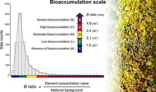
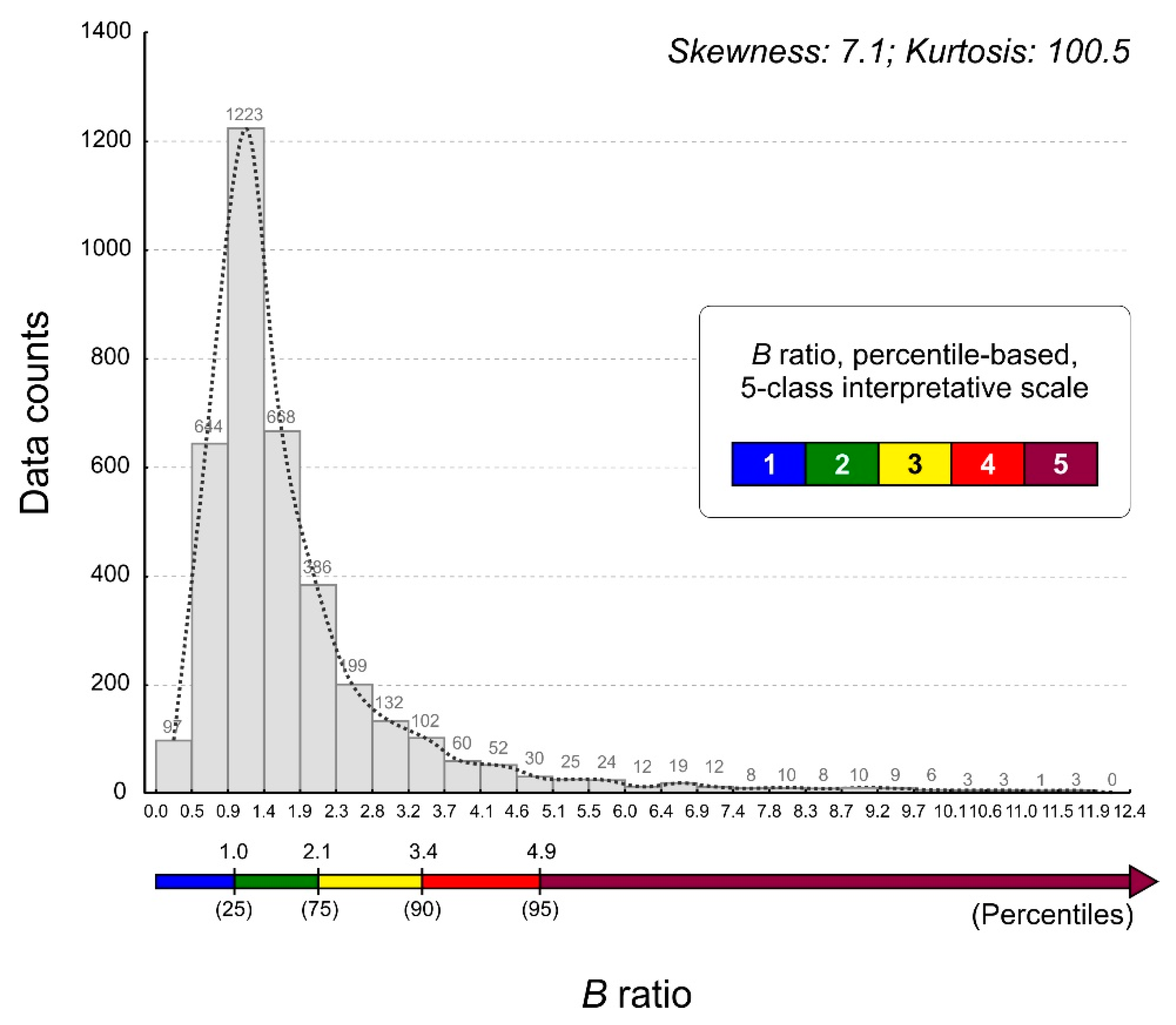
| Bioaccumulation Class | Percentile Thresholds | B Ratio | Color Code | |||||
|---|---|---|---|---|---|---|---|---|
| ID | Description (Abbreviation) | RGB | HTML | |||||
| 1 | Absence of bioaccumulation | (A) | ≤25th | ≤1.0 | 0 | 0 | 255 | #0000FF |
| 2 | Low bioaccumulation | (L) | (25th, 75th] | (1.0, 2.1] | 0 | 128 | 0 | #008000 |
| 3 | Moderate bioaccumulation | (M) | (75th, 90th] | (2.1, 3.4] | 255 | 243 | 15 | #FFF30F |
| 4 | High bioaccumulation | (H) | (90th, 95th] | (3.4, 4.9] | 255 | 0 | 0 | #FF0000 |
| 5 | Severe bioaccumulation | (S) | >95th | >4.9 | 128 | 0 | 64 | #800040 |
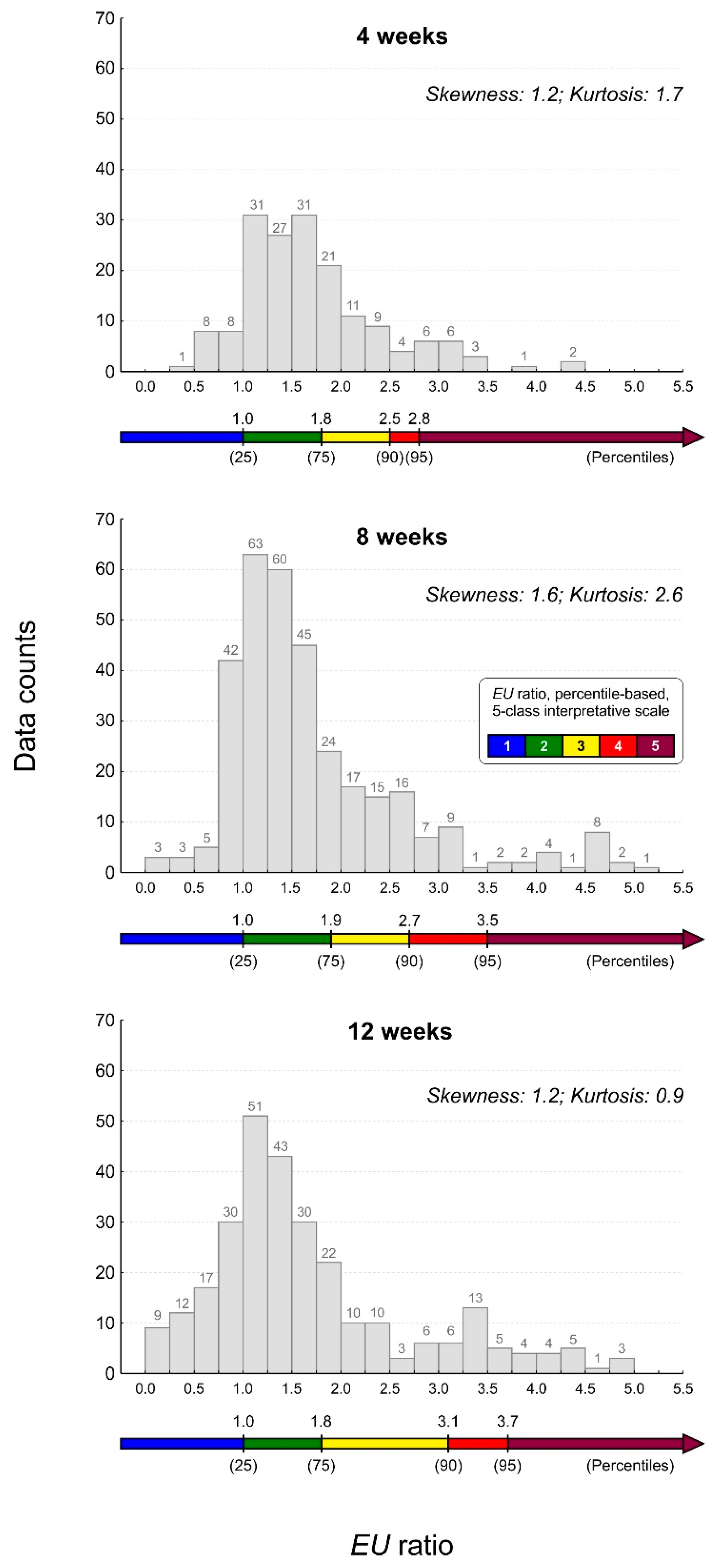
| Bioaccumulation Class | Percentile Thresholds | EU Ratio | Color Code | |||||||
|---|---|---|---|---|---|---|---|---|---|---|
| ID | Description (Abbreviation) | 4 Weeks | 8 Weeks | 12 Weeks | RGB | HTML | ||||
| 1 | Absence of bioaccumulation | (A) | ≤25th * | ≤1.0 | ≤1.0 | ≤1.0 | 0 | 0 | 255 | #0000FF |
| 2 | Low bioaccumulation | (L) | (25th, 75th] | (1.0, 1.8] | (1.0, 1.9] | (1.0, 1.8] | 0 | 128 | 0 | #008000 |
| 3 | Moderate bioaccumulation | (M) | (75th, 90th] | (1.8, 2.5] | (1.9, 2.7] | (1.8, 3.1] | 255 | 243 | 15 | #FFF30F |
| 4 | High bioaccumulation | (H) | (90th, 95th] | (2.5, 2.8] | (2.7, 3.5] | (3.1, 3.7] | 255 | 0 | 0 | #FF0000 |
| 5 | Severe bioaccumulation | (S) | >95th | >2.8 | >3.5 | >3.7 | 128 | 0 | 64 | #800040 |
© 2019 by the authors. Licensee MDPI, Basel, Switzerland. This article is an open access article distributed under the terms and conditions of the Creative Commons Attribution (CC BY) license (http://creativecommons.org/licenses/by/4.0/).
Share and Cite
Cecconi, E.; Fortuna, L.; Benesperi, R.; Bianchi, E.; Brunialti, G.; Contardo, T.; Di Nuzzo, L.; Frati, L.; Monaci, F.; Munzi, S.; et al. New Interpretative Scales for Lichen Bioaccumulation Data: The Italian Proposal. Atmosphere 2019, 10, 136. https://doi.org/10.3390/atmos10030136
Cecconi E, Fortuna L, Benesperi R, Bianchi E, Brunialti G, Contardo T, Di Nuzzo L, Frati L, Monaci F, Munzi S, et al. New Interpretative Scales for Lichen Bioaccumulation Data: The Italian Proposal. Atmosphere. 2019; 10(3):136. https://doi.org/10.3390/atmos10030136
Chicago/Turabian StyleCecconi, Elva, Lorenzo Fortuna, Renato Benesperi, Elisabetta Bianchi, Giorgio Brunialti, Tania Contardo, Luca Di Nuzzo, Luisa Frati, Fabrizio Monaci, Silvana Munzi, and et al. 2019. "New Interpretative Scales for Lichen Bioaccumulation Data: The Italian Proposal" Atmosphere 10, no. 3: 136. https://doi.org/10.3390/atmos10030136
APA StyleCecconi, E., Fortuna, L., Benesperi, R., Bianchi, E., Brunialti, G., Contardo, T., Di Nuzzo, L., Frati, L., Monaci, F., Munzi, S., Nascimbene, J., Paoli, L., Ravera, S., Vannini, A., Giordani, P., Loppi, S., & Tretiach, M. (2019). New Interpretative Scales for Lichen Bioaccumulation Data: The Italian Proposal. Atmosphere, 10(3), 136. https://doi.org/10.3390/atmos10030136