Assessing the Performance of CMIP5 GCMs for Projection of Future Temperature Change over the Lower Mekong Basin


Abstract
1. Introduction
2. Data and Methods
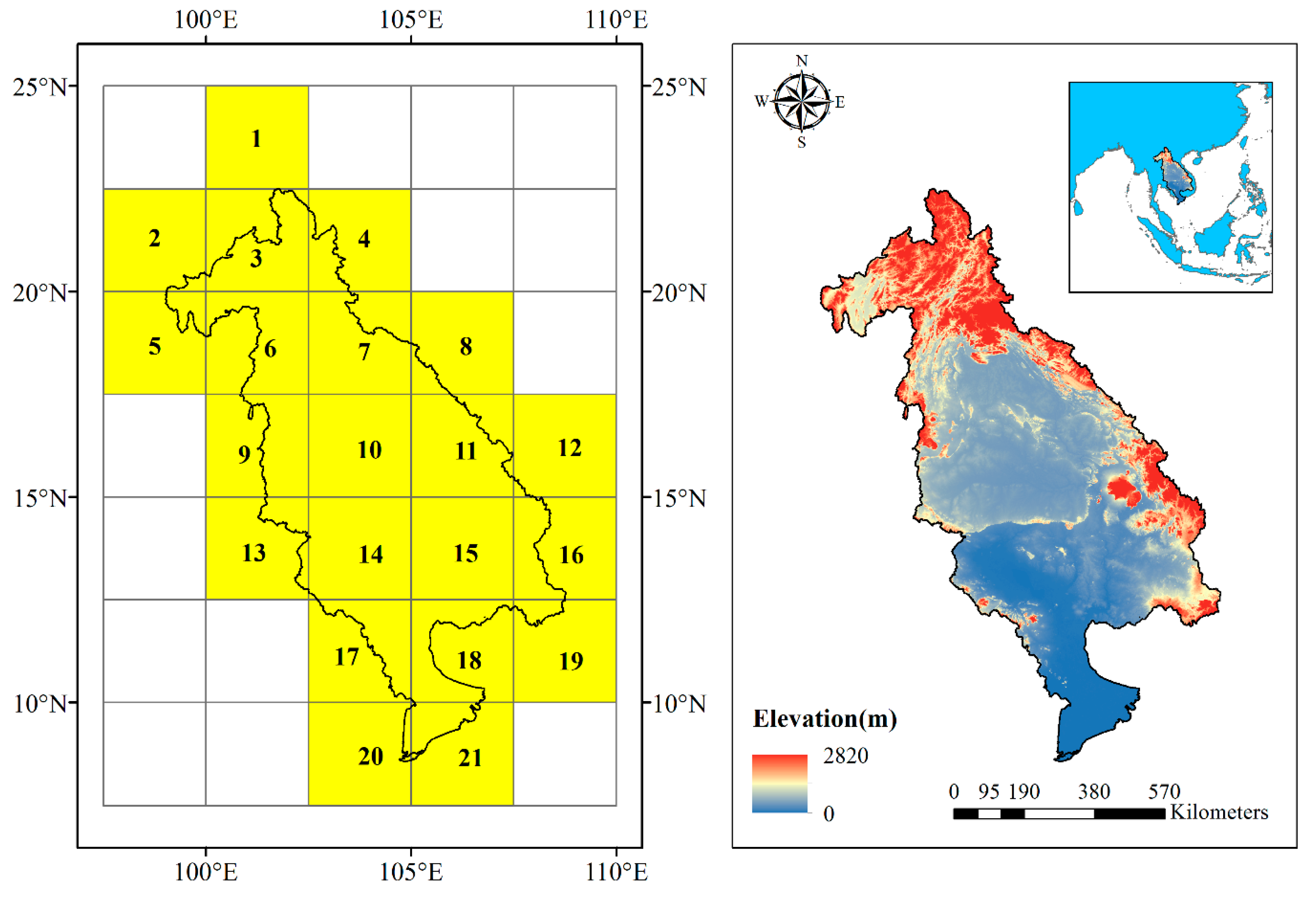
2.1. Data
2.1.1. GCM Data
2.1.2. Temperature Data
2.2. Methods
2.2.1. Assessment of the Performance for CMIP5 GCMs
- Mean valueThe mean value (M) is defined as follows:Here Ti represents the monthly temperature for the LMB at ith time step, and n represents the total number of the time steps.
- Standard deviationThe standard deviation (SD) is defined as follows:Here Ti represents the monthly temperature for the LMB at ith time step, represents the mean monthly temperature for the LMB, and n represents the total number of the time steps. A smaller value of SD indicates a better performance of a GCM.
- Normalized root mean square errorThe normalized root mean square error (NRMSE) is defined as follows:Here Tmi and Toi represent the monthly temperature for the GCM and the observed value for the LMB at ith time step, respectively. represents the mean value of the observed value for the LMB. n represents the total number of the time steps. A smaller value of NRMSE indicates a better performance of a GCM.
- Linear correlation coefficient (r) for spatial distributionThe correlation coefficient (r) was used to as a measure to compare spatial distribution of temperature between the observation and the GCMs. The sample size is 21, and r was calculated between the observation and the GCMs for long-term mean values of each grid. The formula is defined as follows:Tmi and Toi represent temperature for the GCM and the observation of the mean annual values at ith grid, respectively, and the and represent the corresponding mean values for temperature of the GCM and the observation of all grids, respectively. A larger value of the r indicates a better performance of a GCM.
- Mann‒Kendall test statistic Z and Sen’s slopeThe Mann‒Kendall test statistic Z and Sen’s slope were used to obtain the trends and their magnitudes for GCMs and observations. Thus, the ability of how well the GCMs represent the variation trend of the observations can be obtained. The statistics of the annual time series were used for analysis.Here xk, xi are the sequential temperature values, n is the length (44) of the dataset, andandHere t is the extent of any given tie and ∑ denotes the summation over all ties.Here 1 < j < i < n, and the slope estimator β represents the median of the entire dataset.
- Probability density functions (PDF)The Significance score (Sscore) was used to assess the GCM’s probability density functions (PDF) for monthly temperature. The formula is defined as follows [46]:Here Bmi and Boi represent the probability of GCM and observed temperature values at the ith of bin, respectively.
- Improved RS (Rank Score)The improved RS distinguishes between the relative error index and non-relative error index in comparison to the RS method, which could avoid inconsistent results [40]. For example, a smaller value of NRMSE of the relative error index indicates a better performance of a GCM, while a larger value of r of the non-error index indicates a better performance of a GCM. Thus, the improved RS can be used for different assessment criteria and climatic variables to comprehensively assess the performance of GCMs in the regions. The Rank Score of each assessment criterion can be calculated by its statistic [40]:Here RSi represents the score for GCM calculated by an assessment criterion i. For the relative error indexes of M, SD, Z and Sen’s slope, Ti represents absolute error that was calculated between a GCM and the observation (Equation (12)), and Tmin and Tmax represent the corresponding minimum and maximum among all GCMs. Moreover, for the relative error indexes of NRMSE, Ti represents the absolute value of statistic for a GCM, and Tmin and Tmax represent the corresponding minimum and maximum among all GCMs. For the non-relative error index of r and Sscore, Ti represents the absolute value of the statistic for a GCM, and Tmin and Tmax represent the corresponding minimum and maximum among all GCMs.Here Tsm and Tso represent the statistics of the GCM and the observation, respectively.Therefore, the overall RS for temperature can be calculated as follows:Here RST represents the overall RS of temperature for the GCM. Here n = 7 and i represents an assessment criterion, such as M, SD, NRMSE, Z, Sen’s slope, spatial distribution r, and Sscore. Wi represents the weight for an assessment criterion i, Ws represents the sum weight of all the assessment criteria. Since Z and Sen’s slope are part of trend analysis, we set 0.5 weight for Z, Sen’s slope, respectively, while 1.0 weight for M, SD, NRMSE, r, and Sscore, respectively.
2.2.2. Projection of Future Temperature Change
3. Results
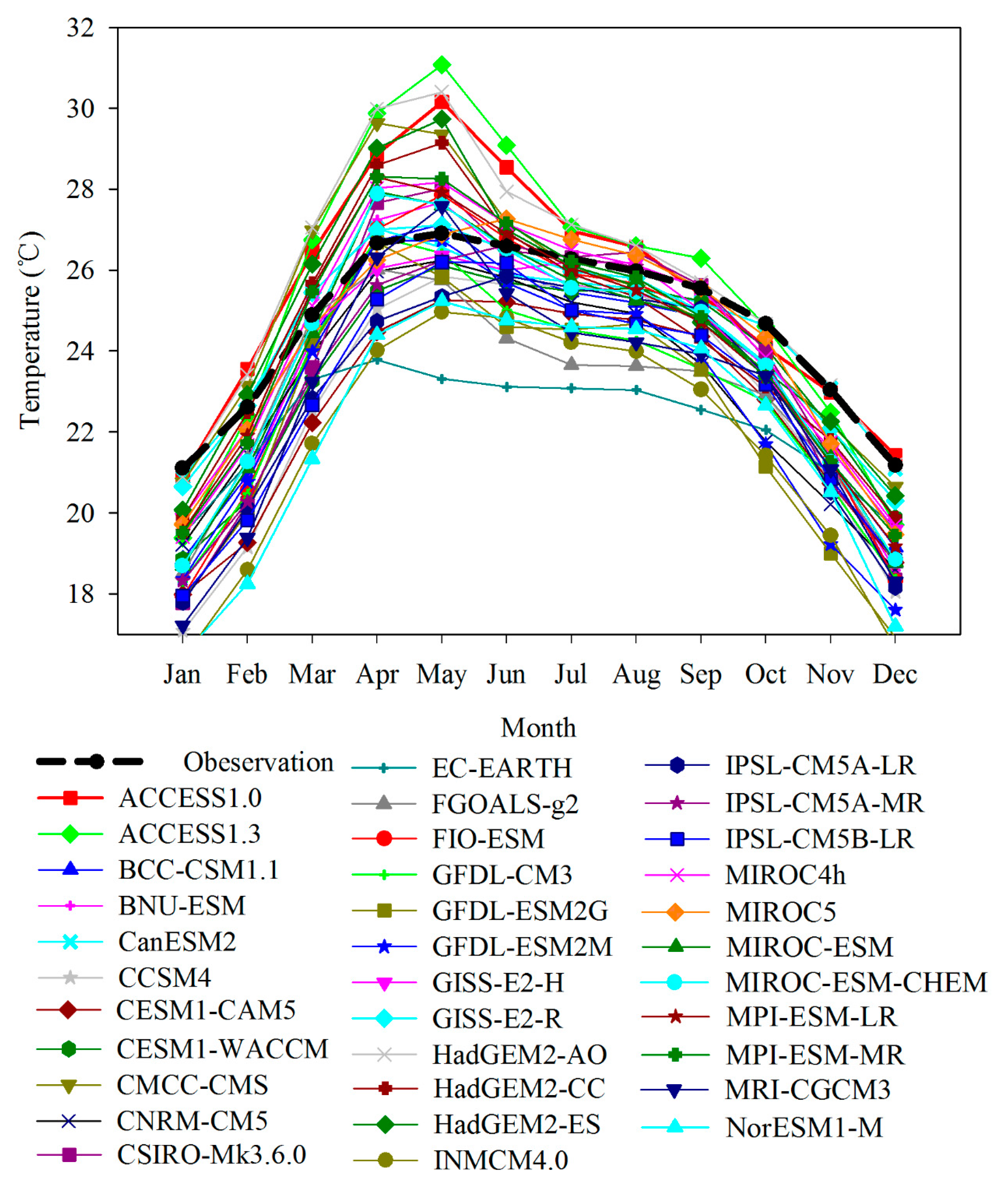
3.1. Annual Cycle of Temperature
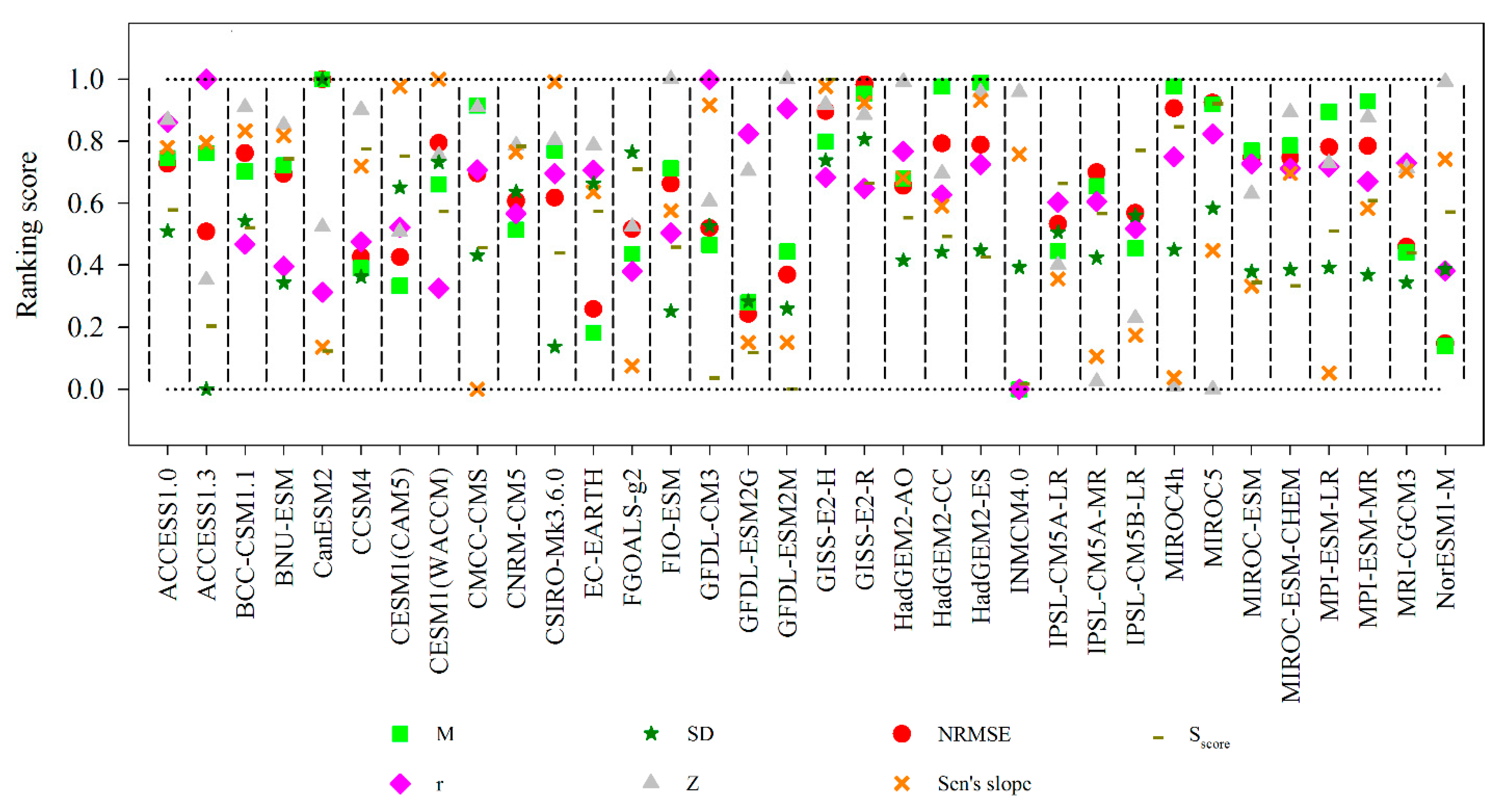
3.2. Characteristics of Statistics in Criteria
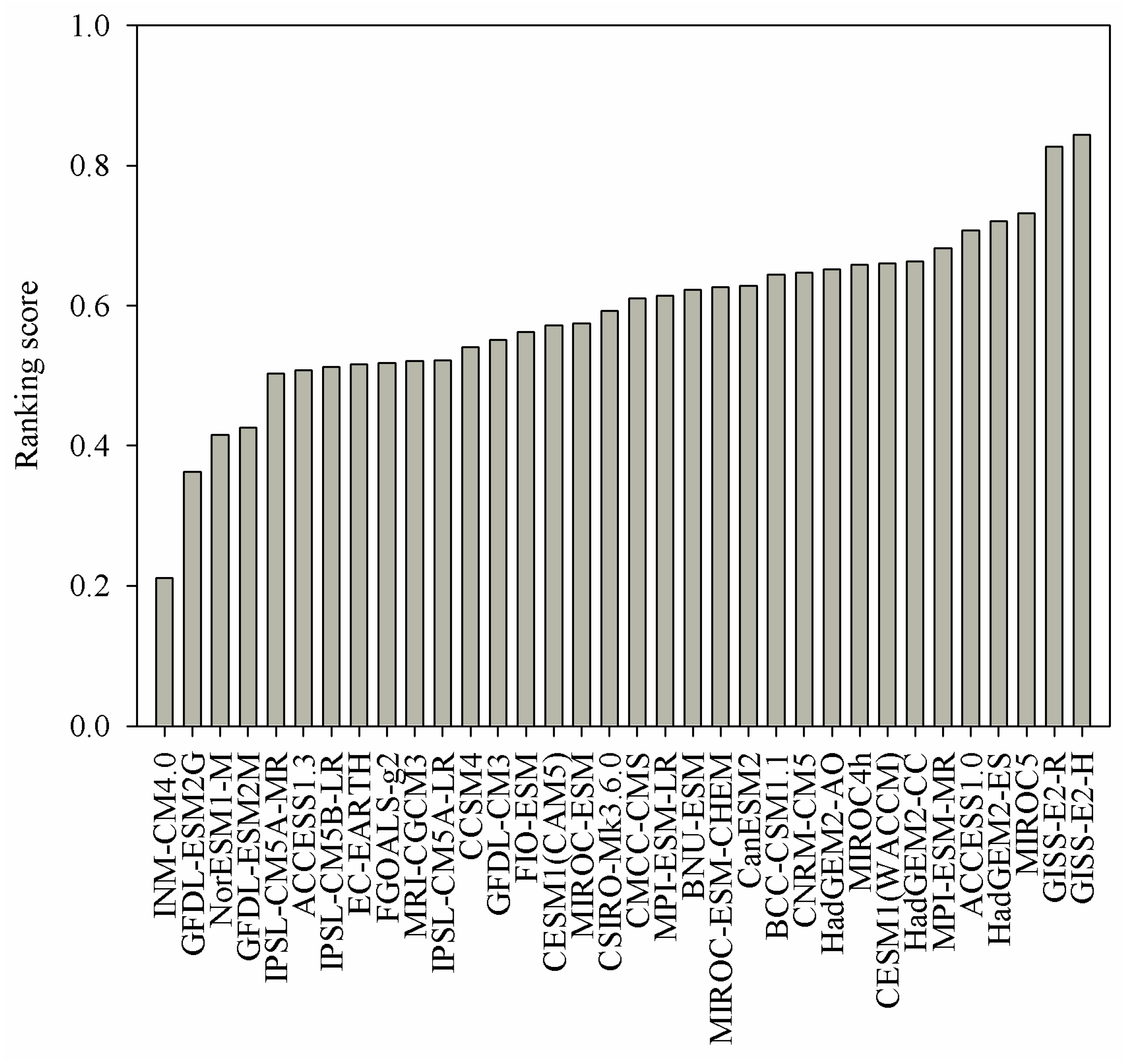
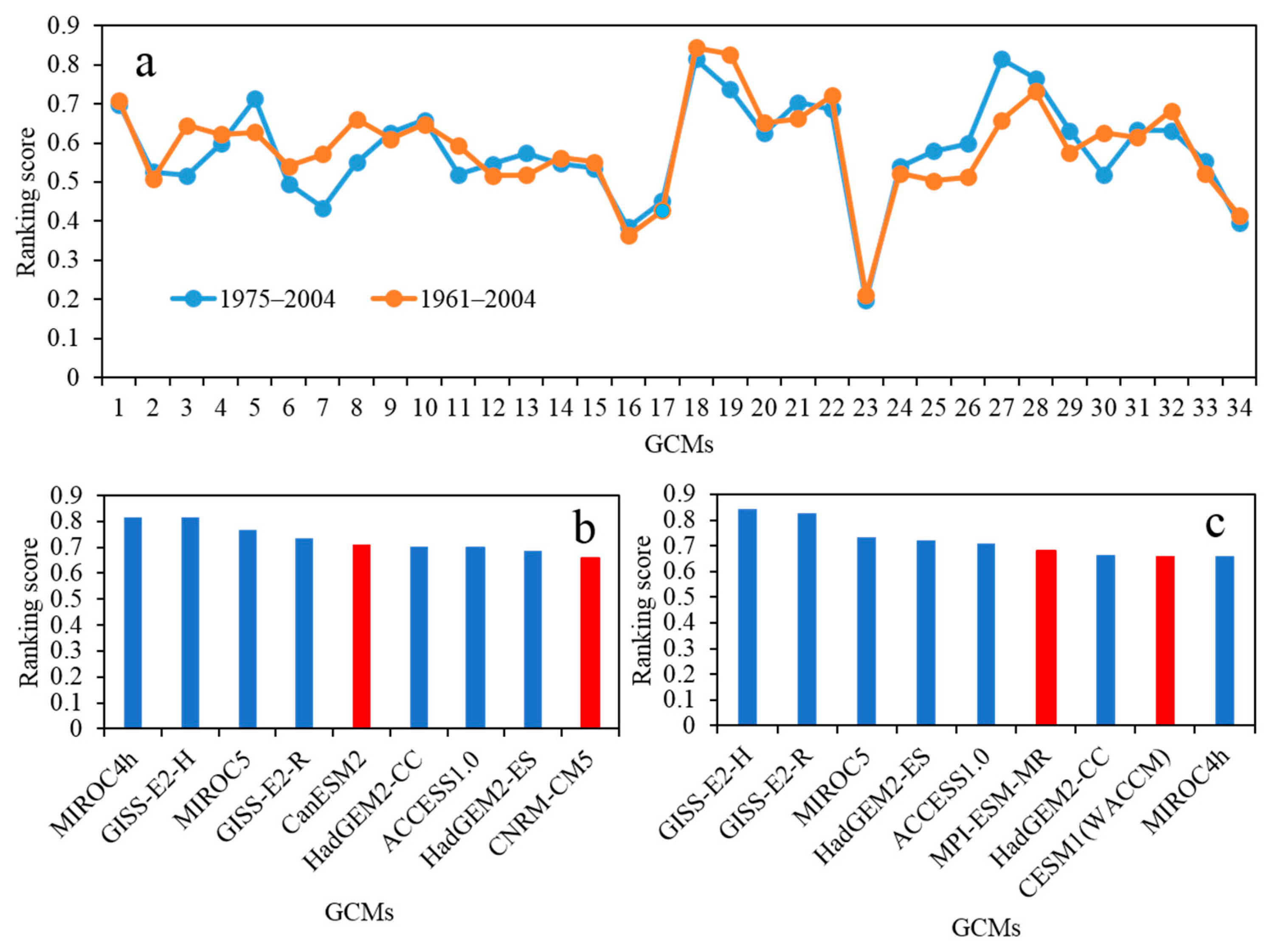
3.3. Comparison of the Performance of the GCMs
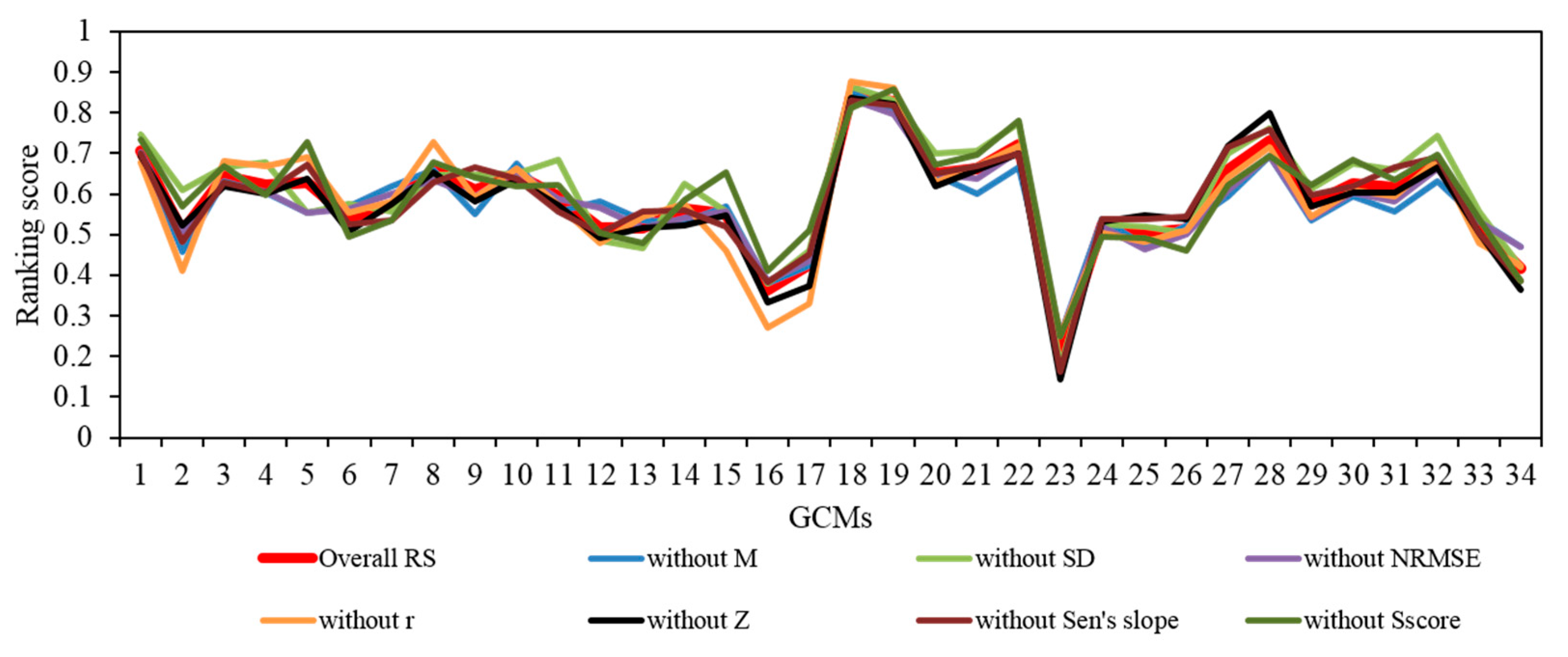
3.4. Sensitivity Analysis of the GCMs Performance
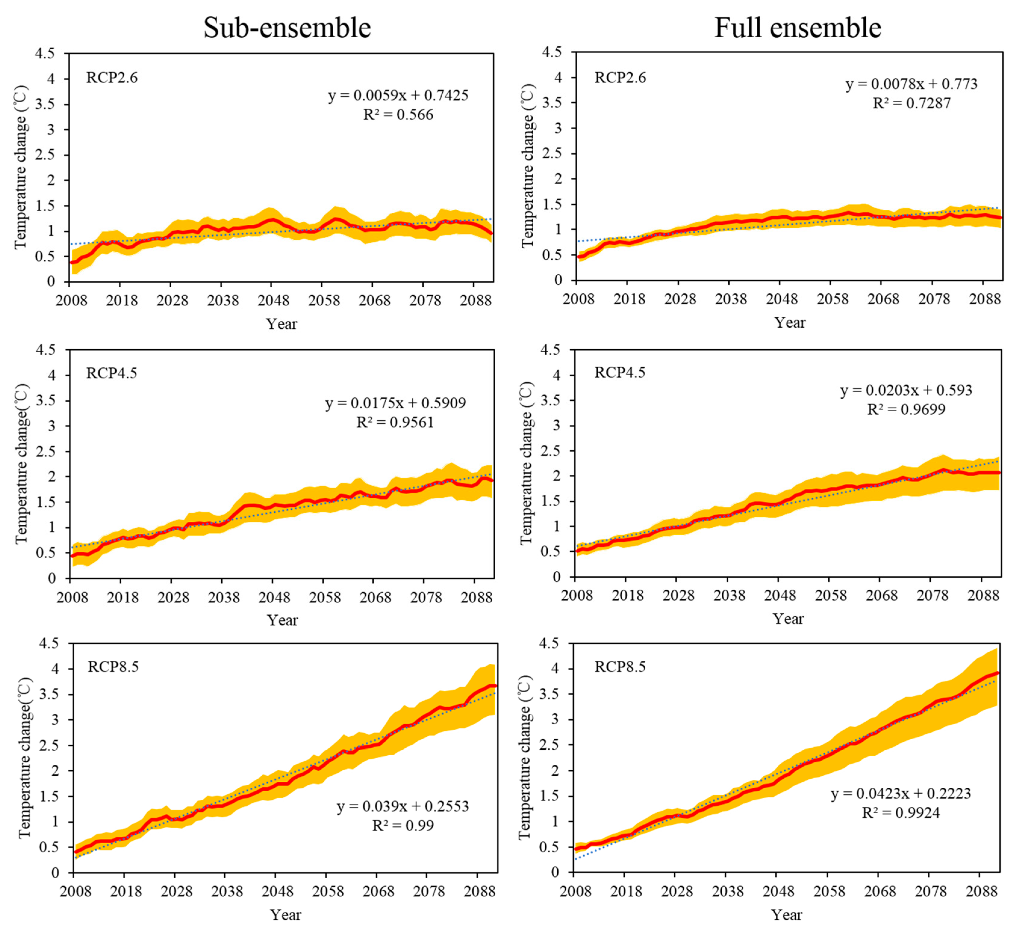
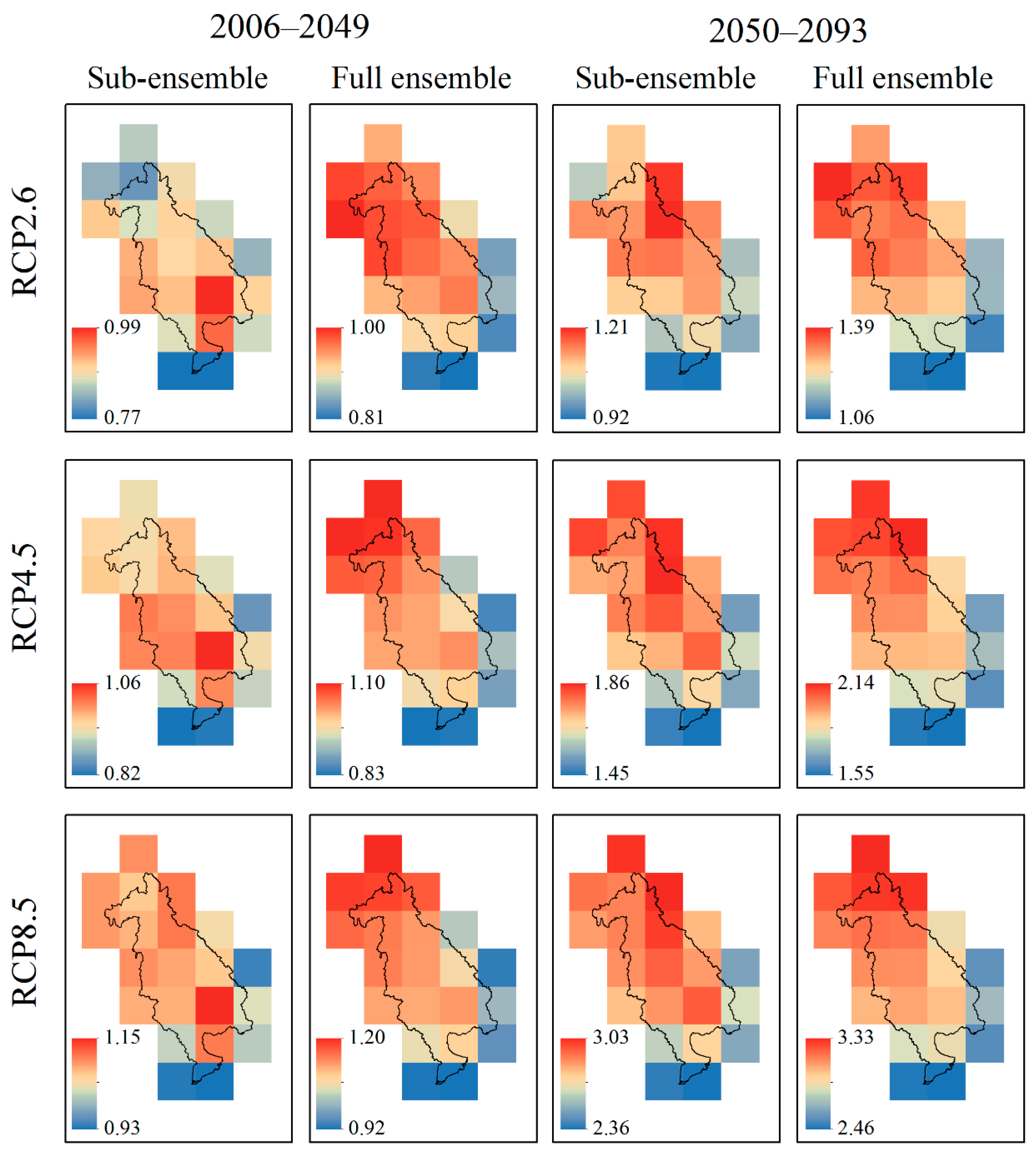
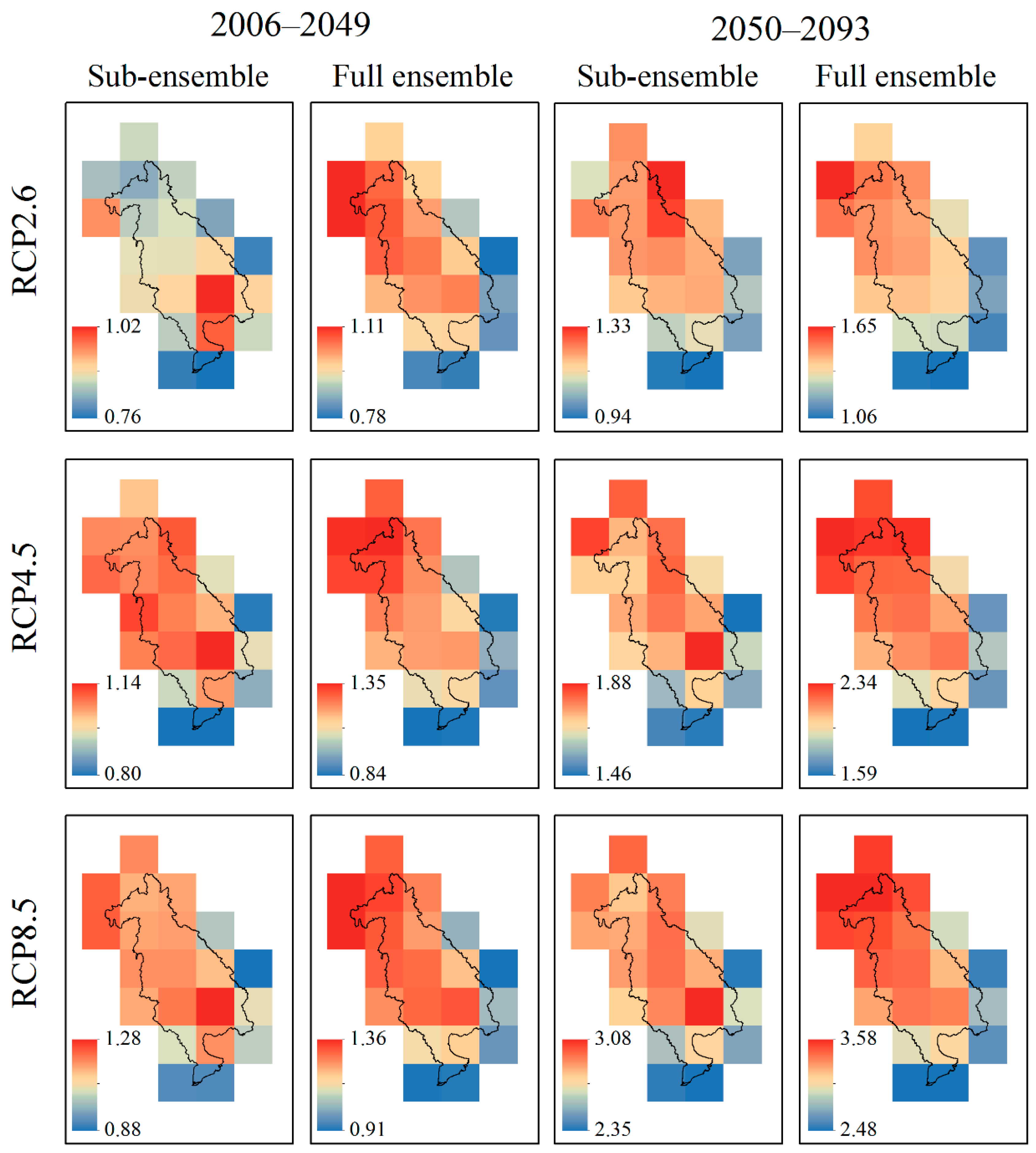
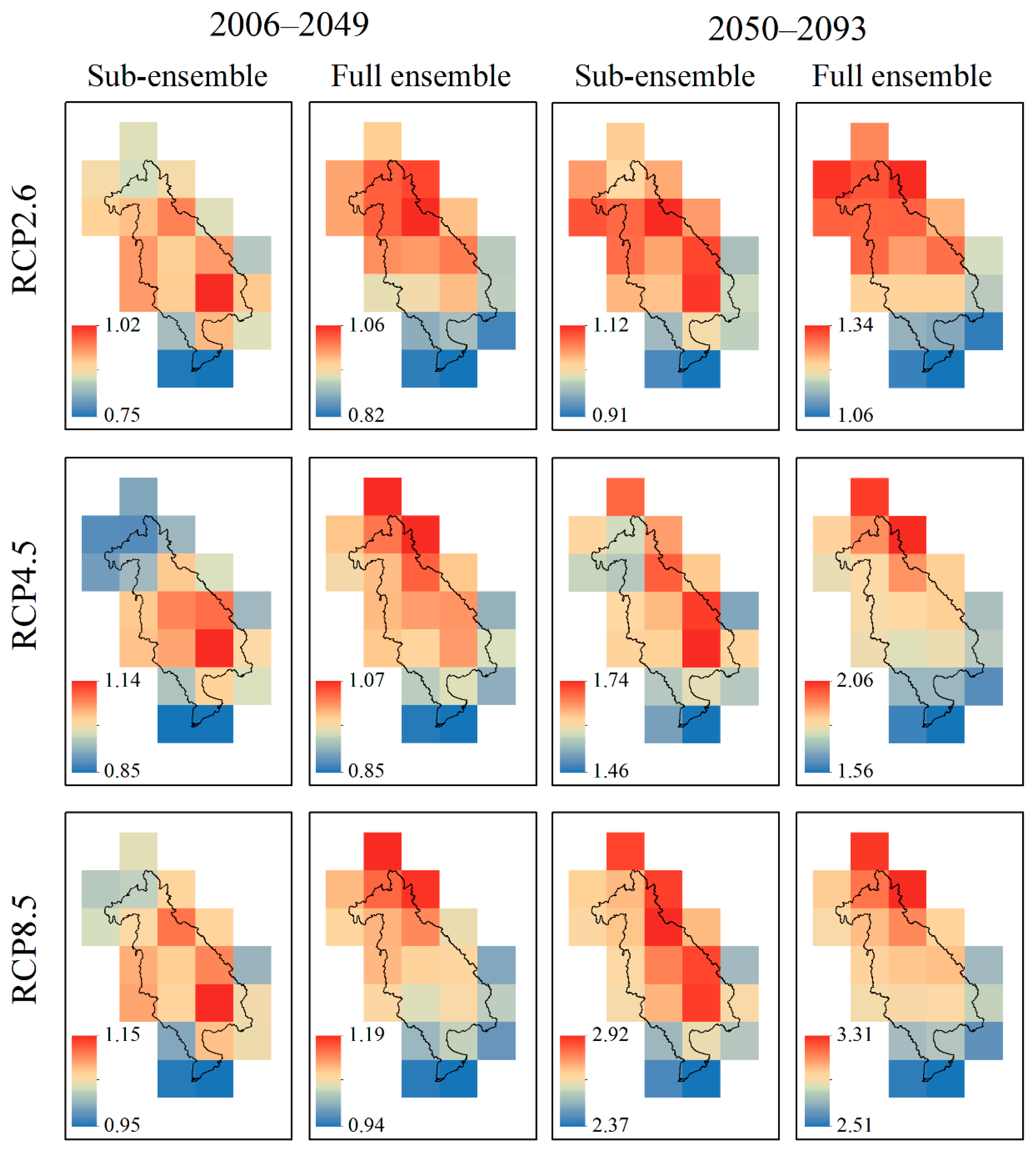
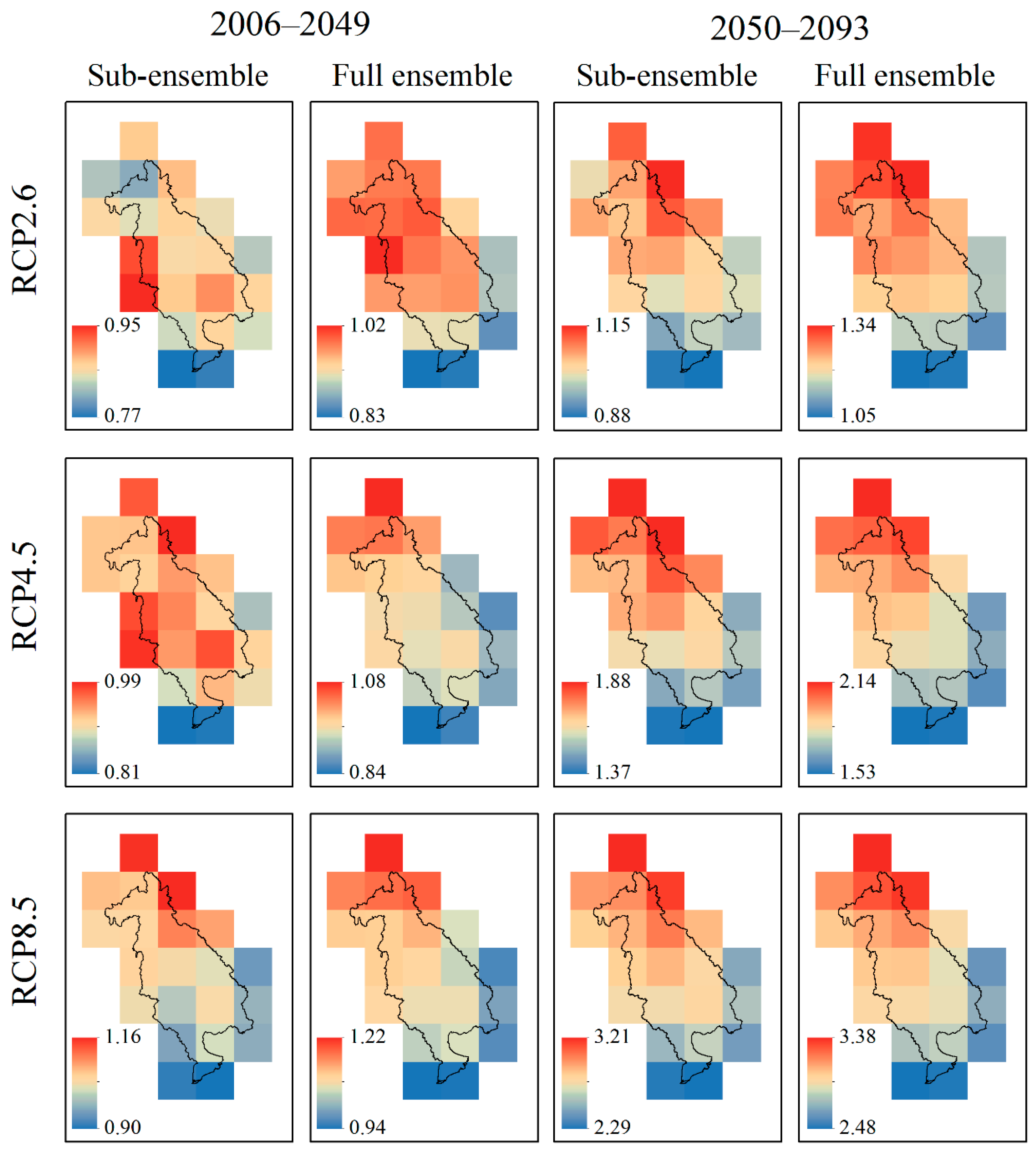
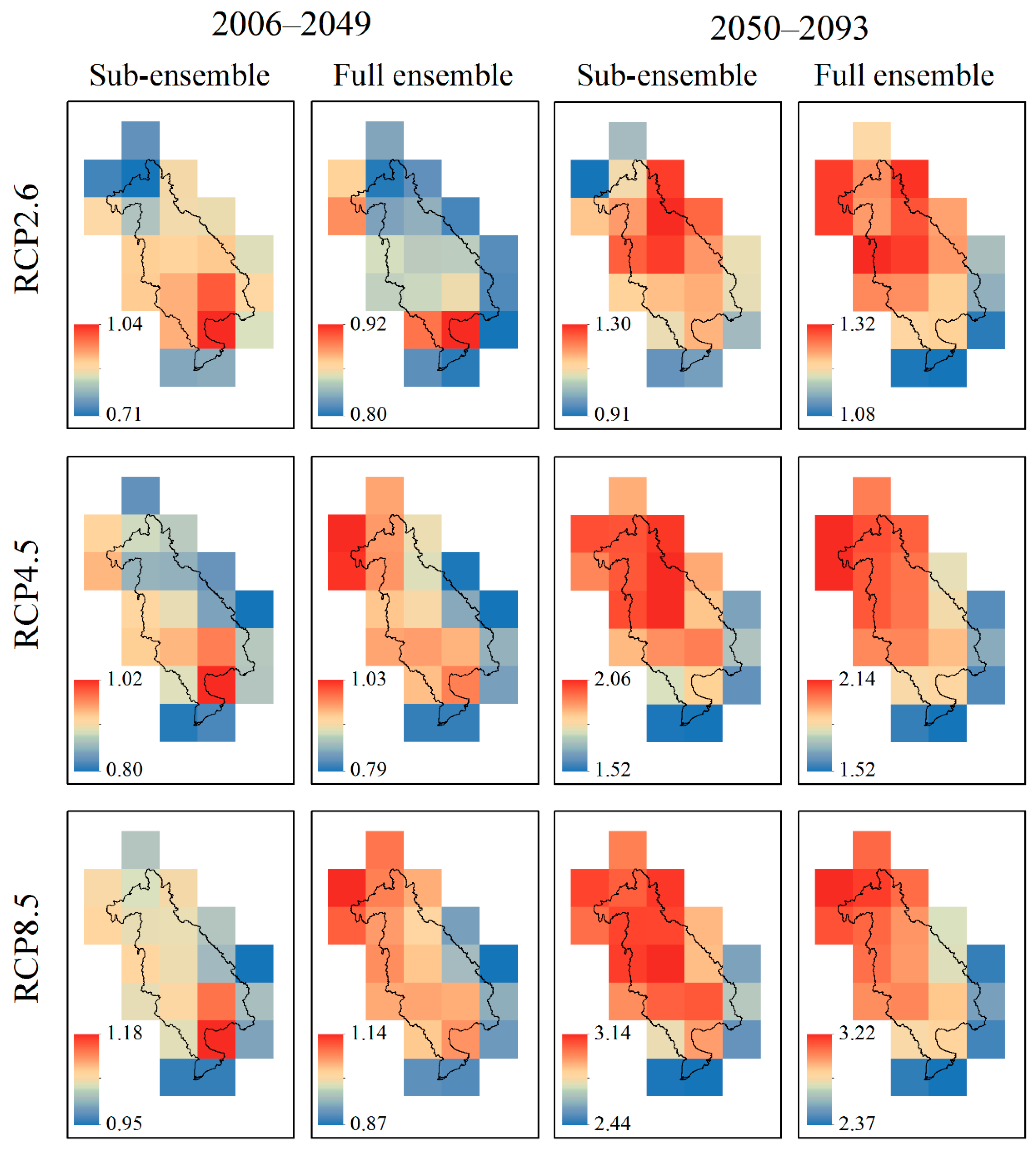
3.5. Future Temperature Projection
4. Discussion
5. Conclusions
Author Contributions
Funding
Conflicts of Interest
References
- IPCC. Climate Change 2013—The Physical Science Basis by Intergovernmental Panel on Climate Change; Cambridge University Press (CUP): Cambridge, UK, 2009. [Google Scholar]
- Eastham, J.; Mpelasoka, F.; Mainuddin, M.; Ticehurst, C.; Dyce, P.; Hodgson, G.; Ali, R.; Kirby, M. Mekong River Basin Water Resources Assessment: Impacts of Climate Change; Water for a Healthy Country National Research Flagship Report; CSIRO: Canberra, Australia, 2008. [Google Scholar]
- Qin, D.H.; Luo, Y.; Chen, Z.L.; Ren, J.W.; Shen, Y.P. Latest advances in climate change sciences: Interpretation of the synthesis report of the IPCC fourth assessment report. Adv. Climate. Change. Res. 2007, 3, 311–314. (In Chinese) [Google Scholar]
- Rupp, D.E.; Abatzoglou, J.T.; Hegewisch, K.C.; Mote, P.W. Evaluation of CMIP5 20th century climate simulations for the Pacific Northwest USA. J. Geophys. Res. Atmos. 2013, 118, 10884–10906. [Google Scholar] [CrossRef]
- Miao, C.Y.; Duan, Q.Y.; Sun, Q.H.; Huang, Y.; Kong, D.X.; Yang, T.T.; Ye, A.Z.; Di, Z.H.; Gong, W. Assessment of CMIP5 climate models and projected temperature changes over Northern Eurasia. Environ. Res. Lett. 2014, 9, 055007. [Google Scholar] [CrossRef]
- Ahmadalipour, A.; Rana, A.; Moradkhani, H.; Sharma, A. Multi-criteria evaluation of CMIP5 GCMs for climate change impact analysis. Theor. Appl. Climatol. 2015, 128, 71–87. [Google Scholar] [CrossRef]
- Dong, T.Y.; Dong, W.J.; Guo, Y.; Chou, J.M.; Yang, S.L.; Tian, D.; Yan, D.D. Future temperature changes over the critical Belt and Road region based on CMIP5 models. Adv. Climate Change Res. 2018, 9, 57–65. [Google Scholar] [CrossRef]
- Das, L.; Dutta, M.; Mezghani, A.; Benestad, R.E. Use of observed temperature statistics in ranking CMIP5 model performance over the Western Himalayan Region of India. Int. J. Climatol. 2017, 38, 554–570. [Google Scholar] [CrossRef]
- Sun, Q.H.; Miao, C.Y.; Duan, Q.Y. Comparative analysis of CMIP3 and CMIP5 global climate models for simulating the daily mean, maximum, and minimum temperatures and daily precipitation over China. J. Geophys. Res. Atmos. 2015, 120, 4806–4824. [Google Scholar] [CrossRef]
- Koutroulis, A.G.; Grillakis, M.G.; Tsanis, I.K.; Papadimitriou, L. Evaluation of precipitation and temperature simulation performance of the CMIP3 and CMIP5 historical experiments. Clim. Dyn. 2015, 47, 1881–1898. [Google Scholar] [CrossRef]
- Guo, Y.; Dong, W.J.; Ren, F.M.; Zhao, Z.C.; Huang, J.B. Surface Air Temperature Simulations over China with CMIP5 and CMIP3. Adv. Climate Change Res. 2013, 4, 145–152. [Google Scholar]
- Sonali, P.; Kumar, D.N.; Nanjundiah, R.S. Intercomparison of CMIP5 and CMIP3 simulations of the 20th century maximum and minimum temperatures over India and detection of climatic trends. Meteorol. Atmos. Phys. 2016, 128, 465–489. [Google Scholar] [CrossRef]
- Lee, Y.-Y.; Black, R.X. Boreal winter low-frequency variability in CMIP5 models. J. Geophys. Res. Atmos. 2013, 118, 6891–6904. [Google Scholar] [CrossRef]
- Ning, L.; Bradley, R.S. NAO and PNA influences on winter temperature and precipitation over the eastern United States in CMIP5 GCMs. Clim. Dyn. 2015, 46, 1257–1276. [Google Scholar] [CrossRef]
- Wang, X.; Chen, M.; Wang, C.; Yeh, S.-W.; Tan, W. Evaluation of performance of CMIP5 models in simulating the North Pacific Oscillation and El Niño Modoki. Clim. Dyn. 2018, 1–12. [Google Scholar] [CrossRef]
- Hawkins, E.; Sutton, R. The Potential to Narrow Uncertainty in Regional Climate Predictions. Bull. Amer. Meteor. Soc. 2009, 90, 1095–1108. [Google Scholar] [CrossRef]
- Bannister, D.; Herzog, M.; Graf, H.-F.; Hosking, J.S.; Short, C.A. An Assessment of Recent and Future Temperature Change over the Sichuan Basin, China, Using CMIP5 Climate Models. J. Clim. 2017, 30, 6701–6722. [Google Scholar] [CrossRef]
- Abbasian, M.; Moghim, S.; Abrishamchi, A. Performance of the general circulation models in simulating temperature and precipitation over Iran. Meteorol. Atmos. Phys. 2018, 1–19. [Google Scholar] [CrossRef]
- Robock, A.; Turco, R.P.; Harwell, M.A.; Ackerman, T.P.; Andressen, R.; Chang, H.-S.; Sivakumar, M.V.K. Use of general circulation model output in the creation of climate change scenarios for impact analysis. Climatic Change 1993, 23, 293–335. [Google Scholar] [CrossRef]
- Risbey, J.S.; Stone, P.H. A Case Study of the Adequacy of GCM Simulations for Input to Regional Climate Change Assessments. J. Clim. 1996, 9, 1441–1467. [Google Scholar] [CrossRef]
- Xu, Y.; Xu, C.; Gao, X.; Luo, Y. Projected changes in temperature and precipitation extremes over the Yangtze River Basin of China in the 21st century. Quat. Int. 2009, 208, 44–52. [Google Scholar] [CrossRef]
- Luo, M.; Liu, T.; Frankl, A.; Duan, Y.; Meng, F.; Bao, A.; Kurban, A.; De Maeyer, P. Defining spatiotemporal characteristics of climate change trends from downscaled GCMs ensembles: How climate change reacts in Xinjiang, China. Int. J. Climatol. 2018, 38, 2538–2553. [Google Scholar] [CrossRef]
- Fan, L.J.; Fu, C.B.; Chen, D.L. Review on creating future climate change scenarios by statistical downscaling techniques. Adv. Earth. Sci. 2008, 20, 320–329. (In Chinese) [Google Scholar]
- Choi, W.; Rasmussen, P.F.; Moore, A.R.; Kim, S.J. Simulating streamflow response to climate scenarios in central Canada using a simple statistical downscaling method. Clim. Res. 2009, 40, 89–102. [Google Scholar] [CrossRef]
- Liu, L.; Liu, Z.; Ren, X.; Fischer, T.; Xu, Y. Hydrological impacts of climate change in the Yellow River Basin for the 21st century using hydrological model and statistical downscaling model. Quat. Int. 2011, 244, 211–220. [Google Scholar] [CrossRef]
- Horton, R.M.; Gornitz, V.; Bader, D.A.; Goldberg, R.; Ruane, A.C.; Rosenzweig, C. Climate Hazard Assessment for Stakeholder Adaptation Planning in New York City. J. Appl. Meteor. Climatol. 2011, 50, 2247–2266. [Google Scholar] [CrossRef]
- Rahimi, J.; Ebrahimpour, M.; Khalili, A. Spatial changes of Extended De Martonne climatic zones affected by climate change in Iran. Theor. Appl. Climatol. 2012, 112, 409–418. [Google Scholar] [CrossRef]
- Wang, T.; Hamann, A.; Spittlehouse, D.; Carroll, C. Locally Downscaled and Spatially Customizable Climate Data for Historical and Future Periods for North America. PLoS ONE 2016, 11, 0156720. [Google Scholar] [CrossRef] [PubMed]
- Walsh, J.E.; Bhatt, U.S.; Littell, J.S.; Leonawicz, M.; Lindgren, M.; Kurkowski, T.A.; Bieniek, P.A.; Thoman, R.; Gray, S.; Rupp, T.S. Downscaling of climate model output for Alaskan stakeholders. Environ. Model. Software 2018, 110, 38–51. [Google Scholar] [CrossRef]
- Trisurat, Y.; Aekakkararungroj, A.; Ma, H.-O.; Johnston, J.M. Basin-wide impacts of climate change on ecosystem services in the Lower Mekong Basin. Ecol. Res. 2017, 33, 73–86. [Google Scholar] [CrossRef] [PubMed]
- Mekong River Commission; ICEM. MRC: Vulnerability Report Volume 2: Basin-Wide Climate Change Impact and Vulnerability Assessment for Wetland Dependent Livelihoods and Eco-Services; Mekong River Commission: Vientiane, Laos; ICEM: Melbourne, Australia, 2015. [Google Scholar]
- Hoanh, C.T.; Jirayoot, K.; Lacombe, G.; Srinetr, V. Impacts of Climate Change and Development on Mekong Flow Regimes. First Assessment—2009; International Water Management Institute: Colombo, Sri Lanka, 2010. [Google Scholar]
- Yoshimura, C.; Zhou, M.; Kiem, A.S.; Fukami, K.; Prasantha, H.H.; Ishidaira, H.; Takeuchi, K. 2020s scenario analysis of nutrient load in the Mekong River Basin using a distributed hydrological model. Sci. Total Environ. 2009, 407, 5356–5366. [Google Scholar] [CrossRef]
- Kingston, D.G.; Thompson, J.R.; Kite, G. Uncertainty in climate change projections of discharge for the Mekong River Basin. Hydrol. Earth Syst. Sci. 2011, 15, 1459–1471. [Google Scholar] [CrossRef]
- Huang, Y.; Wang, F.; Li, Y.; Cai, T. Multi-model ensemble simulation and projection in the climate change in the Mekong River Basin. Part I: Temperature. Environ. Monit. Assess. 2014, 186, 7513–7523. [Google Scholar] [CrossRef] [PubMed]
- Taylor, K.E.; Stouffer, R.J.; Meehl, G.A. An Overview of CMIP5 and the Experiment Design. Bull. Amer. Meteor. Soc. 2012, 93, 485–498. [Google Scholar] [CrossRef]
- Yasutomi, N.; Hamada, A.; Yatagai, A. Development of a long-term daily gridded temperature dataset and its application to rain/snow discrimination of daily precipitation. Global. Environ. Res. 2011, 15, 165–172. [Google Scholar]
- Lutz, A.; Terink, W.; Droogers, P.; Immerzeel, W.; Piman, T. Development of Baseline Climate Data Set and Trend Analysis in the Mekong Basin; Mekong River Commission: Vientiane, Laos, 2014; pp. 1–127. [Google Scholar]
- Fu, G.; Liu, Z.; Charles, S.P.; Xu, Z.; Yao, Z. A score-based method for assessing the performance of GCMs: A case study of southeastern Australia. J. Geophys. Res. Atmos. 2013, 118, 4154–4167. [Google Scholar] [CrossRef]
- Liu, Z.F.; Wang, R.; Yao, Z.J. Air temperature and precipitation over the Mongolian Plateau and assessment of CMIP5 climate models. Resour. Sci. 2016, 38, 956–969. (In Chinese) [Google Scholar]
- Mann, H.B. Nonparametric tests against trend. Econometrica 1945, 13, 245–259. [Google Scholar] [CrossRef]
- Kendall, M.G. Rank Correlation Methods, 4th ed.; Charles Griffin: London, UK, 1975. [Google Scholar]
- Hirsch, R.M.; Alexander, R.B.; Smith, R.A. Selection of methods for the detection and estimation of trends in water quality. Water Resour. Res. 1991, 27, 803–813. [Google Scholar] [CrossRef]
- Sen, P.K. Estimates of the regression coefficient based on Kendall’s tau. J. Am. Stat. Assoc. 1968, 63, 1379–1389. [Google Scholar] [CrossRef]
- Hirsch, R.M.; Slack, J.R.; Smith, R.A. Techniques of trend analysis for monthly water quality data. Water Resour. Res. 1982, 18, 107–121. [Google Scholar] [CrossRef]
- Perkins, S.E.; Pitman, A.; Holbrook, N.J.; McAneney, J. Evaluation of the AR4 Climate Models’ Simulated Daily Maximum Temperature, Minimum Temperature, and Precipitation over Australia Using Probability Density Functions. J. Clim. 2007, 20, 4356–4376. [Google Scholar] [CrossRef]
- Hu, Q.; Jiang, D.B.; Fan, G.Z. Evaluation of CMIP5 models over the Qinghai-Tibetan Plateau. Chin. J. Atmosph. Sci. 2014, 38, 924–938. (In Chinese) [Google Scholar]
- Zazulie, N.; Rusticucci, M.; Raga, G.B. Regional climate of the subtropical central Andes using high-resolution CMIP5 models—Part I: Past performance (1980–2005). Clim. Dyn. 2017, 49, 3937–3957. [Google Scholar] [CrossRef]
- Kumar, D.; Kodra, E.; Ganguly, A.R. Regional and seasonal intercomparison of CMIP3 and CMIP5 climate model ensembles for temperature and precipitation. Clim. Dyn. 2014, 43, 2491–2518. [Google Scholar] [CrossRef]
- Venkataraman, K.; Tummuri, S.; Medina, A.; Perry, J. 21st century drought outlook for major climate divisions of Texas based on CMIP5 multimodel ensemble: Implications for water resource management. J. Hydrol. 2016, 534, 300–316. [Google Scholar] [CrossRef]
- Ahmadalipour, A.; Moradkhani, H.; Rana, A. Accounting for downscaling and model uncertainty in fine-resolution seasonal climate projections over the Columbia River Basin. Clim. Dyn. 2017, 50, 717–733. [Google Scholar] [CrossRef]
- Wang, X.; Yang, T.; Li, X.; Shi, P.; Zhou, X. Spatio-temporal changes of precipitation and temperature over the Pearl River basin based on CMIP5 multi-model ensemble. Stoch. Environ. Res. Risk Assess. 2016, 31, 1077–1089. [Google Scholar] [CrossRef]


| Model Name | ID | Institution | Resolution (Lon × Lat) |
|---|---|---|---|
| ACCESS1.0 | 1 | Commonwealth Scientific and Industrial Research Organization and Bureau of Meteorology, Australia | 1.88° × 1.25° |
| ACCESS1.3 | 2 | 1.88° × 1.25° | |
| BCC-CSM1.1 | 3 | Beijing Climate Center, China Meteorological Administration, China | 2.81° × 2.79° |
| BNU-ESM | 4 | College of Global Change and Earth System Science, Beijing Normal University, China | 2.81° × 2.79° |
| CanESM2 | 5 | Canadian Centre for Climate Modelling and Analysis, Canada | 2.81° × 2.79° |
| CCSM4 | 6 | National Center for Atmospheric Research, USA | 1.25° × 0.94° |
| CESM1(CAM5) | 7 | 1.25° × 0.94° | |
| CESM1(WACCM) | 8 | 2.50° × 1.88° | |
| CMCC-CMS | 9 | Centro Euro-Mediterraneo sui Cambiamenti Climatici, Italy | 1.88° × 1.88° |
| CNRM-CM5 | 10 | Centre National de Recherches Météorologiques Centre Européen de Recherche et Formation Avancée en Calcul Scientifique, France | 1.41° × 1.40° |
| CSIRO-Mk3.6.0 | 11 | Commonwealth Scientific and Industrial Research Organization/Queensland Climate Change Centre of Excellence | 1.88° × 1.88° |
| EC-EARTH | 12 | EC-EARTH consortium published at Irish Centre for High-End Computing, Netherlands/Ireland | 1.13° × 1.13° |
| FGOALS-g2 | 13 | Atmospheric Sciences and Geophysical Fluid Dynamics/Institute of Atmospheric Physics, Chinese Academy of Sciences, China | 2.81° × 2.81° |
| FIO-ESM | 14 | The First Institute of Oceanography, SOA, China | 2.80° × 2.80° |
| GFDL-CM3 | 15 | NOAA Geophysical Fluid Dynamics Laboratory, USA | 2.50° × 2.00° |
| GFDL-ESM2G | 16 | 2.00° × 2.02° | |
| GFDL-ESM2M | 17 | 2.50° × 2.02° | |
| GISS-E2-H | 18 | NASA/GISS (Goddard Institute for Space Studies), USA | 2.50° × 2.00° |
| GISS-E2-R | 19 | 2.50° × 2.00° | |
| HadGEM2-AO | 20 | National Institute of Meteorological Research, Korea Meteorological Administration, Korea | 1.88° × 1.25° |
| HadGEM2-CC | 21 | Met Office Hadley Center, UK | 1.88° × 1.25° |
| HadGEM2-ES | 22 | 1.88° × 1.25° | |
| INMCM4.0 | 23 | Russian Academy of Sciences, Institute for Numerical Mathematics, Russia | 2.00° × 1.50° |
| IPSL-CM5A-LR | 24 | Institute Pierre-Simon Laplace, France | 3.75° × 1.89° |
| IPSL-CM5A-MR | 25 | 2.50° × 1.27° | |
| IPSL-CM5B-LR | 26 | 3.75° × 1.89° | |
| MIROC4h | 27 | Atmosphere and Ocean Research Institute (The University of Tokyo), National Institute for Environmental Studies, and Japan Agency | 0.56° × 0.56° |
| MIROC5 | 28 | for Marine-Earth Science and Technology, Japan | 1.41° × 1.40° |
| MIROC-ESM | 29 | 2.81° × 2.79° | |
| MIROC-ESM-CHEM | 30 | 2.81° × 2.79° | |
| MPI-ESM-LR | 31 | Max Planck Institute for Meteorology, Germany | 1.88° × 1.87° |
| MPI-ESM-MR | 32 | 1.88° × 1.87° | |
| MRI-CGCM3 | 33 | Meteorological Research Institute, Japan | 1.13° × 1.12° |
| NorESM1-M | 34 | Bjerknes Centre for Climate Research, Norwegian Climate Center, Norway | 2.50° × 1.89° |
| ID | Means (°C) | SD | NRMSE | r | Trend | Sscore | |
|---|---|---|---|---|---|---|---|
| Z | Sen’s slope (°C/yr) | ||||||
| Obs | 24.62 | 2.13 | 2.80 | 0.01 | |||
| 1 | 25.49 | 2.94 | 0.81 | 0.952 | 3.15 | 0.013 | 0.62 |
| 2 | 25.44 | 3.77 | 1.04 | 0.972 | 1.18 | 0.0072 | 0.55 |
| 3 | 23.63 | 2.88 | 0.77 | 0.896 | 3.04 | 0.0123 | 0.61 |
| 4 | 23.68 | 3.21 | 0.84 | 0.886 | 2.42 | 0.0125 | 0.65 |
| 5 | 24.48 | 2.14 | 0.52 | 0.874 | 4.00 | 0.0215 | 0.53 |
| 6 | 22.73 | 3.18 | 1.12 | 0.897 | 2.54 | 0.0138 | 0.66 |
| 7 | 22.57 | 2.71 | 1.12 | 0.904 | 1.57 | 0.0096 | 0.65 |
| 8 | 23.51 | 2.58 | 0.74 | 0.876 | 2.17 | 0.0101 | 0.62 |
| 9 | 25.00 | 3.06 | 0.84 | 0.930 | 3.04 | 0.0233 | 0.60 |
| 10 | 23.08 | 2.73 | 0.93 | 0.910 | 3.35 | 0.0132 | 0.66 |
| 11 | 23.82 | 3.54 | 0.92 | 0.929 | 2.30 | 0.0098 | 0.59 |
| 12 | 22.13 | 1.57 | 1.30 | 0.930 | 3.35 | 0.0149 | 0.62 |
| 13 | 22.86 | 2.52 | 1.03 | 0.883 | 4.00 | 0.0223 | 0.65 |
| 14 | 23.65 | 3.36 | 0.88 | 0.901 | 2.78 | 0.0157 | 0.60 |
| 15 | 22.94 | 2.91 | 1.03 | 0.972 | 1.81 | 0.0088 | 0.51 |
| 16 | 22.41 | 3.30 | 1.32 | 0.947 | 3.55 | 0.0213 | 0.53 |
| 17 | 22.88 | 3.34 | 1.18 | 0.959 | 2.78 | 0.0213 | 0.51 |
| 18 | 23.90 | 2.57 | 0.63 | 0.927 | 2.58 | 0.0096 | 0.70 |
| 19 | 24.35 | 2.46 | 0.54 | 0.922 | 2.50 | 0.0111 | 0.64 |
| 20 | 25.68 | 3.09 | 0.88 | 0.939 | 2.76 | 0.0143 | 0.61 |
| 21 | 24.42 | 3.04 | 0.74 | 0.919 | 3.57 | 0.0155 | 0.60 |
| 22 | 24.79 | 3.04 | 0.74 | 0.933 | 2.68 | 0.011 | 0.59 |
| 23 | 21.60 | 3.13 | 1.57 | 0.829 | 2.68 | 0.0133 | 0.51 |
| 24 | 22.89 | 2.94 | 1.01 | 0.915 | 4.30 | 0.0186 | 0.64 |
| 25 | 23.49 | 3.08 | 0.84 | 0.916 | 5.23 | 0.0219 | 0.62 |
| 26 | 22.92 | 2.86 | 0.97 | 0.903 | 4.72 | 0.021 | 0.66 |
| 27 | 24.42 | 3.03 | 0.62 | 0.936 | 5.27 | 0.0228 | 0.67 |
| 28 | 24.25 | 2.82 | 0.60 | 0.947 | 0.31 | 0.0026 | 0.69 |
| 29 | 23.82 | 3.15 | 0.79 | 0.933 | 3.73 | 0.0189 | 0.57 |
| 30 | 23.87 | 3.14 | 0.79 | 0.931 | 2.52 | 0.0141 | 0.57 |
| 31 | 24.18 | 3.13 | 0.75 | 0.932 | 3.49 | 0.0226 | 0.61 |
| 32 | 24.28 | 3.17 | 0.75 | 0.925 | 2.48 | 0.0156 | 0.63 |
| 33 | 22.88 | 3.21 | 1.09 | 0.934 | 3.53 | 0.014 | 0.59 |
| 34 | 22.00 | 3.14 | 1.41 | 0.884 | 2.84 | 0.0135 | 0.62 |
| Period | RCP2.6 | RCP4.5 | RCP8.5 | ||||||||||||
|---|---|---|---|---|---|---|---|---|---|---|---|---|---|---|---|
| Annual | MAM | JJA | SON | DJF | Annual | MAM | JJA | SON | DJF | Annual | MAM | JJA | SON | DJF | |
| 2006–2049 | 0.87 (0.93) | 0.86 (0.97) | 0.89 (0.95) | 0.85 (0.95) | 0.87 (0.84) | 0.95 (0.99) | 1.01 (1.14) | 0.97 (0.98) | 0.92 (0.95) | 0.88 (0.91) | 1.06 (1.09) | 1.12 (1.18) | 1.05 (1.07) | 1.02 (1.07) | 1.04 (1.02) |
| 2050–2093 | 1.09 (1.26) | 1.16 (1.37) | 1.04 (1.22) | 1.03 (1.22) | 1.13 (1.23) | 1.70 (1.90) | 1.70 (2.07) | 1.61 (1.80) | 1.65 (1.84) | 1.86 (1.90) | 2.78 (2.97) | 2.76 (3.17) | 2.69 (2.92) | 2.76 (2.93) | 2.91 (2.86) |
© 2019 by the authors. Licensee MDPI, Basel, Switzerland. This article is an open access article distributed under the terms and conditions of the Creative Commons Attribution (CC BY) license (http://creativecommons.org/licenses/by/4.0/).
Share and Cite
Ruan, Y.; Liu, Z.; Wang, R.; Yao, Z. Assessing the Performance of CMIP5 GCMs for Projection of Future Temperature Change over the Lower Mekong Basin. Atmosphere 2019, 10, 93. https://doi.org/10.3390/atmos10020093
Ruan Y, Liu Z, Wang R, Yao Z. Assessing the Performance of CMIP5 GCMs for Projection of Future Temperature Change over the Lower Mekong Basin. Atmosphere. 2019; 10(2):93. https://doi.org/10.3390/atmos10020093
Chicago/Turabian StyleRuan, Yunfeng, Zhaofei Liu, Rui Wang, and Zhijun Yao. 2019. "Assessing the Performance of CMIP5 GCMs for Projection of Future Temperature Change over the Lower Mekong Basin" Atmosphere 10, no. 2: 93. https://doi.org/10.3390/atmos10020093
APA StyleRuan, Y., Liu, Z., Wang, R., & Yao, Z. (2019). Assessing the Performance of CMIP5 GCMs for Projection of Future Temperature Change over the Lower Mekong Basin. Atmosphere, 10(2), 93. https://doi.org/10.3390/atmos10020093