Estimating Maximum Daily Precipitation in the Upper Vistula Basin, Poland

Abstract

The aim of this study was to determine the best probability distributions for calculating the maximum annual daily precipitation with the specific probability of exceedance (P_maxp%). The novelty of this study lies in using the peak-weighted root mean square error (PWRMSE), the root mean square error (RMSE), and the coefficient of determination (R²) for assessing the fit of empirical and theoretical distributions. The input data included maximum daily precipitation records collected in the years 1971–2014 at 51 rainfall stations from the Upper Vistula Basin, Southern Poland. The value of P_maxp% was determined based on the following probability distributions of random variables: Pearson’s type III (PIII), Weibull’s (W), log-normal, generalized extreme value (GEV), and Gumbel’s (G). Our outcomes showed a lack of significant trends in the observation series of the investigated random variables for a majority of the rainfall stations in the Upper Vistula Basin. We found that the peak-weighted root mean square error (PWRMSE) method, a commonly used metric for quality assessment of rainfall-runoff models, is useful for identifying the statistical distributions of the best fit. In fact, our findings demonstrated the consistency of this approach with the RMSE goodness-of-fit metrics. We also identified the GEV distribution as recommended for calculating the maximum daily precipitation with the specific probability of exceedance in the catchments of the Upper Vistula Basin.

1. Introduction

The analysis of the maximum annual daily precipitation (P_max) is one of the crucial factors for the management of water resources in a catchment [1]. By knowing the probability and frequency of such precipitation, decision-makers are able to mitigate the effects of floods. In fact, determining the maximum annual daily precipitation with a specific probability of exceedance (P_maxp%) is necessary to tackle the issues of excessive or deficient precipitation and, thus, to meet regional water needs. The estimation of P_maxp% is also important for determining flood hazard zones, for designing specific hydraulic structures or systems [2] or for assessing the performance of sewage treatment plants under variable weather conditions [3]. However, the growing atmospheric content of greenhouse gases and the resulting global warming we have been experiencing for a few decades significantly affected the precipitation structure (height and spatial variability), thus making the prediction of P_maxp% increasingly difficult [4,5,6].

Based on a sufficiently long observation series of the maximum annual daily precipitation, it is possible to predict P_maxp% by using probability distributions of random variables. In hydrological studies, P_maxp% is commonly determined by using the following probability distribution functions: normal distribution, log-normal distribution, Pearson’s type III, exponential function, Gumbel’s distribution, generalized extreme value distribution (GEV), and Weibull’s and Pareto’s distributions [7,8,9,10,11,12,13]. Wdowikowski et al. [14] recommend the generalized exponential distribution for such a purpose. In [15,16], it is shown that hydrological records of typical length (some decades) may display a distorted picture of the actual distribution, suggesting that the Gumbel distribution is not an appropriate model for rainfall extremes. In addition, it is therein demonstrated that the extreme value distribution of type II (EV2) is a more consistent alternative. Selecting an appropriate form of probability distribution involves matching a proper theoretical function with an empirical distribution of a random variable. The selection of an inappropriate function for a region may result in underestimating or overestimating the maximum hydro-meteorological events with a specific probability of exceedance [17].

The application of model selection criteria within the field of frequency analysis of hydrological extremes is rare [18]. The only methods are Akaike (AIC) or Schwartz (BIC) information criteria [19]. Also, alternative statistical tests could be employed for assessing the performance of theoretical distributions, such as, for instance, the Anderson–Darling, which compares the whole range but gives more weight to the upper tail [20]. The main disadvantage of these goodness-of-fit metrics is that they do not provide information on the accuracy limit and on the inclusion of atypical (outlying) values. Moreover, it is not possible to assess the value of the test statistics. On the other hand, methods commonly used for assessing the quality of rainfall-runoff hydrological models, such as the percentage error in peak flow, percentage error in volume, efficiency coefficient, peak-weighted root mean square error, the sum of absolute residuals, or the sum of squared residuals, seem promising alternatives. In fact, some of them, e.g., the efficiency coefficient, can be assessed against a scale indicating the quality of the results yielded by the models [21,22,23,24]. Another option is a known but infrequently used goodness-of-fit metric based on the probability plot correlation coefficient [25,26]. This approach allows for determining the strength of the relationship between the observed and calculated variables using statistical distributions, e.g., the Guilford’s scale [27]. It also shows the statistical significance of the resulting correlation coefficients, thus providing more information on the quality of fit of the probability distributions.

Previous studies focusing on the form of the probability distribution for P_maxp% estimation only tend to achieve the best fit of the theoretical and empirical distributions and to describe the spatial variability of the forms of the probability distributions [28,29,30]. The application of alternative methods (e.g., those used for rainfall-runoff modeling) for assessing the quality of fit of statistical and empirical distribution is not documented in the literature. Hence, the aim of this study was to determine the best probability distributions used for assessing P_maxp%. The novelty of this work consists of identifying the best-fitting theoretical function by adopting the peak-weighted root mean square error (PWRMSE), commonly used for calibrating parameters in hydrological models. Additionally, the root mean square error (RMSE) and the coefficient of determination (R²) were used as the goodness-of-fit metrics. Finally, the study aimed at determining the trend significance for the P_max observation series and at estimating the density function for the stations showing a significant trend.

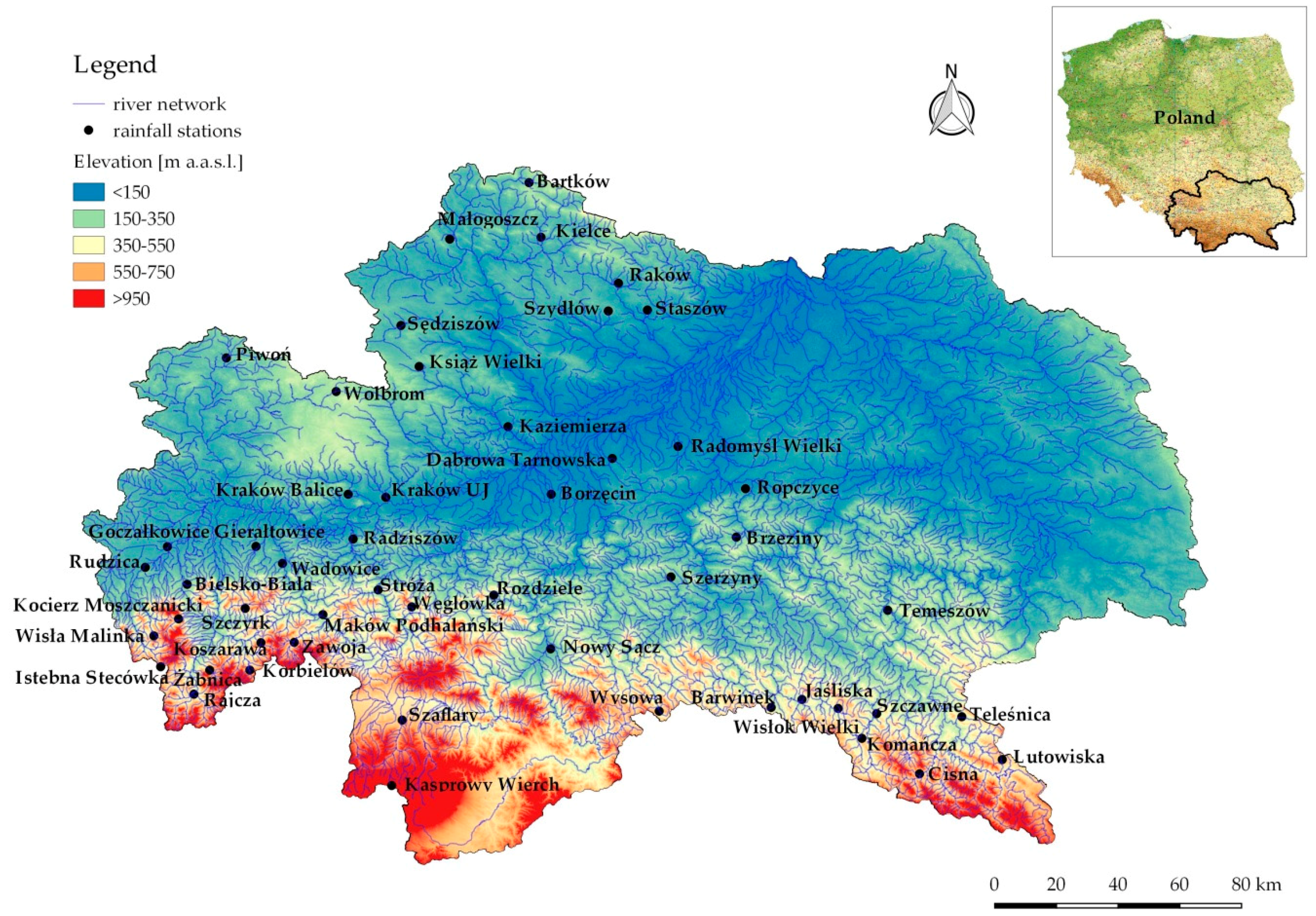
2. Description of the Study Area

The study area is the Upper Vistula Basin, which accounts for about 25% of the entire Vistula basin and about 15% of Poland’s area, and occupies the southern part of the country. It covers part of the Carpathians, the Subcarpathian Valleys and Małopolska Uplands. The study area shows large variations in altitude, and this influences the height of precipitation and its extreme values [31]. The input data were the maximum total daily precipitation recorded in the years 1971–2014 at 51 rainfall stations in the Upper Vistula Basin. The data were obtained from the public database of the Institute of Meteorology and Water Management, National Research Institute in Warsaw. The Upper Vistula Basin and rainfall stations are depicted in Figure 1.

3. Methods

The study involved the following elements: (i) preliminary analysis of the annual maximum precipitation time series, (ii) analysis of trends in the observed series, (iii) determination of the maximum annual daily precipitation with a specific probability of exceedance, (iv) selection of the best fit between theoretical and empirical distribution of random variables.

3.1. Preliminary Analysis of the Observation Series

The preliminary analysis of the annual maximum precipitation included the calculation of descriptive statistics. Specifically, we computed minimum (LP_max), mean (MP_max), and maximum (HP_max) values; measures of dispersion—standard deviation (s) and coefficient of variation (C_s); and measure of shape of the studied variate distribution—the coefficient of skewness (A).

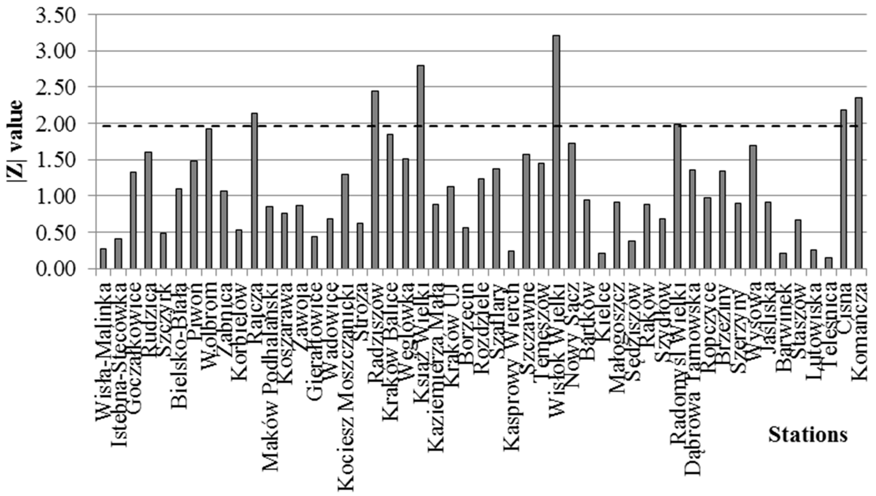
3.2. Analysis of Trends in the Observed Series

Analysis of trends in the observed series was conducted by a Mann-Kendall test. This test was selected due to its advantages with respect to alternative tests. First, in order to apply the Mann-Kendall test, the data need not conform to any particular distribution. Second, the test exhibits low sensitivity to abrupt breaks due to an inhomogeneous time series [32]. The significance level was set to α = 0.05. The H₀ hypothesis of the Mann-Kendall test assumes a lack of a monotonic trend for the data, while the alternative H₁ claims its existence. The S statistics of the Mann-Kendall was based on the following formula [33,34,35,36,37,38]:

$$\mathrm{S}={\sum }_{\mathrm{k}=1}^{\mathrm{n}-1}{\sum }_{\mathrm{j}=\mathrm{k}+1}^{\mathrm{n}}\mathrm{sgn}({\mathrm{x}}_{\mathrm{j}}-{\mathrm{x}}_{\mathrm{k}})$$

(1)

$$\mathrm{sgn}\left({\mathrm{x}}_{\mathrm{j}}-{\mathrm{x}}_{\mathrm{k}}\right)=\{\begin{array}{c}1\mathrm{for}\left({\mathrm{x}}_{\mathrm{j}}-{\mathrm{x}}_{\mathrm{k}}\right)>0\\ 0\mathrm{for}\left({\mathrm{x}}_{\mathrm{j}}-{\mathrm{x}}_{\mathrm{k}}\right)=0\\ -1\mathrm{for}\left({\mathrm{x}}_{\mathrm{j}}-{\mathrm{x}}_{\mathrm{k}}\right)<0\end{array}$$

(2)

where:

• n—the number of elements of the time series,
• x_j—observation at time j,
• x_k—observation at time k.

On the basis of the standard statistics Z calculated according to the formula:

$$\mathrm{Z}=\frac{\mathrm{S}\text{–}\mathrm{sgn}(\mathrm{S})}{{\mathrm{Var}(\mathrm{S})}^{1/2}}$$

(3)

Var(S)—variance S, determined on the basis of the formula:

$$\mathrm{Var}(\mathrm{S})=\frac{1}{18}·(\mathrm{n}·(\mathrm{n}-1)·\left(2·\mathrm{n}+5\right))$$

(4)

where:

• n—the number of elements of the time series.

If the value of Z is lower than the critical value of Z_crit for the assumed significance level α, the hypothesis claiming the lack of a trend is acceptable. Otherwise, the H₀ hypothesis should be discarded in favor of the alternative hypothesis. The main assumption of the used Mann-Kendall test is the lack of autocorrelation in the data series. In the case of the analysis of the maximum annual daily precipitation, such dependencies may occur, which leads to an underestimation of the variance Var (S). Therefore, an adjustment for variance correction is included that is calculated only for data with significant autocorrelation in general [39]:

$$\mathrm{Var}*(\mathrm{S})=\mathrm{Var}(\mathrm{S})·\frac{\mathrm{n}}{{\mathrm{n}}_{\mathrm{s}}^{*}}$$

(5)

where:

• ${\mathrm{n}}_{\mathrm{s}}^{*}$—the effective number of observations calculated as:

$$\frac{\mathrm{n}}{{\mathrm{n}}_{\mathrm{s}}^{*}}=1+\frac{2}{\mathrm{n}(\mathrm{n}-1)(\mathrm{n}-2)}·{\displaystyle \sum _{\mathrm{k}=1}^{\mathrm{n}-1}}(\mathrm{n}-\mathrm{k})(\mathrm{n}-\mathrm{k}-1)(\mathrm{n}-\mathrm{k}-2){\mathsf{\rho }}_{\mathrm{k}}$$

(6)

where:

• ρ_k—the lag k autocorrelation coefficients of the ranks of the observations.

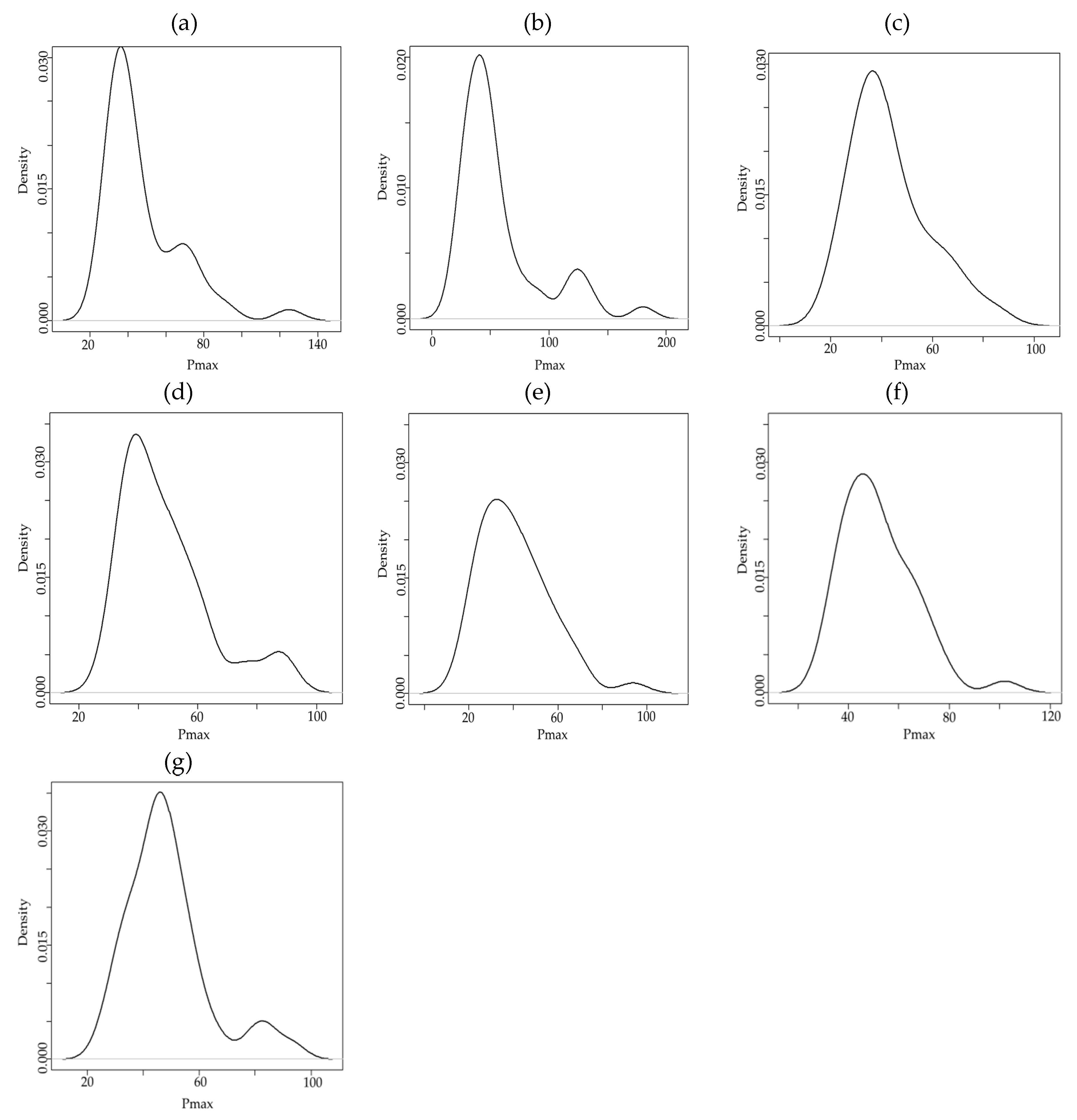
3.3. Identification of Empirical Distributions with Kernel Estimators

For the rainfall stations showing a significant trend, a direct estimation of the unknown density function was made using the kernel estimators. The kernel estimation of the density function is a commonly used tool for analyzing the behavior of hydrological phenomena, including atmospheric precipitation, as evidenced by the works of numerous research teams [40,41,42]. The outcomes allowed us to estimate the variability of the maximum annual daily precipitation. The estimators (${\widehat{f}}_h(\mathrm{x})$) were determined based on the value of an n-element random sample according to the following formula [43,44]:

$${\widehat{f}}_h(x)=\frac{1}{\mathit{nh}}{\sum }_{\mathrm{i}=1}^{n}K(\frac{x-X_i}{n})$$

(7)

where:

• n—sample size;
• h—smoothing parameter equated with so-called band width;
• K—kernel function;
• X_i—i-th element of the sample.

The band width H was established as per Silverman method [45] and the kernel density function K was regarded as a Gaussian form of kernel [46].

3.4. Maximum Annual Daily Precipitation with a Specific Probability of Exceedance

The value of P_maxp% was determined based on the following probability distributions: Pearson’s type III (PIII), Weibull’s (W), log-normal (LN), generalized extreme value (GEV), and Gumbel’s (G). The rainfall stations showing a significant trend were excluded from the P_maxp% calculations. Quantiles of maximum annual daily precipitation were calculated as per the following formulas [47,48]:

Pearson’s type III distribution:

$$P_{\mathit{maxp}\%}=\epsilon +\frac{\mathrm{t}\left(\lambda \right)}{\alpha }$$

(8)

Weilbull’s distribution:

$$P_{\mathit{maxp}\%}=\epsilon +\frac{1}{\alpha }·{[-\ln (1-p\left)\right]}^{1/\beta }$$

(9)

Log-normal distribution:

P_maxp% = ε + exp(μ + σ · u_p)

(10)

Generalized extreme value (GEV) distribution:

$$P_{\mathit{maxp}\%}=\{\begin{array}{c}\xi +(\frac{\alpha }{\kappa })·{[1-(-\ln (p))]}^{\mathsf{\kappa }}\mathrm{when}\kappa \ne 0\\ \xi -\alpha ·\ln [-\ln (p)]\mathrm{when}\kappa =0\end{array}$$

(11)

Gumbel’s distribution:

$$P_{\mathit{maxp}\%}=\mu -\frac{1}{\alpha }·\ln (\ln \frac{1}{1-p})$$

(12)

where:

• κ, λ, β—shape parameters;
• t(λ)—standardized variable;
• α—scale parameter;
• ε, ξ—location parameter;
• μ, σ—parameters of log-normal;
• p—probability of exceedance;
• u_p—the standard normal variate of probability of exceedance p.

The values of the distribution parameters can be obtained using various methods, e.g., maximum likelihood, L-moments, and methods of moments. In this work, they were estimated by means of the maximum likelihood method. The maximum likelihood method is characterized by asymptotically unbiased and optimal (with the smallest variance) parameter estimators if the assumed estimation model is true [49]. The L-moments method is a linear combiner of the sample. Typically, this estimation method gives comparable results to the maximum likelihood. The disadvantage of the L-moments method is that it cannot be applied to probability distributions that do not have explicit expressions per quantile. In addition, the formulas for the calculation of linear moments require attempts ordered in a non-trivial way, and this destroys the chronological order of events, thus hampering hydrological analysis of non-stationary processes. In the method of moments, the systematic error quickly increases with the degree of moments since the sample elements are raised to the power of the second and third when we want to estimate three parameters of the distribution. In addition, quantiles with a greater return period are underestimated when estimated by the method of moments [50]. It should be mentioned that the distribution parameters are subject to uncertainty. As stated in [51], even when we have abundant, good-quality data to work with and a good model, our parameter estimates are still subject to a standard error. Although general guidance is available on how parameter uncertainty should be accounted for in probabilistic sensitivity analysis, there is no comprehensive guidance on the estimation of uncertainty in the parameters of the distributions used to represent stochastic uncertainty in statistical models [52]. Therefore, to assess the consistency of the theoretical distribution with the empirical distribution, the Kolmogorov–Smirnov (K–S) test was adopted [53]. If the K–S test indicated compliance for each analyzed theoretical distribution, then the best-fitted distribution goodness-of-fit measures were used.

3.5. Selection of the Theoretical Function Best Fitting The Empirical Distribution and Sensitivity to Outliers

The theoretical function best fitting the empirical distribution of the random variable was identified based on the metric used in the assessment, e.g., in hydrological modeling: Root mean square error (RMSE), coefficient of determination (R²), and peak-weighted root mean square error (PWRMSE) The analyzed goodness-of-fit metrics are described by the following relationships [54,55,56,57]:

$${\mathrm{R}}^2={(\frac{{\sum }_{i=1}^n(O_i-\overline{O})·(P_i-\overline{P})}{\sqrt{{\sum }_{i=1}^n{(O_i-\overline{O})}^2·{\sum }_{i=1}^n{(P_i-\overline{P})}^2}})}^2$$

(13)

$$\mathrm{PWRMSE}=\sqrt{\frac{{\sum }_{i=1}^n{(O_i-P_i)}^2·\frac{O_i+\overline{O}}{2·\overline{O}}}{n}}$$

(14)

where:

• n—size of the observation series;
• e_i—difference between the observed and estimated value of the maximum daily precipitation for year i;
• O_i—observed values for year i;
• P_i—predicted values for year i;
• $\overline{O}$—mean of observed values;
• $\overline{P}$—mean of predicted values.

Finally, based on results derived from the analyzed metrics, we also recommended the most suitable form of the probability distribution for the determination of the maximum annual total daily precipitation with a specific probability of exceedance. The most suitable form of probability distribution was indicated using the rank method. The range of rank was from one to five (five probability distributions were analyzed). The rank no. 1 was for the best fitted distribution in a particular station, rank no. 2 for the second in order, up to rank no. 5 for the distribution with the poorest fit. Next, for all stations, the sum of ranks was computed. The best fitted distribution in the whole Upper Vistula Basin was the one with the lowest value of the rank sum.

4. Results and Discussion

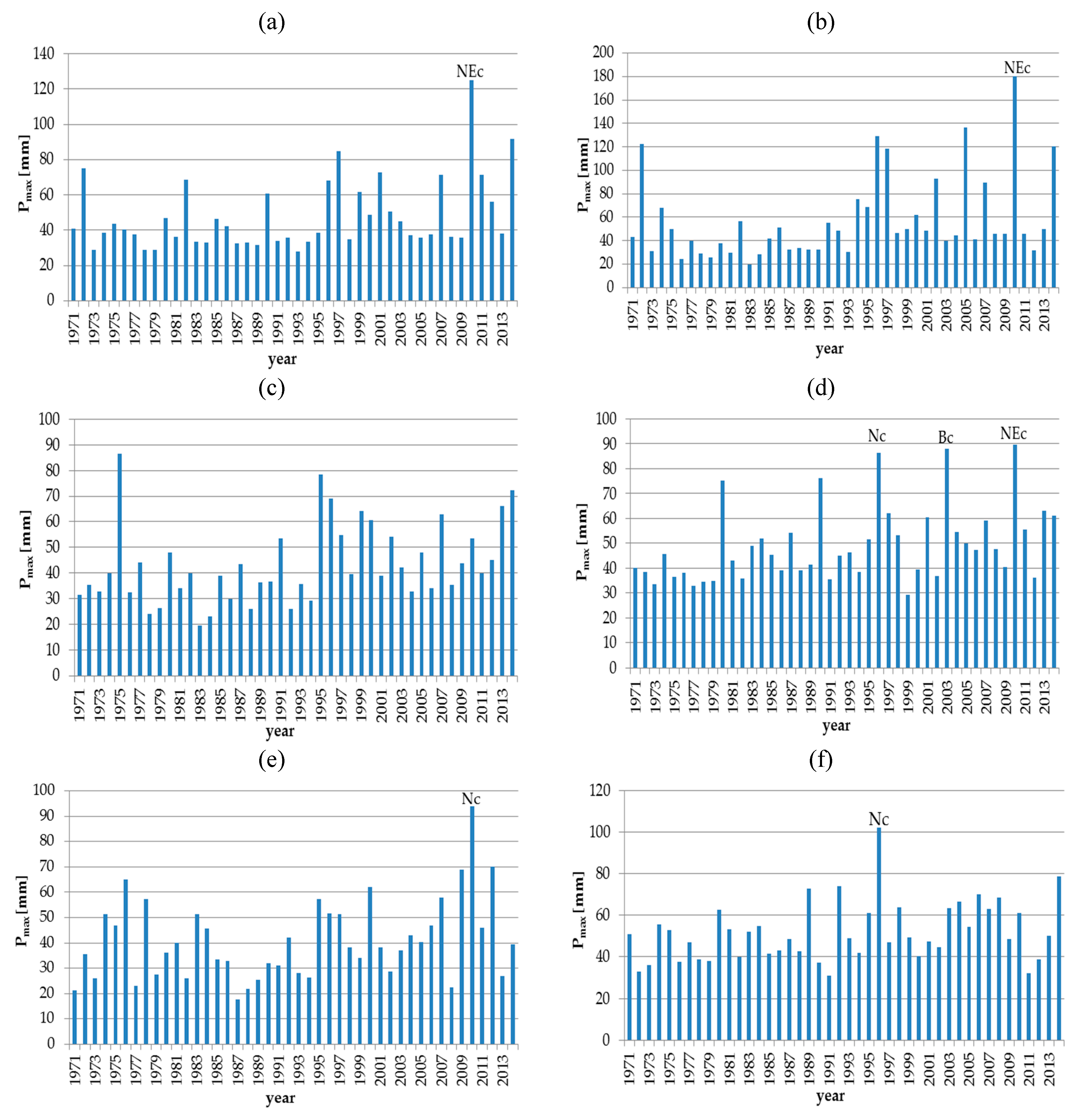
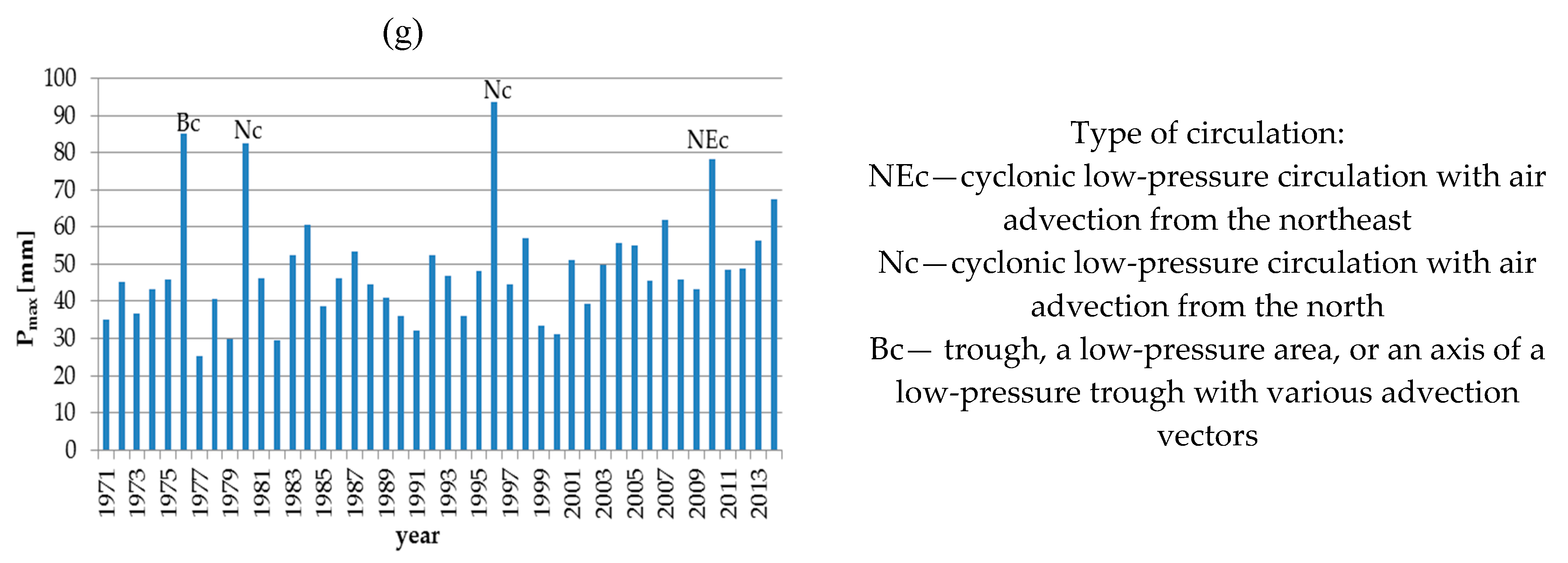
4.1. Preliminary Analysis of the Annual Maximum Precipitation

Table 1. The characteristics of the annual maximum precipitation in the analyzed period.

Station	LPmax	MPmax	HPmax	s	Cs	A
	mm	mm	mm	mm	-	-
Wisła-Malinka	34.5	64.8	151.4	27.2	0.42	1.3
Istebna-Stecówka	26.9	56.9	133.6	22.2	0.39	1.6
Goczałkowice	23.0	45.4	149.7	22.6	0.50	2.7
Rudzica	21.7	47.4	108.7	16.1	0.34	1.8
Szczyrk	36.3	70.3	213.0	32.3	0.46	2.3
Bielsko-Biała	24.9	55.5	162.7	26.7	0.48	2.4
Piwoń	17.5	36.9	96.8	13.3	0.36	2.2
Wolbrom	18.6	41.3	82.3	14.8	0.36	0.9
Żabnica	22.5	57.8	192.0	31.8	0.55	2.4
Korbielów	29.7	52.2	106.1	17.0	0.33	1.4
Rajcza	27.7	47.9	124.8	19.8	0.41	1.8
Maków Podhalański	21.0	54.5	190.8	30.2	0.55	2.4
Koszarawa	30.3	52.5	90.6	15.9	0.30	0.6
Zawoja	28.8	58.1	138.0	24.1	0.42	1.5
Gierałtowice	26.9	50.1	133.4	21.4	0.43	2.0
Wadowice	24.0	46.7	118.4	18.3	0.39	1.8
Kocierz Moszczanicki	19.9	57.0	180.4	34.9	0.61	1.8
Stróża	22.4	46.3	129.5	18.4	0.40	2.3
Radziszów	20.7	42.9	82.4	15.1	0.35	1.1
Kraków Balice	17.8	40.0	87.4	13.9	0.35	1.0
Węglówka	24.9	53.6	112.1	18.4	0.34	1.1
Książ Wielki	19.4	43.4	86.4	15.4	0.35	0.9
Kazimierza Mała	21.0	34.3	71.1	10.7	0.31	1.2
Kraków UJ	17.5	39.0	79.0	14.8	0.38	1.0
Borzęcin	20.6	43.6	125.2	20.4	0.47	1.9
Rozdziele	21.2	50.4	126.1	20.6	0.41	2.0
Szaflary	23.2	45.3	103.2	17.0	0.38	1.7
Kasprowy Wierch	36.4	81.2	232.0	36.6	0.45	1.9
Szczawne	26.2	47.7	77.8	12.0	0.25	0.4
Temeszów	21.3	44.8	88.5	14.0	0.31	1.1
Wisłok Wielki	29.3	48.9	89.7	15.0	0.31	1.3
Nowy Sącz	25.4	45.7	82.6	14.8	0.32	0.9
Bartków	17.6	37.0	70.3	13.5	0.37	0.8
Kielce	17.0	38.9	155.2	21.4	0.55	3.8
Małogoszcz	19.0	36.8	80.4	13.4	0.36	1.5
Sędziszów	16.6	37.7	75.3	13.8	0.37	0.8
Raków	19.6	36.1	114.2	16.5	0.46	2.6
Szydłów	18.8	35.8	79.5	11.8	0.33	1.3
Radomyśl Wielki	17.8	40.5	93.9	15.7	0.39	1.1
Dąbrowa Tarnowska	23.1	43.3	152.7	19.1	0.44	4.2
Ropczyce	21.6	49.0	98.4	14.9	0.30	0.9
Brzeziny	22.3	43.8	95.4	17.0	0.39	1.2
Szerzyny	28.5	49.1	85.2	13.1	0.27	0.4
Wysowa	21.9	48.2	84.5	15.1	0.31	0.5
Jaśliska	24.0	48.3	105.7	14.9	0.31	1.7
Barwinek	23.8	43.9	78.4	11.6	0.26	1.2
Staszów	18.3	36.3	71.6	11.9	0.33	0.7
Lutowiska	25.3	49.7	94.7	15.3	0.31	0.9
Teleśnica	21.0	52.0	111.3	18.7	0.36	0.9
Cisna	30.9	51.8	102.0	14.1	0.27	1.2
Komańcza	25.1	48.5	93.5	14.6	0.30	1.3

LP_max—minimum values of precipitation, MP_max—mean values of precipitation, HP_max—maximum values of precipitation, C_s—coefficient of variation, s—standard deviation, A—the coefficient of skewness

presents the values of the descriptive statistics for the annual maximum precipitation time series for all the stations.

Based on Table 1, it is concluded that the coefficient of variation C_s mostly remained below 40%, which indicates an average variability of P_max in the time series. The lowest value of C_s was for Szczawne (25%) and the highest for Kocierz Moszczanicki (61%). The values of the coefficient of skewness (A) were above zero in each time-series, which proved the right-sided asymmetry of the empirical distributions of the variates. This is due to the fact that for the analyzed time-series the majority of the series means observations are lower than the median values.

4.2. Analysis of Trends in the Observed Series

The observation series of the maximum annual daily precipitation were analyzed for significant monotonic trends with the Mann-Kendall tests. The findings are presented in Figure 2. Figure 3 presents a time series of the annual maxima daily precipitation for rainfall stations with a significant trend.

A significant (only positive) trend indicating long-term change at the assumed significance level was found for seven out of 51 rainfall stations (that is, Rajcza, Radziszów, Książ Wielki, Wisłok Wielki, Radomyśl Wielki, Cisna, and Komańcza). Figure 3 presents the time series of the annual maxima daily precipitation for rainfall stations with significant trend along with the indication of generation mechanisms for the greatest values. The stations with a significant trend were located in the mountainous (Rajcza, Wisłok Wielki, Cisna, Komańcza) and highland (Radziszów, KsiążWielki, Radomyśl Wielki) parts of the Upper Vistula Basin. Also, it should be mentioned that Wisłok Wielki, Cisna, Komańcza, and Radomyśl Wielki are placed in the Bieszczady, which are located in the mid-mountain part of the Carpathian. As can be seen in Figure 3d–g, most of the highest observations for these stations were for the years 1997 and 2010. Such years in Poland were characterized by extremely high precipitation, with the highest precipitation being observed in the south-east part of Poland. Such high precipitation was caused by incoming moist air masses from Ukraine and the Great Hungarian Plain. The other rainfall stations showed no significant trends in the observation series. This is consistent with studies on the behavior of the highest total daily precipitation in Southern Poland that reported irregular fluctuations rather than a trend [58]. Niedźwiedź et al. [59], who also investigated the area of Southern Poland, obtained similar results usually indicating a lack of significant trends. Our findings are also consistent with trend results for maximum flows in the Upper Vistula Basin. As shown by studies conducted in this region over the past decades [60], these flows were characterized by the lack of any trend in their values. The relationship between the maximum annual daily precipitation and the maximum flows results from the physiographic characteristics of the Upper Vistula Basin that affect the rainfall-runoff transformation [61].

4.3. Identification of Empirical Distributions with Kernel Estimators

The statistical analysis was expanded by using kernel density estimators to evaluate the distribution of the maximum annual daily precipitation for the stations showing significant trends in the observation series. Results are presented in Figure 4.

The kernel estimation of the density function for the maximum annual daily precipitation revealed a multimodal nature of the density function for all cases exhibiting trends. This indicates a subpopulation within the investigated observation series, thus suggesting a change in the weather mechanisms that trigger intense rainfall, such as high content of water vapor, temperature differences between the incoming and lingering air masses, time of low pressure persistence over the given area, thermodynamic equilibrium of the atmosphere and local conditions [62]. This was also confirmed by significant trends of P_max for the selected observation series. For six stations where multimodality was demonstrated on the basis of the density kernel analysis—Figure 4 (Rajcza, Radziszów, Wisłok Wielki, Radomysl Wielki, Cisna and Komańcza)—the circulation situation was analyzed, see Figure 3. Details on the circulation situation analysis were presented by Młyński et al. [63]. In 45.8% of the highest P_max values, the situation corresponded to Nc (cyclonic low-pressure circulation with air advection from the north), NEc (cyclonic low-pressure circulation with air advection from the northeast) and Bc (trough, a low-pressure area, or an axis of a low-pressure trough with various advection vectors), but 37.5% of them were caused by Nc and NEc circulations. In the case of the rest of the P_max values (smaller than the value of the highest values), they were caused by Cc (central cyclonic, center of low pressure —37% of all rainfall for the analyzed stations). The presented results show a different genesis for the formation of the maximum rainfall since the highest values are in relation to the other values. Additionally, it must be emphasized that extreme values are not necessarily clustered in recent years, and it cannot be said that the increasing trend could be attributed only to the occurrence of these extremes (the trends should also be attributed to an increase in the mid-range values).

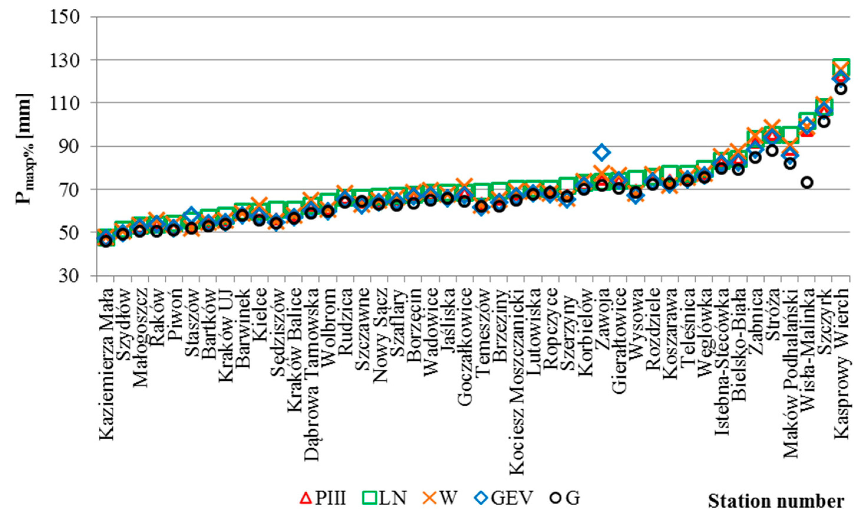
4.4. Determination of the Maximum Annual Daily Precipitation with Specific Probability of Exceedance

The maximum annual daily precipitation with a specific probability of exceedance was calculated using four distributions. The calculations were carried out for the rainfall stations where the observation series did not show a significant trend. The Kolmogorov–Smirnov test for significance level α = 0.05 confirmed the consistency of the analyzed theoretical distributions with the empirical distributions of the random variables in all tested cases. Figure 5 presents the values of P_max10% determined using the analyzed statistical distributions. Figure 6 presents the example P_maxp% results obtained by using the theoretical distribution for Wisła-Malinka station.

The values of P_max10% and especially, quantiles of a smaller probability of exceedance are commonly used in hydrological engineering. This precipitation is considered reliable for designing rainwater draining systems in rural areas. Our calculations revealed that the highest values of P_max10% were most commonly obtained from the log-normal distribution (58% of all rainfall stations). The lowest values of P_max10% were usually derived from the Gumbel’s distribution (84% of all rainfall stations). The highest P_max10% quantile values obtained using the log-normal distribution are justified by the properties of such a model. In fact, the log-normal is one of the heavy-tailed distributions, which means that with the same order of the upper quantile, e.g., probability p ≤ 0.2, it generates much higher quantile values than other probability distributions [64]. The GEV distribution shows similar properties; hence, it also yields high values for low quantiles, such as for the Zawoja station. Moreover, it is clear that quantile estimates of maximum precipitation for lower frequency have a higher difference between distributions than for higher frequency. Therefore, it is important to apply the goodness-of-fit metrics that are more sensitive to differences in quantiles with a low frequency (heavy-tailed distribution).

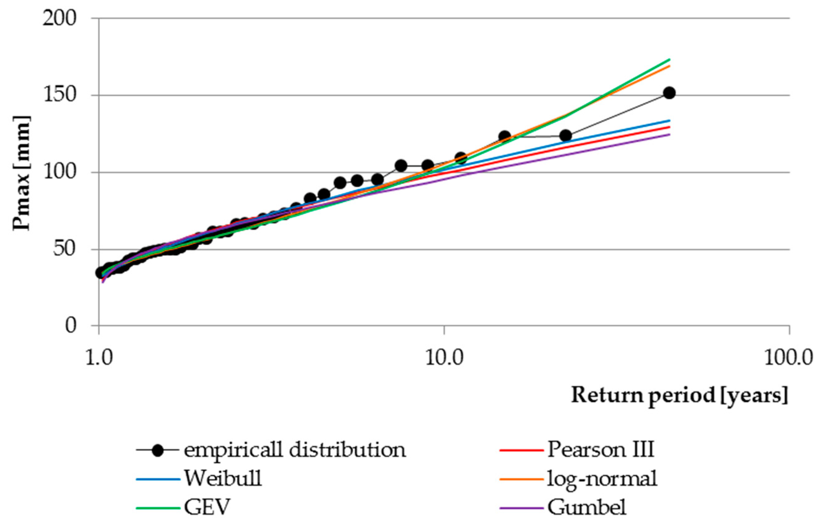
4.5. Selection of the Best Fit between the Theoretical and Empirical Distribution of Random Variables

The analysis of fit between the theoretical and empirical distributions of the maximum annual daily precipitation was based on RMSE, R², and the adapted PWRMSE goodness-of-fit metrics. The results of these calculations are shown in

Table 2. Values of the analyzed goodness-of-fit measures matching the theoretical distributions.

Station Number	Station	The Best Adjusted Distribution (Goodness-of-Fit Measures Value)
		PWRMSE	RMSE	R2
1	Wisła-Malinka	W (5.307)	W (4.583)	W (0.985)
2	Istebna-Stecówka	LN (4.896)	LN (4.019)	GEV (0.985)
3	Goczałkowice	GEV (8.237)	GEV (5.799)	GEV (0.971)
4	Rudzica	GEV (8.237)	GEV (8.237)	GEV (0.943)
5	Szczyrk	GEV (8.135)	GEV (6.253)	GEV (0.972)
6	Bielsko-Biała	GEV (10.625)	GEV (7.826)	GEV (0.951)
7	Piwoń	LN (4.181)	LN (3.322)	LN (0.939)
8	Wolbrom	PIII (1.789)	PIII (1.700)	G (0.990)
9	Żabnica	GEV (9.718)	GEV (7.082)	GEV (0.970)
10	Korbielów	GEV (13.346)	GEV (11.562)	GEV (0.987)
11	Maków Podhalański	LN (6.391)	LN (5.189)	LN (0.973)
12	Koszarawa	PIII (2.301)	PIII (2.179)	GEV (0.985)
13	Zawoja	GEV (3.669)	GEV (3.258)	W (0.990)
14	Gierałtowice	GEV (3.769)	GEV (3.078)	GEV (0.991)
15	Wadowice	LN (4.635)	LN (3.836)	GEV (0.970)
16	Kociesz Moszczanicki	LN (5.155)	LN (4.078)	LN (0.952)
17	Stróża	LN (3.191)	LN (2.833)	LN (0.971)
18	Kraków Balice	PIII (2.807)	PIII (2.432)	GEV (0.977)
19	Węglówka	LN (1.942)	LN (1.879)	GEV (0.993)
20	Kaziemierza Mała	LN (1.367)	LN (1.210)	GEV (0.992)
21	Kraków UJ	GEV (2.498)	GEV (2.251)	GEV (0.982)
22	Borzęcin	GEV (4.251)	GEV (3.259)	GEV (0.991)
23	Rozdziele	LN (6.815)	LN (5.702)	LN (0.929)
24	Szaflary	LN (2.723)	LN (2.458)	LN (0.981)
25	Kasprowy Wierch	LN (7.161)	LN (5.561)	GEV (0.979)
26	Szczawne	PIII (1.213)	PIII (1.241)	GEV (0.994)
27	Temeszów	PIII (2.647)	PIII (2.414)	G (0.974)
28	Nowy Sącz	PIII (2.247)	PIII (2.029)	PIII (0.989)
29	Bartków	PIII (2.564)	PIII (2.280)	W (0.978)
30	Kielce	LN (14.507)	LN (9.344)	GEV (0.853)
31	Małogoszcz	LN (3.002)	LN (2.495)	GEV (0.972)
32	Sędziszów	G (20.318)	G (19.112)	GEV (0.989)
33	Raków	GEV (4.738)	GEV (3.528)	GEV (0.964)
34	Szydłów	LN (1.905)	LN (1.668)	GEV (0.981)
35	Dąbrowa Tarnowska	GEV (2.552)	GEV (2.186)	GEV (0.747)
36	Ropczyce	G (2.752)	G (2.502)	G (0.973)
37	Brzeziny	GEV (3.080)	GEV (2.700)	GEV (0.984)
38	Szerzyny	W (2.075)	W (2.028)	GEV (0.979)
39	Wysowa	W (1.976)	W (2.196)	W (0.988)
40	Jaśliska	LN (3.575)	LN (3.267)	LN (0.953)
41	Barwinek	LN (2.058)	LN (2.012)	LN (0.971)
42	Staszów	G (1.669)	G (1.591)	W (0.985)
43	Lutowiska	LN (1.482)	LN (1.432)	GEV (0.995)
44	Teleśnica	LN (2.758)	LN (2.601)	GEV (0.984)

PWRMSE—peak-weighted root mean square error, RMSE—the root mean square error, R² —coefficient of determination, PIII—Pearson’s type III distribution, W—Weibull distribution, GEV—generalized extreme value distribution, G—Gumbel distribution.

.

According to the PWRMSE goodness-of-fit metrics, the values presented in Table 2 identified the log-normal distribution as the most suitable probability distribution function for estimating the quantiles of P_maxp%. This was confirmed for 41% of all rainfall stations. The other most suitable distributions according to this goodness-of-fit measures were GEV (29% of all rainfall stations), Pearson’s type III (16%), and Weibull’s (7%) and Gumbel’s (7%). The RMSE goodness-of-fit metrics yielded the same pattern of results. Additionally, both the PWRMSE and the RMSE goodness-of-fit metrics indicated the same best-fitting theoretical distributions of the probability functions for all the analyzed stations. The value of PWRMSE was nearly always higher than that of RMSE (on average by 15%). This is due to the higher weight attributed to values above the average in the PWRMSE goodness-of-fit metrics, whereas, for the RMSE goodness-of-fit metrics, every value has the same weight. The values of the R² goodness-of-fit metrics revealed a very strong determination between the empirical data and the values derived from statistical distributions. The coefficient of determination R² identified GEV as the best-fitting distribution type (62% of all rainfall stations), followed by log-normal (18%), and Weibull’s (11%), Gumbel’s (7%), and Pearson’s type III distributions (2%).

Our study identified the log-normal and GEV functions (the same family of distributions) as the recommended statistical distributions for the determination of the P_maxp% quantiles. This is evidenced by the results of inference carried out using PWRMSE for assessing the quality of the statistical distributions. In fact, this goodness-of-fit measure indicated the best fit of these distributions in the largest number of cases. While studies on the best-fit probability distributions for the estimation of P_maxp% quantiles have not been conducted on a wider scale neither in Poland nor in Central Europe and there is no detailed research in this study area in southern Poland, a report by Cebulska [65] also indicated the log-normal and Weibull’s distributions as the best for the Orava-Nowy Targ Basin (the Carpathian part of the Upper Vistula Basin). Another study [66] suggested Weibull’s and log-gamma distribution as the best-fitting ones for central Poland. The research carried out by Wdowikowski et al. [14] confirmed the generalized exponential distribution as the best measure for estimating P_maxp% in the Upper Odra Basin. Villarini [67] claimed the GEV function to be the best distribution to estimate the maximum annual daily precipitation with a specific probability of exceedance in the countries of Central Europe due to its upper tail. Despite such studies, it should be noted that the form of the probability distributions (and particularly their parameters) are closely related to the areas (physical, geographical, and meteorological characteristics affecting the precipitation) for which the maximum daily precipitation with a specific probability of exceedance is determined [28].

5. Conclusions

Our calculations showed a lack of significant trends in the observation series of the investigated random variables for a majority of rainfall stations in the Upper Vistula Basin (44 out of 51). The multimodality of the empirical density function for the rainfall stations with significant trends confirmed the change in meteorological mechanisms in the surveyed multi-year period that affected the maximum daily precipitation in the Upper Vistula Basin. We found that the peak-weighted root mean square error (PWRMSE) goodness-of-fit metrics, commonly used in the quality assessment of rainfall-runoff models, may be used for identifying the best-fit statistical distributions. This was also confirmed by the root mean square error (RMSE) goodness-of-fit metrics. We also identified the log-normal and generalized extreme value GEV distributions as suitable for calculating the maximum daily precipitation with a specific probability of exceedance in the catchments of the Upper Vistula Basin (according to the PWRMSE goodness-of-fit metrics, the log-normal was the best for 41% and the GEV for 29% of all the stations; according to the RMSE goodness-of-fit metrics, consistent results were found; according to coefficient of determination R², the GEV was optimal for 62% and the log-normal for 18% of all the stations). Since the obtained results from PWRMSE goodness-of-fit metrics, with regard to the best-fitted distribution, were similar to RMSE and R², it was concluded that the analyzed methods can be used interchangeably. In addition, it was concluded that PWRMSE can be used as the goodness-of-fit metric instead of other goodness-of-fit measures.

References

1. Schmocker-Fackel, P.; Naef, F. More frequent flooding? Changes in flood frequency in Swicerland since 1850. J. Hydrol. 2010, 381, 1–8. [Google Scholar] [CrossRef]
2. Wałęga, A.; Kaczor, G.; Stęplewski, B. The Role of Local Precipitation Models in Designing Rainwater Drainage Systems in Urban Areas: A Case Study in Krakow, Poland. Pol. J. Environ. Stud. 2016, 25, 2139–2149. [Google Scholar] [CrossRef]
3. Chmielowski, K.; Bugajski, P.M.; Kaczor, G. Effects of precipitation on the amount and quality of raw sewage entering a sewage treatment plant in Wodzisław Śląski. J. Water Land Dev. 2017, 34, 85–93. [Google Scholar] [CrossRef] [Green Version]
4. Coumou, D.; Rahmstorf, S.A. decade of weather extremes. Nat. Clim. Chang. 2012, 2, 491–496. [Google Scholar] [CrossRef]
5. Min, K.S.; Zhang, X.; Zwiers, F.W.; Hegerl, G.C. Human contribution to more-intense precipitation extremes. Nature 2011, 470, 378–381. [Google Scholar] [CrossRef] [PubMed]
6. Tye, M.R.; Colley, D. A spatial model to examine rainfall extremes in Colorado’s Front Range. J. Hydrol. 2015, 530, 15–23. [Google Scholar] [CrossRef]
7. Singh, B.; Rajpurohit, D.; Vasishth, A.; Singh, J. Probability analysis for estimation of annual one day maximum rainfall of Jhalarapatan Area of Rajasthan. India Plant Arch. 2012, 12, 1093–1100. [Google Scholar]
8. Papalexiou, S.M.; Koutsoyiannis, D.; Makropoulos, C. How extreme is extreme. An assessment of daily distribution tails. Hydrol. Earth Syst. Sci. 2013, 17, 851–862. [Google Scholar] [CrossRef]
9. Salinas, J.L.; Castellarin, A.; Kohnová, S.; Kjeldsen, T.R. Regional parent flood frequency distributions in Europe—Part 2: Climate and scale controls. Hydrol. Earth Syst. Sci. 2014, 18, 4391–4401. [Google Scholar] [CrossRef]
10. Amin, M.T.; Rizwan, M.; Alazba, A.A. Abest fit probability distribution for the estimation of rainfall in northen regions of Pakistan. Open Life Sci. 2016, 11, 432–440. [Google Scholar]
11. Sun, H.; Wang, G.; Li, X.; Chen, J.; Su, B.; Jiang, T. Regional frequency analysis of observed sub-daily rainfall maxima over eastern China. Adv. Atmos. Sci. 2017, 34, 209–225. [Google Scholar] [CrossRef]
12. Douka, M.; Karacostas, T.S.; Katragkou, E.; Anagnostolpoulou, C. Annual and seasonal extreme precipitation probability distributions at Thessaloniki based upon hourly values. In Perspectives on Atmospheric Sciences; Karacostas, T., Bais, A., Nastos, P., Eds.; Springer Atmospheric Sciences; Springer: Cham, Switzerland, 2017. [Google Scholar]
13. Boudrissa, N.; Cheraitia, H.; Haliami, L. Modelling maximum daily yearly rainfall in northern Algeria using generalized extreme value distributions from 1936 to 2009. Meteorol. Appl. 2017, 24, 114–119. [Google Scholar] [CrossRef] [Green Version]
14. Wdowikowski, M.; Kaźmierczak, B.; Levinka, O. Maximum daily rainfall analysis at selected meteorological stations in the upper Lusatian Neisse River basin. Meteorol. Hydrol. Water Manag. 2016, 4, 53–63. [Google Scholar] [CrossRef] [Green Version]
15. Koutsoyiannis, D. Statistics of extremes and estimation of extreme rainfall: I. Theoretical investigation. Hydrol. Sci. J. 2004, 49, 575–590. [Google Scholar] [CrossRef]
16. Koutsoyiannis, D. Statistics of extremes and estimation of extreme rainfall: II. Empirical investigation of long rainfall records. Hydrol. Sci. J. 2004, 49, 591–610. [Google Scholar] [CrossRef]
17. Haddad, K.; Rahman, A. Selection of the best fit flood frequency distribution and parameter estimation procedure: A case study for Tasmania in Australia. Stoch. Environ. Res. Risk Assess. 2011, 25, 415–428. [Google Scholar] [CrossRef]
18. Laio, F.; Di Baldassarre, G.; Montanari, A. Model selection techniques for the frequency analysis of hydrological extremes. Water Resour. Res. 2008, 45. [Google Scholar] [CrossRef]
19. Sun, X.; Lall, U. Spatially coherent trends of annual maximum daily precipitation in the United States. Geophys. Res. Lett. 2015, 42, 9781–9789. [Google Scholar] [CrossRef]
20. Delignette-Muller, M.L.; Dutang, C. An R Package for fitting distributions. J. Stat. Softw. 2015, 64, 1–34. [Google Scholar] [CrossRef]
21. Wałęga, A. The importance of the objective functions and flexibility on calibration of parameters of Clark instantaneous unit hydrograph. Geomat. Landmanag. Landsc. 2014, 2, 75–85. [Google Scholar] [CrossRef]
22. Wałęga, A.; Książek, L. Influence of rainfall data on the uncertainty of flood simulation. Soil Water Res. 2016, 11, 277–284. [Google Scholar] [CrossRef] [Green Version]
23. Wałęga, A.; Młyński, D.; Bogdał, A.; Kowalik, T. Analysis of the course and frequency of high water stages in selected catchments of the Upper Vistula basin in the south of Poland. Water 2016, 8, 394. [Google Scholar] [CrossRef]
24. Wałęga, A.; Młyński, D.; Wachulec, K. The use of the asymptotic functions for determing empirical values of CN parameter in selected catchments of variable land cover. Studia Geotechnica et Mechanica 2018, 39, 111–120. [Google Scholar] [CrossRef]
25. Amirataee, B.; Montaseri, M.; Rezaei, H. Assessment of goodness of fit methods in determing the best regional probability distribution of rainfall data. Int. J. Eng. 2014, 27, 1537–1546. [Google Scholar]
26. Ba, I.; Ashkar, F. Discrimination between a group of three-parameter distributions for hydro-meteorological frequency modeling. Can. J. Civ. Eng. 2018, 45, 351–365. [Google Scholar] [CrossRef]
27. Hinkle, D.E.; Wiersma, W.; Jurs, S.G. Applied Statistics for the Behavioral Sciences; Houghton Mifflin: Boston, MA, USA, 2003. [Google Scholar]
28. Alam, M.A.; Emuro, K.; Farnham, C.; Yuan, J. Best-fit probability distributions and return periods for maximum monthly rainfall in Bangladesh. Climate 2018, 6, 9. [Google Scholar] [CrossRef]
29. Kumar, A. Prediction of annual maximum daily rainfall of Ranichauri (Tehri Garhwal) based on probability analysis. Ind. J. Soil Conserv. 2000, 28, 178–180. [Google Scholar]
30. Lee, C. Application of rainfall frequency analysis on studying rainfall distribution characteristics of Chia-Nan plain area in Southern Taiwan. Crop Environ. Bioinf. 2005, 2, 31–38. [Google Scholar]
31. Kundzewicz, Z.W.; Stoffel, M.; Niedźwiedź, T.; Wyżga, B. Flood Risk in the Upper Vistula Basin; Springer: Cham, Switzerland, 2016. [Google Scholar]
32. Tabari, H.; Marofi, S.; Aeini, A.; Talaee, P.H.; Mohammadi, K. Trend analysis of reference evapotranspiration in the western half of Iran. Agric. For. Meteorol. 2011, 151, 128–136. [Google Scholar] [CrossRef]
33. Rutkowska, A.; Ptak, M. On certain stationary tests for hydrological series. Studia Geotechnica et Mechanica 2012, 4, 51–63. [Google Scholar] [CrossRef]
34. Banasik, K.; Hejduk, L. Long term changes in runoff from a small agricultural catchment. Soil Water Res. 2012, 7, 64–72. [Google Scholar] [CrossRef]
35. Jeneiová, K.; Kohnová, S.; Sabo, M. Detecting trends in the annual maximum discharges in the Vah River Basin, Slovakia. Acta Silv. Lign. Hung. 2014, 10, 133–144. [Google Scholar] [CrossRef]
36. Blain, G.C. The influence of nonlinear trends on the power of the trend-free pre-whitening approach. Acta Scientarum Agron. 2015, 37, 21–28. [Google Scholar] [CrossRef]
37. Mann, H.B. Non-parametric tests against trend. Econometrica 1945, 13, 245–259. [Google Scholar] [CrossRef]
38. Kendall, M.G. Rank Correlation Methods; Charles Griffin: London, UK, 1975. [Google Scholar]
39. Hamed, K.H.; Rahman, A. A modified Mann-Kendall trend test for autocorrelated data. J. Hydrol. 1998, 204, 219–246. [Google Scholar] [CrossRef]
40. Haghighatjou, P.; Akhoond-Ali, A.M.; Nazemosadat, M.J. Nonparametric kernel estimation of annual precipitation over Iran. Theor. Appl. Climatol. 2013, 112, 193–200. [Google Scholar] [CrossRef]
41. Krakauer, N.Y.; Pradhanang, S.M.; Panthi, J.; Lakhankar, T.; Jha, A.J. Probabilistic precipitation estimation with a satellite product. Climate 2015, 3, 329–348. [Google Scholar] [CrossRef]
42. Mosthaf, T.; Bárdossy, A. Regionalizing nonparametric models of precipitation amounts on different temporal scales. Hydrol. Earth Syst. Sci. 2017, 21, 2463–2481. [Google Scholar] [CrossRef]
43. Peng, J.; Zhao, S.; Liu, X.; Tian, L. Identifying the urban-rural fringe using wavelet transform and kernel density estimation: A case study in Beijing City, China. Environ. Model. Softw. 2016, 83, 286–302. [Google Scholar] [CrossRef]
44. Pathiraja, S.; Moradkhani, H.; Marshall, L.; Sharma, A.; Geenens, G. Data-driven model uncertainty estimation in hydrologic data assimilation. Water Resour. Res. 2018, 54, 1252–1280. [Google Scholar] [CrossRef]
45. Silverman, B.W. Density Estimation for Statistics and Data Analysis; Chapman and Hall: London, UK, 1986. [Google Scholar]
46. Sivakumar, B. Chaos in Hydrology: Bridging Determinism and Stochasticity; Springer: Sidney, BC, Canada, 2016. [Google Scholar]
47. Węglarczyk, S. Statistics in Environmental Engineering; Cracow University of Technology Publishing House: Kraków, Poland, 2010. (In Polish) [Google Scholar]
48. Młyński, D. Analysis of the form of probability distribution to calculate flood frequency in selected mountain river. Episteme 2016, 1, 399–411. (In Polish) [Google Scholar]
49. Strupczewski, W.G.; Singh, V.P.; Węglarczyk, S. Asymptotic bias of estimation methods caused by the assumption of false probability distribution. J. Hydrol. 2002, 258, 122–148. [Google Scholar] [CrossRef]
50. Strupczewski, W.G.; Kochanek, K.; Bogdanowicz, E.; Markiewicz, I. The accuracy of skewness coefficient and flood quantiles estimated by means of weighted function method for Pearson type 3 distribution function. In Hydrologia w i Inżynierii i Ochronie Środowiska; Więzik, W., Hejduk, L., Eds.; Publ. PAN: Warsaw, Poland, 2018. (In Polish) [Google Scholar]
51. McNeil, A.J. Estimating the tail of loss severity distributing using extreme value theory. ASTIN Bull. 1997, 27, 117–137. [Google Scholar] [CrossRef]
52. Degeling, K.; IJzerman, M.J.; Koopman, M.; Koffijberg, H. Accounting for parameter uncertainty in the definition of parametric distributions used to describe individual patient variation in health economic models. BMC Med. Res. Methodol. 2017, 17, 170. [Google Scholar] [CrossRef] [Green Version]
53. Zeng, X.; Wang, D.; Wu, J. Comparisons of methods of goodness of fit tests in hydrologic analysis. In Emerging, Economies, Risk and Development and Intelligent Technology; Huang, C., Lyhyaoui, A., Zhai, G., Benhayoun, N., Eds.; Taylor: London, UK, 2015. [Google Scholar]
54. Krause, P.; Boyle, D.P.; Base, F. Comparrison of different efficiency criteria for hydrological model assessment. Adv. Geosci. 2005, 5, 89–97. [Google Scholar] [CrossRef]
55. Chai, T.; Draxler, R.R. Root mean square error (RMSE) or mean absolute error (MAE)?—Arguments against avoiding RMSE in the literature. Geosci. Model Dev. 2014, 7, 1247–1250. [Google Scholar] [CrossRef]
56. Bezak, N.; Brilly, M.; Šraj, M. Flood frequency analyses, statistical trends and seasonality analyses of discharge data: A case study of the Litija station on the Sava River. Flood Risk Manag. 2016, 9, 154–168. [Google Scholar] [CrossRef]
57. Wałęga, A. The importance of calibration parameters on the accuracy of the floods description in the Snyder’s model. J. Water Land Dev. 2016, 28, 19–25. [Google Scholar] [CrossRef] [Green Version]
58. Cebulska, M.; Twardosz, R. Temporal variability of maximum monthly precipitation totals in the Polish Western Carpathian Mts during the period 1951–2005. Prace Geograficzne 2012, 128, 123–134. (In Polish) [Google Scholar]
59. Niedźwiedź, T.; Łupikasza, E.; Pińskwar, I.; Kundzewicz, Z.W.; Stoffel, M.; Małarzewski, Ł. Climatological background of floods at the northern foothills of the Tatra Mountains. Theor. Appl. Climatol. 2014, 119, 273–284. [Google Scholar] [CrossRef]
60. Młyński, D.; Petroselli, A.; Wałęga, A. Flood frequency analysis by an event-based rainfall-runoff model in selected catchments of southern Poland. Soil Water Res. 2018, 13, 170–176. [Google Scholar] [Green Version]
61. Kundzewicz, Z.W.; Pińskwar, I.; Choryński, A.; Wyżga, B. Floods still pose a hazard. Aura 2017, 3, 3–9. (In Polish) [Google Scholar]
62. Buchert, L.; Cebulak, L.; Drwal-Tylmann, A.; Wojtczak-Gaglik, E.; Kilar, P.; Limanówka, D.; Łapińska, E.; Mizera, M.; Ogórek, S.; Pryc, P.; et al. Dangerous Meteorological Phenomenas—Part 1 (Spring–Summer); Instytut Meteorologii i Gospodarki Wodnej Państwowy Instytut Badawczy: Warszawa, Poland, 2013. (In Polish) [Google Scholar]
63. Młyński, D.; Cebulska, M.; Wałęga, A. Trends, variability, and seasonality of maximum annual daily precipitation in the upper Vistula basin, Poland. Atmosphere 2018, 9, 313. [Google Scholar] [CrossRef]
64. Kochanek, K.; Feluch, W. The estimation of flood quantiles of selected heavy-tailed distribution by means of the method of the generalized moments. Przegląd Geofizyczny 2016, 3–4, 171–172. (In Polish) [Google Scholar]
65. Cebulska, M. The long-term variability of maximum daily precipitations in the Kotlina Orawsko-Nowotarska (Orawa-Nowy Targ Valley) (1984–2013). Czasopismo Inżynierii Lądowej Środowiska i Architektury 2015, 32, 49–60. (In Polish) [Google Scholar]
66. Krężałek, K.; Szymczak, T.; Bąk, B. The annual maximum daily rainfall with different probabilities of exceedance in central Poland based on data from the multiannual period 1966–2010. Woda-Środowisko-Obszary Wiejskie 2013, 13, 77–90. (In Polish) [Google Scholar]
67. Villarini, G. Analyses of annual and seasonal maximum daily rainfall accumulations for Ukraine, Moldova, and Romania. Int. J. Climatol. 2012, 32, 2213–2226. [Google Scholar] [CrossRef]
Figure 1. The digital elevation model of Upper Vistula Basin and rainfall stations location (black markers) on the map of Poland.
Atmosphere 10 00043 g001
Figure 2. Results of the Z statistics for the Mann-Kendall test.
Atmosphere 10 00043 g002
Figure 3. Time series of Pmax for the rainfall stations in (a) Rajcza; (b) Radziszów; (c) Książ Wielki; (d) Wisłok Wielki (e) Radomyśl Wielki; (f) Cisna; (g) Komańcza with the indication of generation mechanisms for the greatest values.
Atmosphere 10 00043 g003aAtmosphere 10 00043 g003b
Figure 4. Estimated kernel density function of Pmax for the rainfall stations in (a) Rajcza; (b) Radziszów; (c) Książ Wielki; (d) Wisłok Wielki; (e) Radomyśl Wielki; (f) Cisna; (g) Komańcza.
Atmosphere 10 00043 g004
Figure 5. Values of Pmax10% determined for the rainfall stations using the analyzed statistical distributions.
Atmosphere 10 00043 g005
Figure 6. Results of Pmaxp% calculations for Wisła-Malinka.
Atmosphere 10 00043 g006