Article

A Study on Microscale Wind Simulations with a Coupled WRF–CFD Model in the Chongli Mountain Region of Hebei Province, China

1
College of Meteorology and Oceanography, National University of Defense Technology, Nanjing 211101, China
2
Hebei Province Meteorological Bureau, Shijiazhuang 050000, China
3
State Key Laboratory of Aerospace, Xi’an 710000, China
*
Author to whom correspondence should be addressed.
Atmosphere 2019, 10(12), 731; https://doi.org/10.3390/atmos10120731
Submission received: 30 October 2019 / Revised: 13 November 2019 / Accepted: 19 November 2019 / Published: 21 November 2019
(This article belongs to the Section Meteorology)

Abstract

:
To ensure successful hosting of the 2022 Olympic Winter Games, a comprehensive understanding of the wind field characteristics in the Chongli Mountain region is essential. The purpose of this research was to accurately simulate the microscale wind in the Chongli Mountain region. Coupling the Weather Research and Forecasting (WRF) model with a computational fluid dynamics (CFD) model is a method for simulating the microscale wind field over complex terrain. The performance of the WRF-CFD model in the Chongli Mountain region was enhanced from two aspects. First, as WRF offers multiple physical schemes, a sensitivity analysis was performed to evaluate which scheme provided the best boundary condition for CFD. Second, to solve the problem of terrain differences between the WRF and CFD models, an improved method capable of coupling these two models is proposed. The results show that these improvements can enhance the performance of the WRF-CFD model and produce a more accurate microscale simulation of the wind field in the Chongli Mountain region.

1. Introduction

One site of the 2022 Olympic Winter Games, to be held in China, is located in the Chongli Mountain region of Hebei Province. To successfully host the Olympic Winter Games, meteorological support for the playing fields should be ensured. A comprehensive understanding of the wind-field characteristics in the Chongli Mountain region is essential for ensuring the safety of outdoor matches, such as ski jumping, cross-country skiing, and alpine skiing. Traditionally, the distribution of a wind field over flat terrain can be acquired from observations. However, the structures of a wind field in mountainous terrain are quite complex, and the representativeness of observation data is limited in a small area. Therefore, numerical simulation is the only method that can describe the detailed distribution of the wind field in the Chongli Mountain region.
In fact, wind field simulation over complex terrain is an important topic for consideration in the atmospheric science field. Traditionally, mesoscale models, such as the Fifth-Generation Penn State/National Center for Atmospheric Research Mesoscale Model (MM5), Regional Atmospheric Modelling System (RAMS), and Weather Research and Forecasting (WRF), are important tools in predicting the wind field over complex terrain [1,2,3,4,5,6,7,8]. However, a terrain-following coordinate system and smoothing processes for terrain data are applied to deal with the complex terrain in most mesoscale models [9,10,11]. Therefore, great terrain differences exist between reality and the mesoscale models, and nearly no mesoscale model can work over extremely steep terrain. Some scholars applied WRF in the large eddy simulation (LES) mode to increase model resolution [12,13,14], but the low vertical resolution and the need for a smoothing process for terrain data still exist. Moreover, the computational cost of a WRF–LES simulation is relative high. Fortunately, the computational fluid dynamics (CFD) model can partially compensate for the shortcomings of the mesoscale model. First, CFD can simulate the wind field with higher spatial resolutions (a few meters to tens of meters) than those of the mesoscale models [15,16,17,18]. Moreover, most CFD models are based on the finite volume method, which can improve their ability to depict realistic terrain [19]. However, CFD has its shortcoming in coping with the boundary conditions, and usually uses a simple wind profile as the boundary condition in some research. The mesoscale model can be initialized using global-scale data, such as the National Centers for Environmental Prediction (NCEP) reanalysis data. Therefore, coupling the mesoscale models with the CFD models is one way of simulating the microscale wind field over complex terrain. In this coupled system, the mesoscale and CFD models are combined in an off-line way, and the boundary condition that drives the CFD simulation is taken from the outputs of the mesoscale model [20]. First, the wind field with low spatial resolution is simulated by the WRF model. Second, the WRF wind data are imposed on the boundary of the CFD model. Finally, a wind field with higher spatial resolution is simulated by the CFD model. The advantages of this system is that the mesoscale model can provide more realistic boundary conditions and CFD can provide a wind field simulation with much higher spatial resolution.
In recent years, a large amount of research on wind field simulation has been conducted by using the mesoscale and CFD coupled system. Zajaczkowski et al. [21] coupled the ALADIN (Aire Limite Adaptation dynamique Dveloppement InterNational) and CFD models to predict the microscale wind field over complex terrain. Lei Li et al. [22] coupled the RAMS and FLUENT software to study the influence of airport buildings on the wind field simulation. Miao et al. [23] coupled the WRF and CFD models to predict the atmospheric flow and dispersion in Beijing. Mohan et al. [24] and Bindu et al. [25] coupled various mesoscale models with CFD and found that WRF performed the best among the mesoscale models. Temel et al. [26] coupled WRF and OpenFOAM to simulate atmospheric flow over complex terrain and presented a new Planetary Boundary Layer (PBL) scheme that supports the coupling process. Carvalho et al. [27] used WRF and a CFD model, WAsP (Wind Atlas Analysis and Application Program), for wind field simulation over complex terrain. Bilal et al. [28] coupled WRF and WindSim to simulate wind field over complex terrain. Fang et al. [29] studied the wind energy resources based on WRF and Meteodyn-WT (version 3.9.5) coupled system.
This study aimed at enhancing the performance of a mesoscale and CFD coupled system in the Chongli Mountain region from two aspects using the WRF mesoscale model [30]. First, In the WRF-CFD model system, the outputs of the WRF simulation were imposed on the CFD boundaries. Therefore, the performance of the WRF could directly influence the accuracy of the microscale wind field simulation. However, WRF offers multiple physical parameterizations that can be combined in any way. Different physical schemes have different impacts on the wind field simulation. Therefore, a sensitivity analysis was performed to evaluate which scheme provided the best boundary conditions for the CFD model. Second, the coupling method between the WRF and CFD models plays an important role in the simulation of the wind field. However, the CFD model commonly uses a single wind profile as an entire boundary condition, which may not correctly describe the effects of realistic terrain on the upwind direction. Therefore, an improved method that couples the WRF and CFD models is proposed in this study.
This paper comprises five parts: Section 2 describes the study area, model setups, and sensitivity analysis methodology. Section 3 discusses the two aspects (physical schemes and coupling method) to improve the WRF-CFD model performance. The results and discussion are provided in Section 4, while Section 5 draws some conclusions.

2. Methodology

Here, the study area for this research and the WRF and CFD model setups are discussed.

2.1. Study Area

The study area is located in the Chongli Mountain region of Zhangjiakou City, China. China will hold the 2022 Olympic Winter Games, and the host cities are Beijing, Yanqing, and Zhangjiakou. The outdoor games will be held in the Chongli Mountain region, Zhangjiakou City. This area is located in the north of the Inner Mongolia grassland, with a total area of 2334 km2. The terrain here is complex, with the altitude ranging from 814 to 2174 m. Furthermore, the steep terrain strongly affects the atmospheric flow, so the wind field in this area is relatively complex.
To guarantee the safety of the game fields, the Hebei Province meteorological bureau placed several automatic meteorological stations (AMSs) in the Chongli Mountain region. These stations provide daily observation data of the temperature, pressure, humidity, and wind at a height of 10 m. The observation campaign was performed from 00:00 on 21 May 2018, to 00:00 on 24 May 2018 (Beijing Time). The temporal resolution of the observed data is 10 s, and the time interval of observations used for the numerical simulation validation is 9 min after data averaging.

2.2. WRF Model Setup

The WRF model was used to provide the boundary condition for the CFD in this research. It can give more accurate wind estimation than other models or sources [24,31]. The WRF–ARW model (version 3.9) was utilized in this research and is designed for meteorological research and numerical weather prediction. A fully compressible, non-hydrostatic dynamic framework is adopted in the ARW module. In recent years, WRF has been widely used in both academic research and industry [32,33,34]. Many studies show that WRF can simulate lower boundary conditions well over complex orography [35,36], which can help WRF to couple with CFD accurately.
The simulated domain of WRF is shown in Figure 1. In Figure 1a, the scopes of four nested domains (D1~D4) used in the wind simulation are depicted. The horizontal resolutions of D1, D2, D3, and D4 are 27, 9, 3, and 1 km, respectively. Each domain has 100 × 100 grid points in the south-north and east-west directions. The WRF model contains 33 sigma levels in the vertical, and the lowest 21 levels utilized to provide the boundary conditions for the CFD are below 2000 m. The timesteps of D1~D4 are 108, 36, 12, and 4 s, respectively. These above settings, shown in Table 1, can guarantee the operation stability of the WRF model. In Figure 1b, the topographic distribution of the innermost domain (D4) is depicted, and the red box represents the CFD domain.
CFD results depend on the WRF performance, which in turn is strongly depend on the re-analysis dataset used as the initial and lateral boundary conditions. Marques [37], Carvalho [38], et al. found that NCEP re-analysis data can give better initial conditions for WRF compared to other re-analysis data. Therefore, the WRF simulations were initialized using the NCEP re-analysis data (http://rda.ucar.edu/dataset-s/ds083.2) in this research. The data were generated by the Global Data Assimilation System, and as part of the initial field of the Global Forecast System.

2.3. CFD Model Setup

The CFD model used for the microscale wind simulation was FLUENT software, a commercial software commonly used in research and industrial fields. FLUENT contains the physical modeling capability needed to model turbulence, flow, and so on. It also offers high-performance computing which can help solve complex computational fluid dynamics simulations quickly and effectively. More details on FLUENT can be found at https://www.ansys.com/products/fluids/ansys-fluent. In recent years, FLUENT has been widely used in the meteorological field. Li [22,39,40,41], Cabezón [42], Wei [43], et al. studied the wind field simulation over complex terrain using FLUENT.
FLUENT is a finite-volume method code, supporting both RANS (Reynolds-Averaged Navier-Stokes) and LES turbulence models. Due to the high precision, and lower computational cost compared with LES, the RANS turbulence model, with realizable k-ε, was used in this study [39,40]. The governing equations of CFD are as follows:
u i ¯ t + u j ¯ u i ¯ x j = 1 ρ p ¯ x i + μ ρ 2 u i ¯ x i x j x j ( u i u j ¯ ) + f i ,
u i ¯ x i = 0 ,
T ¯ t + u i ¯ T ¯ x i = k 2 T ¯ x i 2 ,
where u i ¯ and u j ¯ represent the mean velocity, u i and u j represent the turbulent variation, ρ represents the air density, f i represents the buoyancy, and T ¯ represents the mean temperature. The second-order upwind scheme was utilized for the discretization of the governing equations, and the body-fitted hexahedral grid system was used in the CFD domain. Moreover, the boundary condition of the ground in the CFD domain was set as “Wall”, the inlet boundary as “Velocity Inlet”, the outlet boundary as “Outflow”, and the other boundaries were set as “Symmetry”.
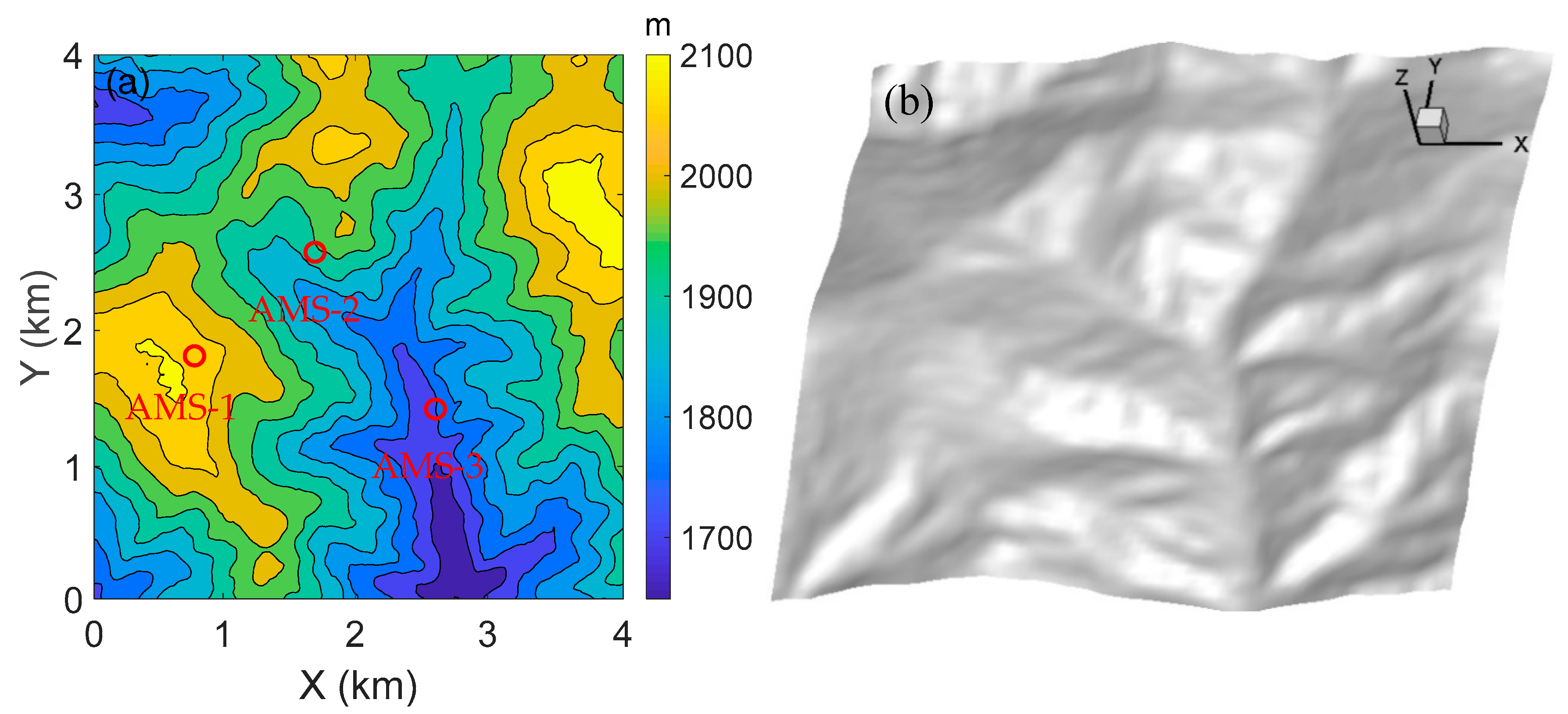
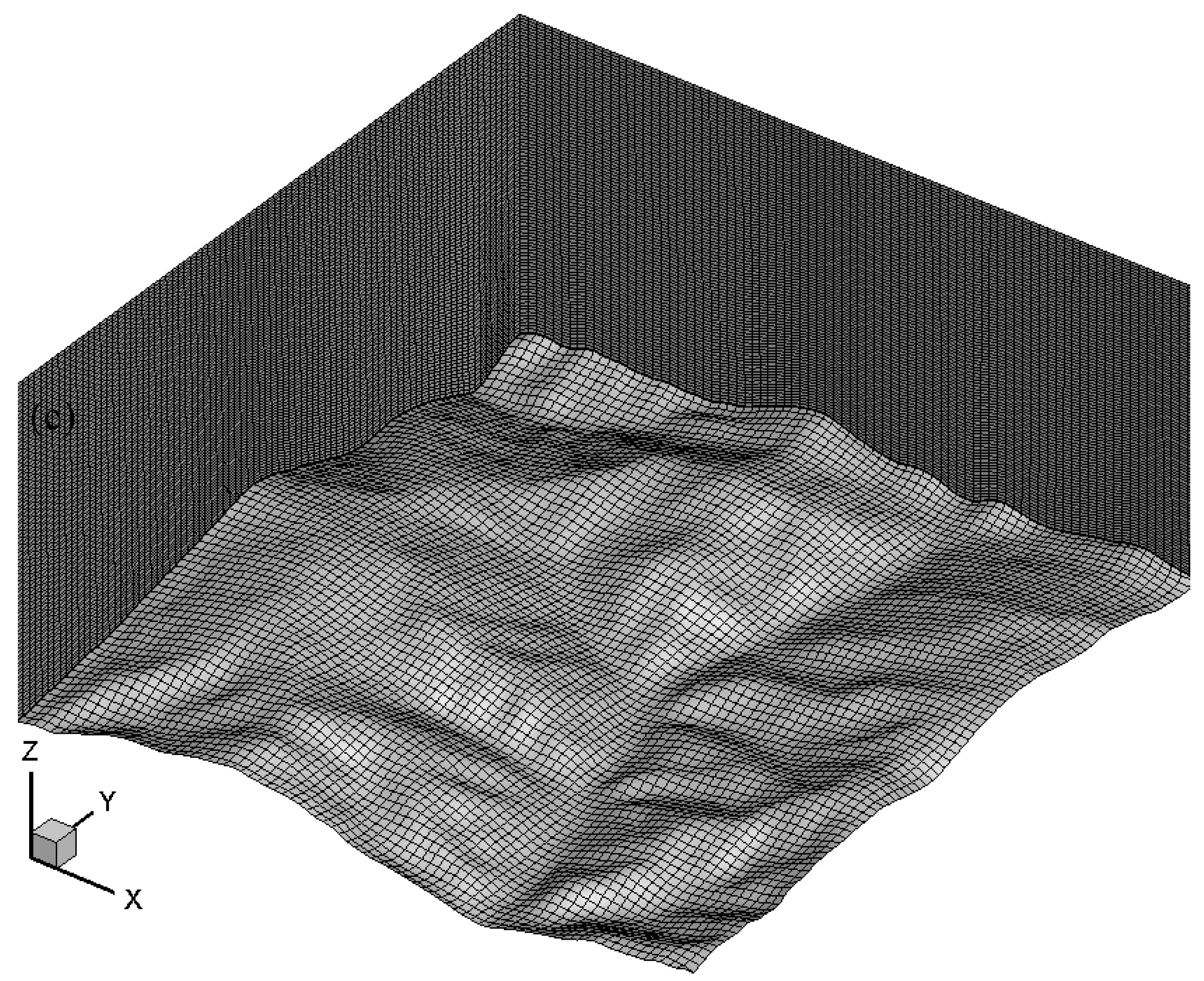
The abrupt terrain of the Chongli Mountain region could greatly affect the atmospheric flow, so a high-resolution terrain is essential for CFD. To achieve a high-quality 3D terrain model, the high-resolution terrain dataset Advanced Spaceborne Thermal Emission and Reflection Radiometer (ASTER) Global Digital Elevation Model (GDEM) [44] was utilized in the CFD domain. A diagram of the CFD configuration based on the ASTER GDEM is shown in Figure 2. Figure 2a shows the topographic distribution of the CFD domain with the three AMSs in the region: AMS-1 is situated on the mountaintop, AMS-2 is on the mountainside, and AMS-3 on the mountain foot. Figure 2b illustrates the 3D terrain model. Figure 2c shows the CFD domain, which is discretized with hexahedral grids [45]. The CFD domain is 4 km × 4 km in the horizontal direction and is 2 km high vertically. The mesh of the CFD domain was established by the GAMBIT software (version 2.4.6), comprising 1.01 × 10⁶ hexahedral cells with a horizontal grid length of 40 m and a vertical grid length of 20 m. Moreover, the height of the first layer in the mesh is 0.1 m from the ground.

2.4. Validation Methodology

To evaluate the accuracy and temporal correlation of numerical simulations, the following indexes were calculated. The indexes below were used for validating both the WRF and WRF-CFD simulations.
Firstly, BIAS means the systematic deviation from expected value. BIAS < 0 reflects underestimation, and BIAS > 0 means overestimation:
BIAS = 1 N i = 1 N ( S i O i ) ,
where O i is the observed wind velocity, S i is the corresponding simulated wind velocity, and N represents the total number of simulated time step.
Secondly, MAE is the mean absolute error from expected values, regardless of underestimation or overestimation:
MAE = 1 N i = 1 N | S i O i | .
Then, MAPE is the mean absolute percentage error from expected values:
MAPE = 1 N i = 1 N | S i O i | O i .
Finally, r is the temporal correlation between observed and simulated wind velocity:
r = i = 1 N ( S i S ¯ ) ( O i O ¯ ) i = 1 N ( S i S ¯ ) 2 i = 1 N ( O i O ¯ ) 2 .
Here, S ¯ represents the mean value of simulated wind velocity and O ¯ reflects the mean value of observed wind velocity.

3. Physical Schemes and Coupling Methods

In this section, an array of 16 WRF simulations based on different physical parameters is described, and two coupling methods used in the WRF-CFD system are compared.

3.1. Physical Schemes

The WRF model offers multiple physical parameterizations that can be combined in any way. Different physical schemes have different impacts on the wind-field simulation for the specific study area or weather phenomenon.
A sensitivity analysis was performed to evaluate which scheme can provide the best boundary conditions for the CFD in the Chongli Mountain region. We tested two different radiation parameters, two land surface parameters, and four PBL parameters to evaluate which scheme is more suitable for the microscale wind-field simulation. Thus, we obtained 16 sets of deterministic simulations.
Table 2 shows the physical schemes used in each WRF simulation. Two sets of shortwave/longwave radiation parameters were tested, one was the Mesoscale Model Version 5 (MM5) [46] with the Rapid Radiative Transfer Model (RRTM) [47], and the other was the new Goddard (NG) [48]. Additionally, two sets of land surface parameters were tested, one was the Noah Land Surface Model (NLSM) [49], and the other was the Rapid Update Cycle (RUC) [50]. A further four sets of PBL schemes were tested, including Yonsei University (YSU) [51], Mellor–Yamada–Janjic (MYJ), Mellor–Yamada–Nakanishi–Niino (MYNN) [52], and the Asymmetric Convective Model version 2 (ACM2). In addition, the microphysics scheme used in the WRF simulation was the WRF single-moment 3-class scheme [53], and the convective parameter used in domains D3 and D4 was the Kain–Fritsch scheme [54].
To choose a suitable physical scheme for the Chongli Mountain region, we tested four different PBL parameterizations, two different radiation parameterizations, and two different land surface parameterizations, totaling 16 sets of deterministic simulations. The period of WRF simulation was from 12:00 on 20 May 2018 to 00:00 on 24 May 2018 (Beijing Time), 84 h in total. The time interval of the model outputs was 1 h, and the first 12 h were considered as a model spin-up. In addition, the observations of AMS-1 were used for numerical simulation validation. To choose the most appropriate physical scheme, the WRF simulations were directly compared with the observed data in terms of the indexes BIAS, MAE, MAPE, and r.

3.2. Coupling Methods

The horizontal and vertical spacings in the CFD model ( Δ x y several tens of meters, Δ z several meters) are very different from those in the WRF model ( Δ x y several kilometers, Δ z several tens of meters). Moreover, the topography of the boundaries in the CFD domain are different from those in the WRF domain. Therefore, coupling the WRF and CFD models is an extremely difficult task.
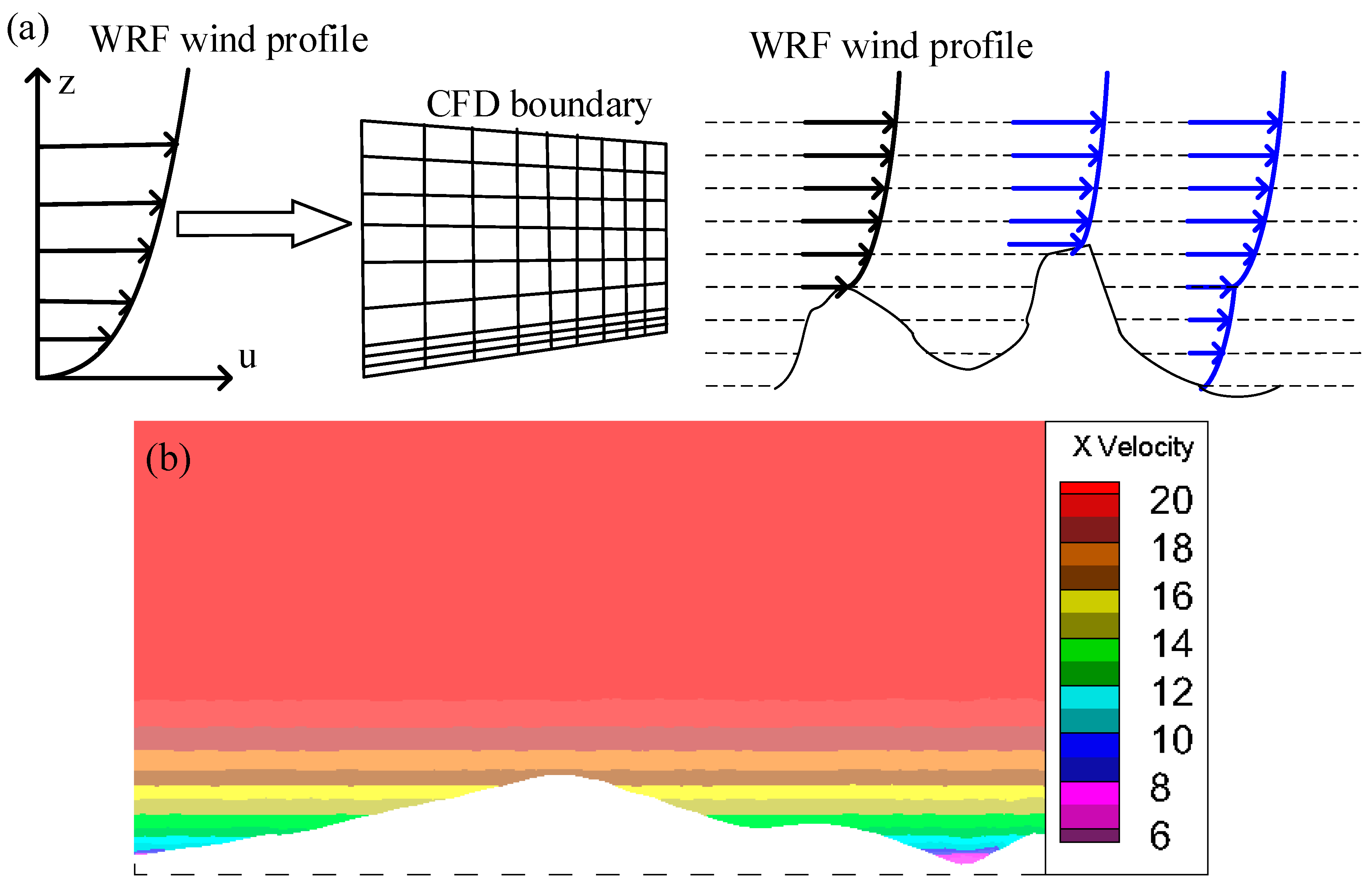
Generally, the coupling method that the WRF-CFD model uses is extrapolation [55]. In extrapolation, a single WRF profile is imposed on an entire inlet face of the CFD domain, and WRF wind data are extrapolated in the CFD grid points that are below or above the WRF profile. Figure 3a depicts a diagram of the extrapolation method over complex terrain. Figure 3b presents the wind velocity on a CFD boundary using extrapolation. From the figure, it can be seen that the distribution of wind velocity on the boundary is uniform in the horizontal direction, which may not correctly describe the effects of actual terrain in the upwind direction. Extrapolation may not be capable of appropriately coupling the WRF and CFD models over complex terrain.
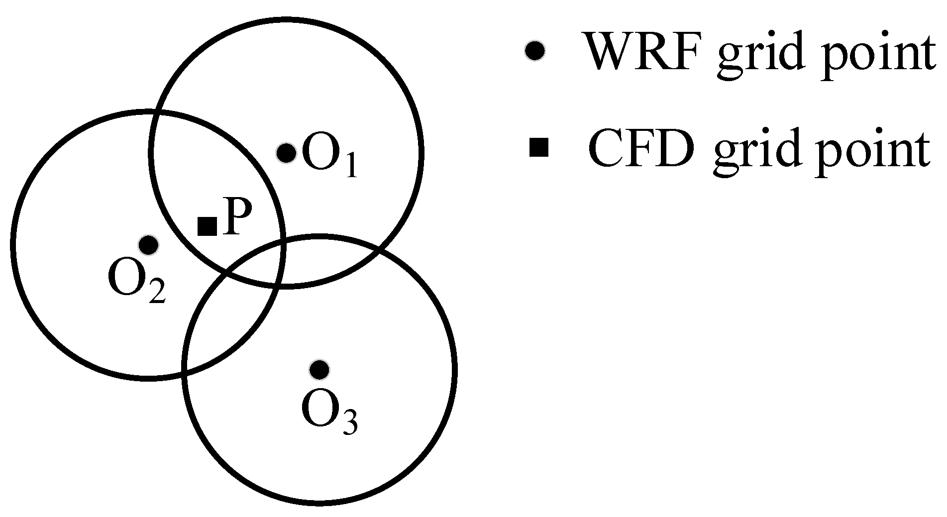
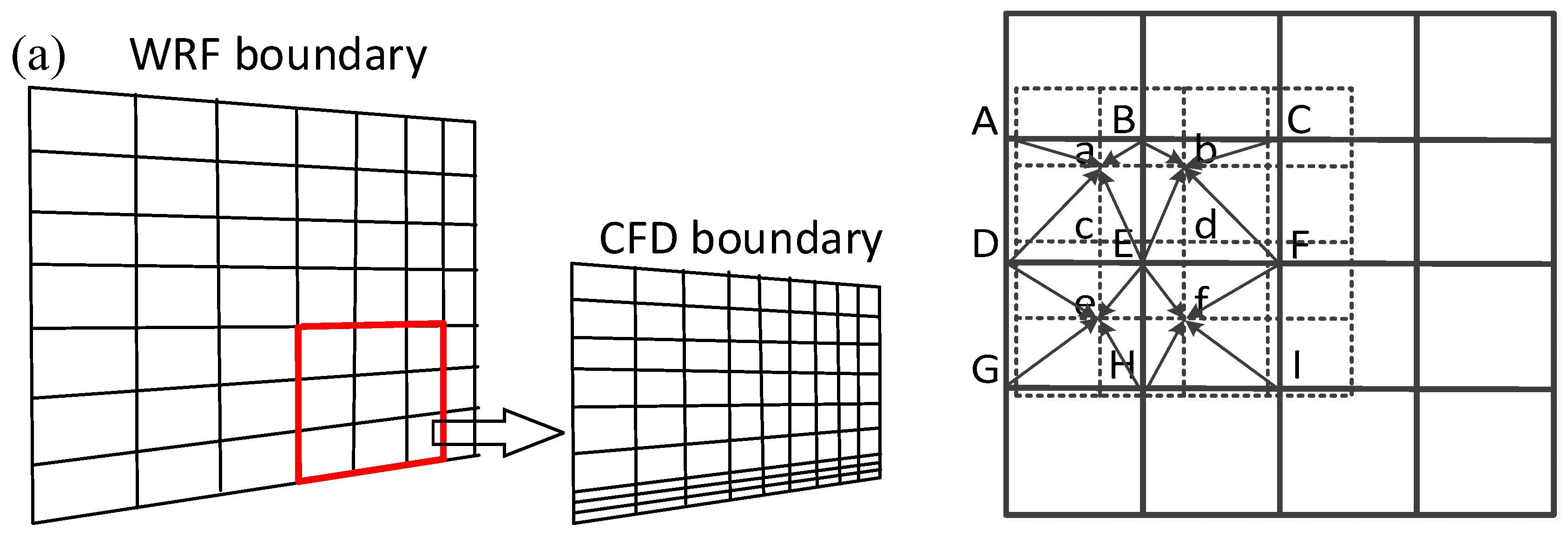
To solve the problem of huge terrain differences between the WRF and CFD models, we used Cressman interpolation [56,57,58] as the coupling method. Figure 4 shows a sketch map of the Cressman interpolation function, where P represents the CFD grid point and O1, O2, and O3 represent the WRF grid points. The black circles indicate the influence range of each WRF grid point. It can be seen that the wind speed at point P is determined by O1 and O2, but not influenced by O3.
When using Cressman interpolation, the wind speed at a CFD grid point only depends on the distances from the nearby WRF grid points:
V i n t e r p o l a t e = i = 1 n W R F V i W i / i = 1 n W R F W i ,
where V i n t e r p o l a t e represents the wind velocity at a CFD grid point; n W R F represents the number of nearby WRF grid points; V i represents the wind velocity at a WRF grid point; and W i represents the weighting function, which depends on the distances between a CFD grid point ( x v a l u e , y v a l u e , and z v a l u e ) and nearby WRF grid points ( x i , y i , and z i ):
W i = w x y · w z = r L 2 d x y 2 r L 2 + d x y 2 · ( 1 | d z | r z ) ,
d x y 2 = ( x v a l u e x i ) 2 + ( y v a l u e y i ) 2 ,
| d z | = | z v a l u e z i | ,
where r L and r z represent the horizontal and vertical influence radii of a WRF grid point, respectively.
Figure 5 illustrates the Cressman interpolation coupling method. Figure 5a shows a diagram of imposing the WRF wind data on the CFD boundary using Cressman interpolation. Figure 5b depicts the wind velocity on a CFD boundary using Cressman interpolation. From the figure, it can be seen that the distribution of the wind velocity on the boundary is more realistic, and the Cressman interpolation may be a more suitable method to couple the WRF and CFD models over complex terrain.

4. Results and Discussion

4.1. Physical Schemes

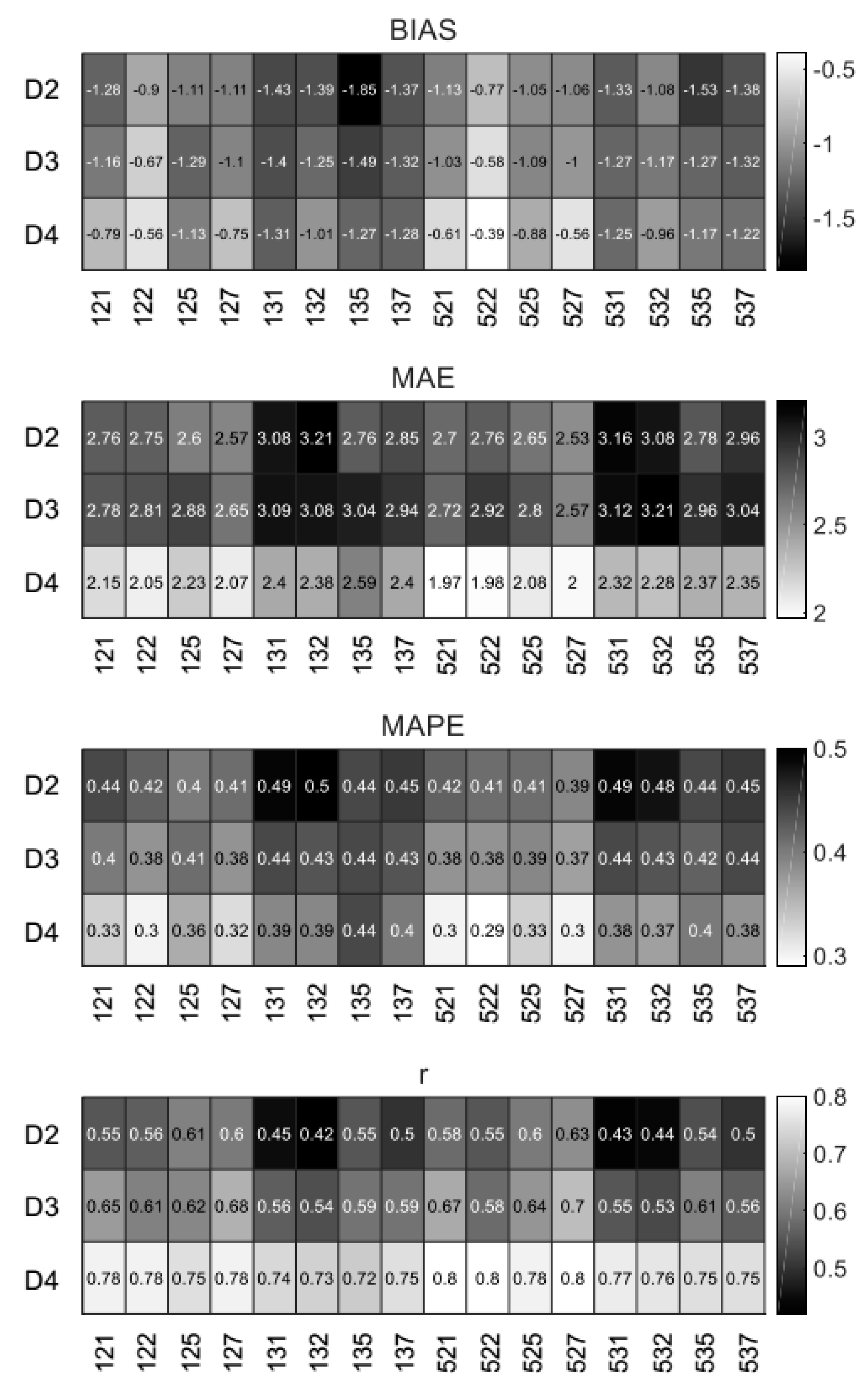
Figure 6 shows the calculated results of the sensitivity analysis for domains D2, D3, and D4 and the 16 simulations. Due to the low horizontal resolution, D1 was not taken into account. The darker gray colors reflect the poorer values (BIAS, MAE, MAPE, and r), while the light gray indicates the better values.
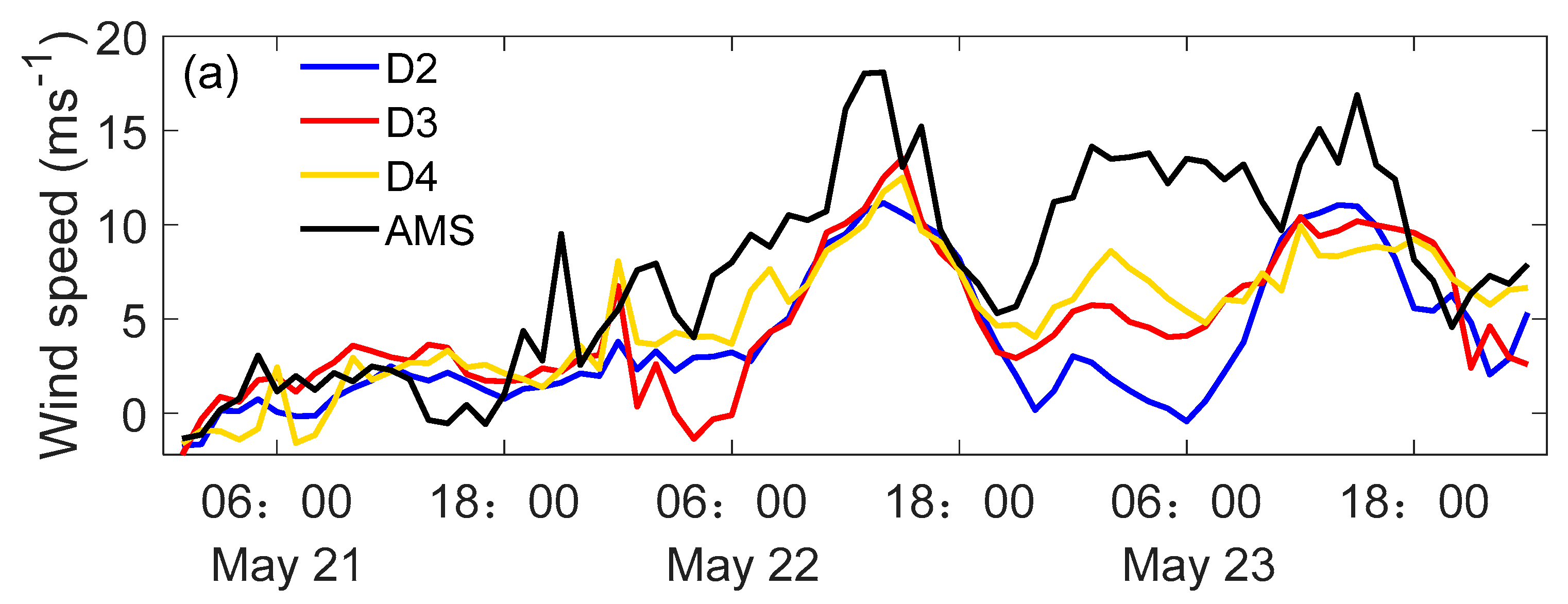
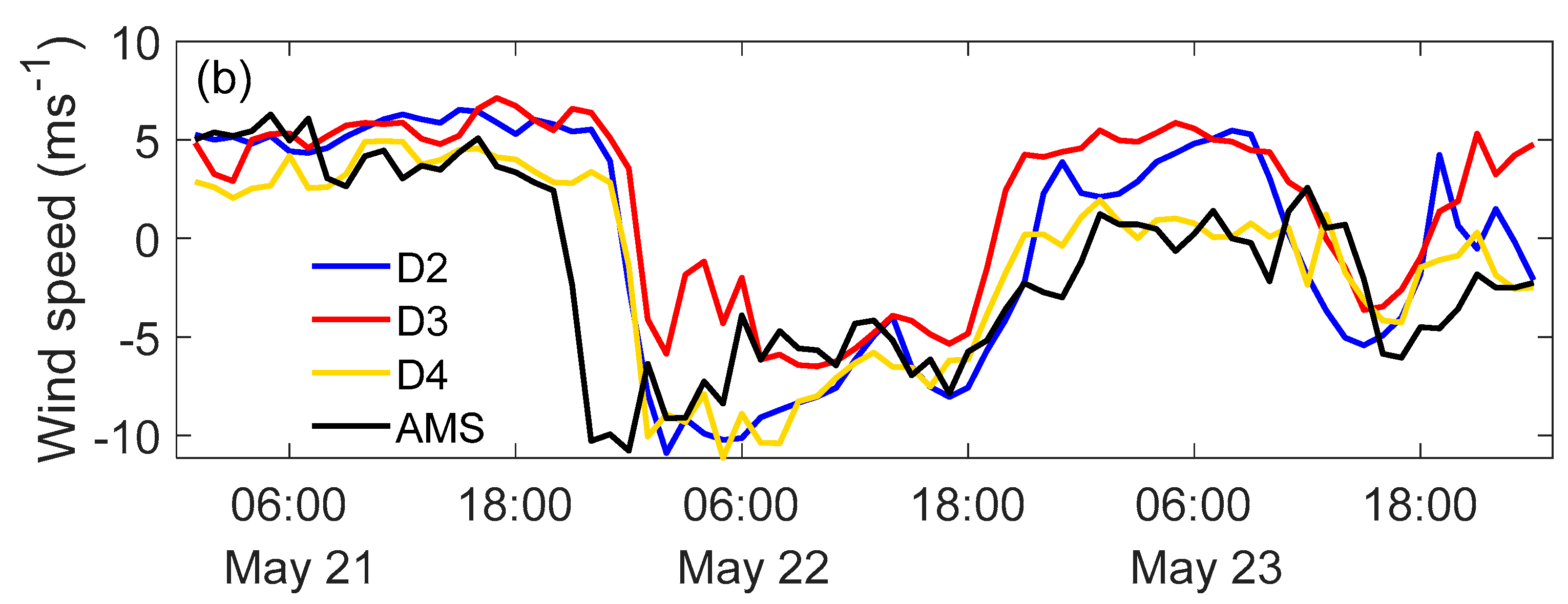
A remarkable improvement of the model accuracy can be seen when the horizontal resolution is increased to 1 km (D4). For example, the BIAS reflects an underestimation (~1.25 ms−1 and ~1.15 ms−1) for D2 and D3, with a slighter underestimation (~0.91 ms−1) for D4. Likewise, MAE, MAPE, and r indicate a sharp improvement in the highest horizontal resolution domain. For example, r increases from ~0.53 and ~0.61 (D2 and D3) to ~0.77 (D4). Figure 7 shows the time series of the simulated wind speeds in different domains. The physical scheme used in the WRF simulation was WRF-125, and the AMS station referenced in this example was AMS-1. From the figure, it can be seen that the wind speed (u and v components) of the WRF simulation for D4 is closer to the observed value than for those of D2 and D3. More specifically, there is a sharp improvement of the model accuracy when the resolution is increased to 1 km (D4).
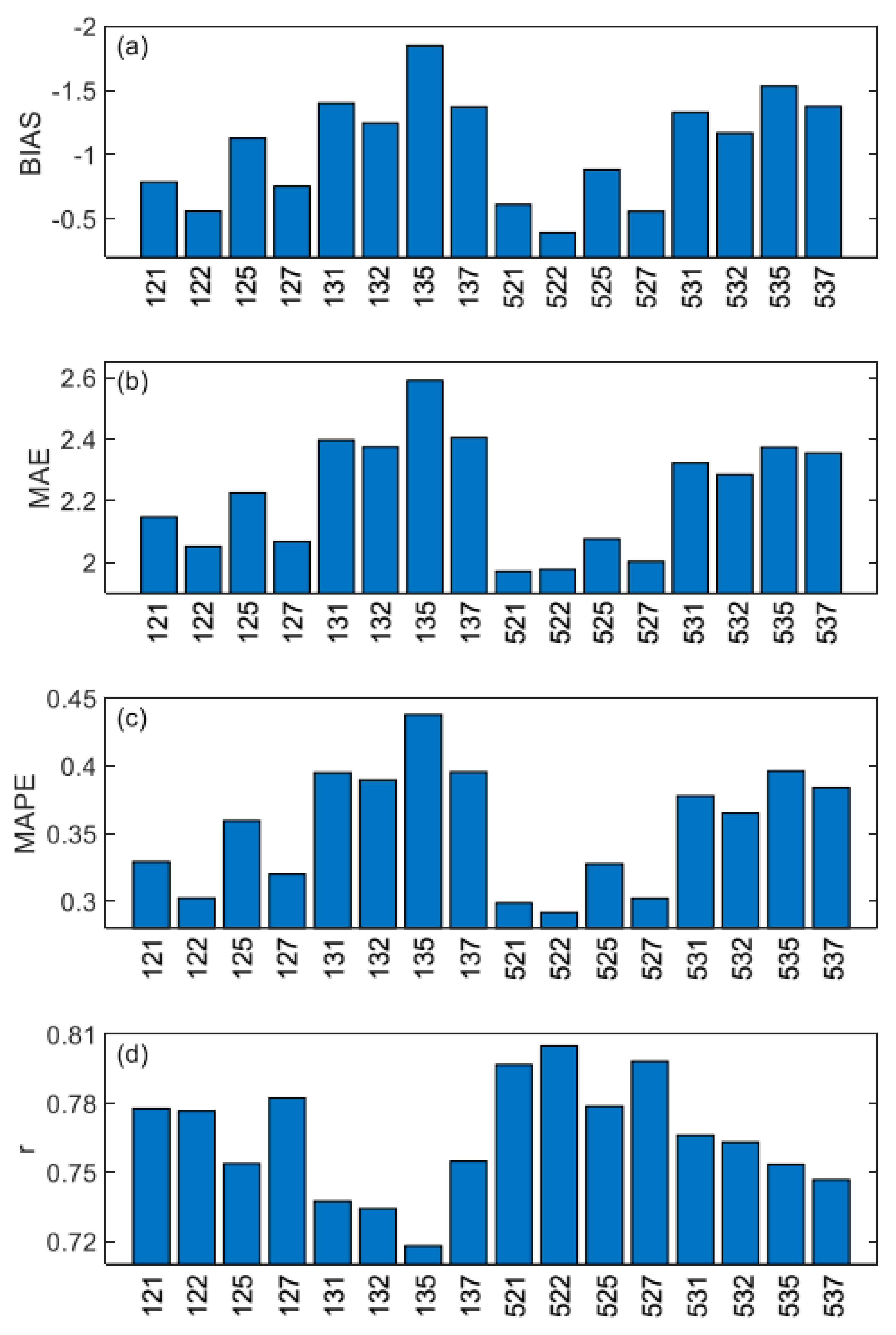
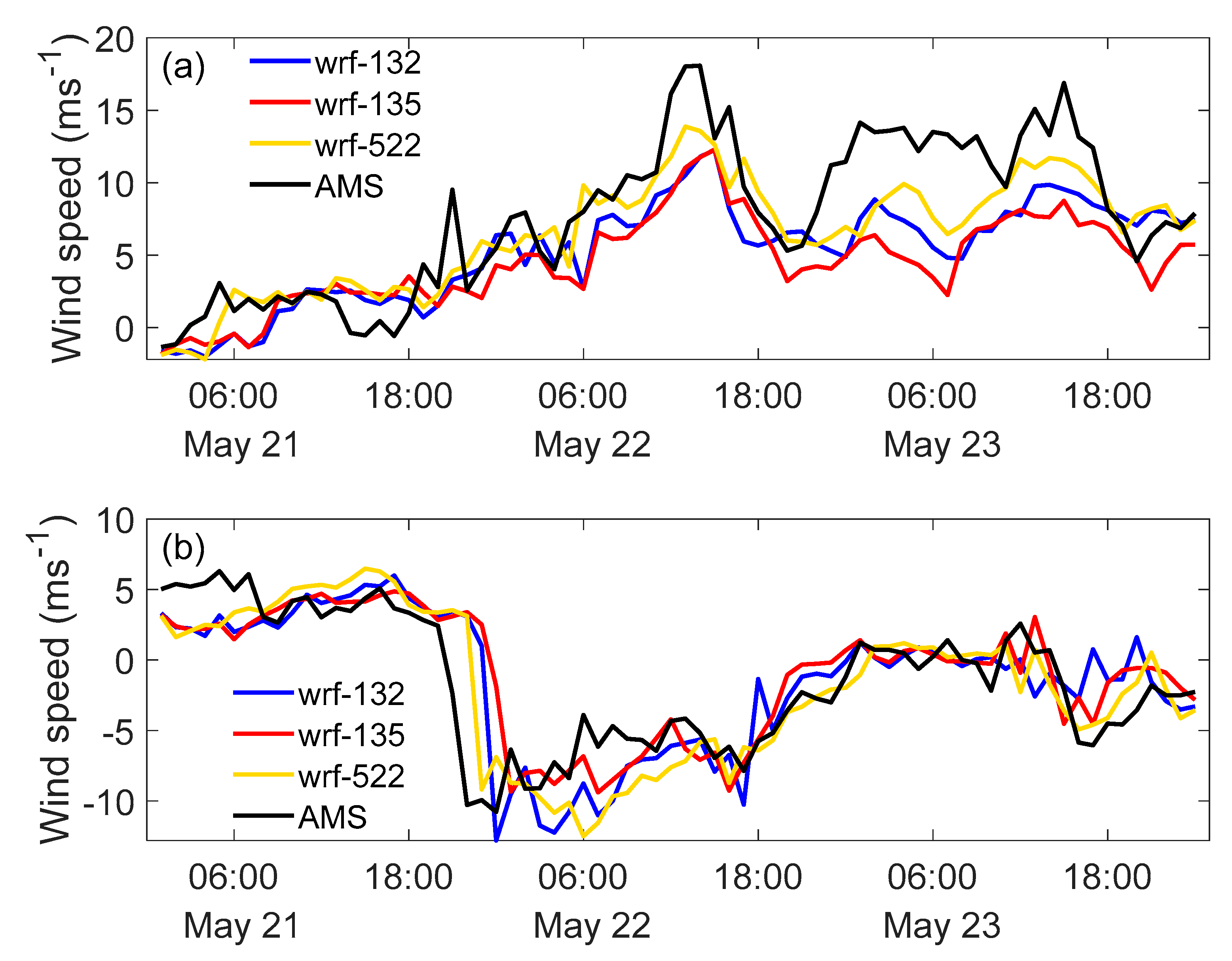
Because the horizontal resolution of 1 km (D4) was the best, the calculated results of the sensitivity analysis are shown in Figure 8 for the domain D4 only. In general, the simulations using the NG/NG radiation scheme were slightly better than those using the MM5/RRTM parameterization. Moreover, the simulations using the NLSM land surface scheme were better than those using the RUC scheme. Meanwhile, the simulations using the MYJ scheme had the best performance, and those using the MYNN scheme had the worst. Prasad et al. [59] explained that the deep mixed layer estimated by MYNN may result in underestimation of the wind speed, contrary to the shallower mixed layer simulated by YSU. Hence, the best performances were achieved with the NG/NG shortwave/longwave radiation scheme, NLSM land surface scheme, and MYJ–PBL scheme (WRF-522) in the Chongli Mountain region. Figure 9 shows the time series of the simulated wind speeds using different physical schemes. Here, the physical schemes used in the WRF simulation are WRF-132, WRF-135, and WRF-522. In addition, the AMS station referenced was AMS-1. From the figure, it can be seen that the wind speed (u and v components) of the WRF simulation initialized with WRF-522 was closer to the observed value than those with WRF-132 and WRF-135.

4.2. Coupling Methods

Two coupling methods were compared in this study: the WRF-CFD model with extrapolation is expressed as WRF-CFD-1, and that with the Cressman interpolation is expressed as WRF-CFD-2. The period of the WRF-CFD simulation was from 00:00 on 21 May 2018 to 00:00 on 24 May 2018 (Beijing Time), 72 h in total. The time interval of the model outputs was 1 h.
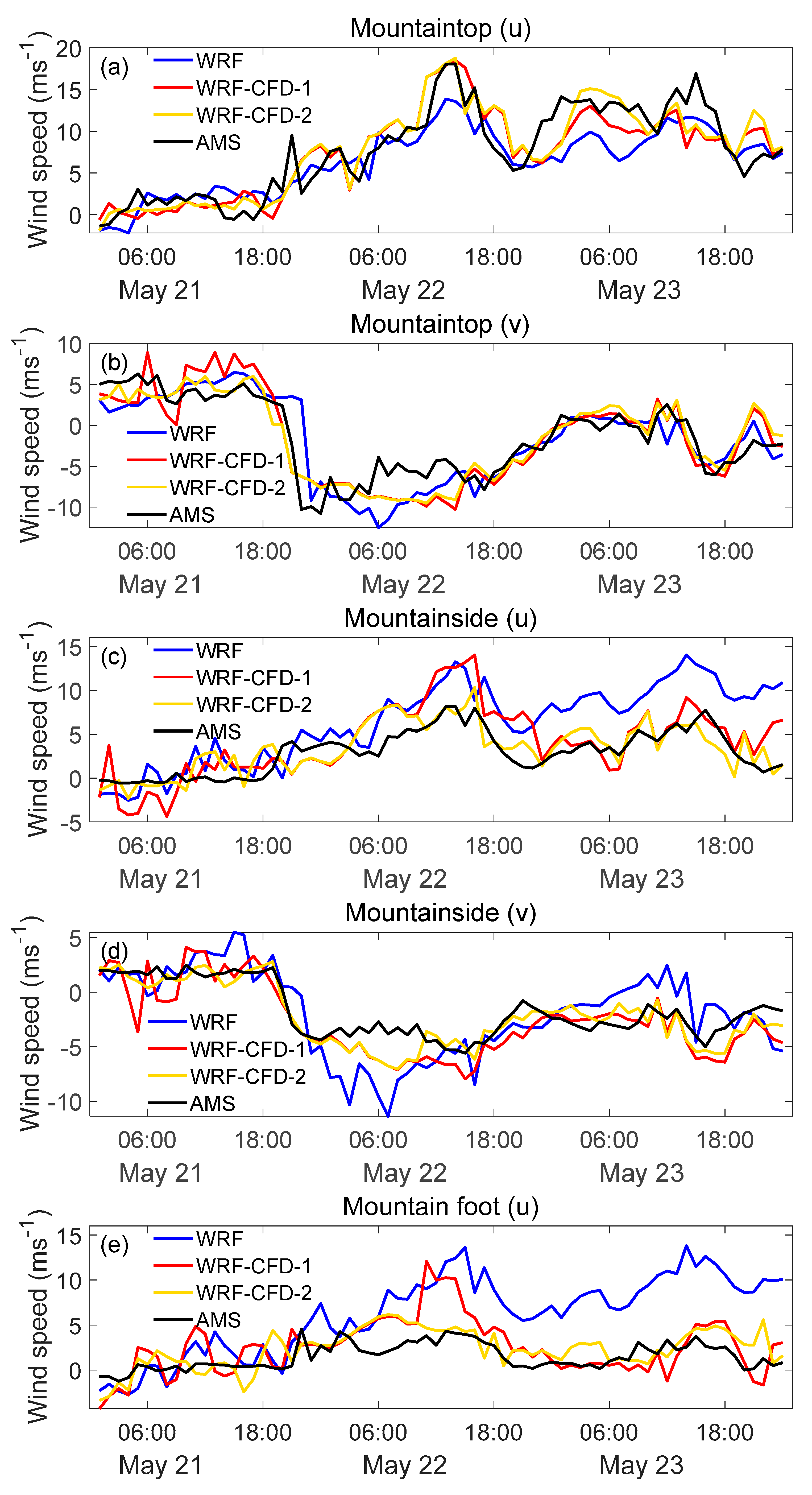
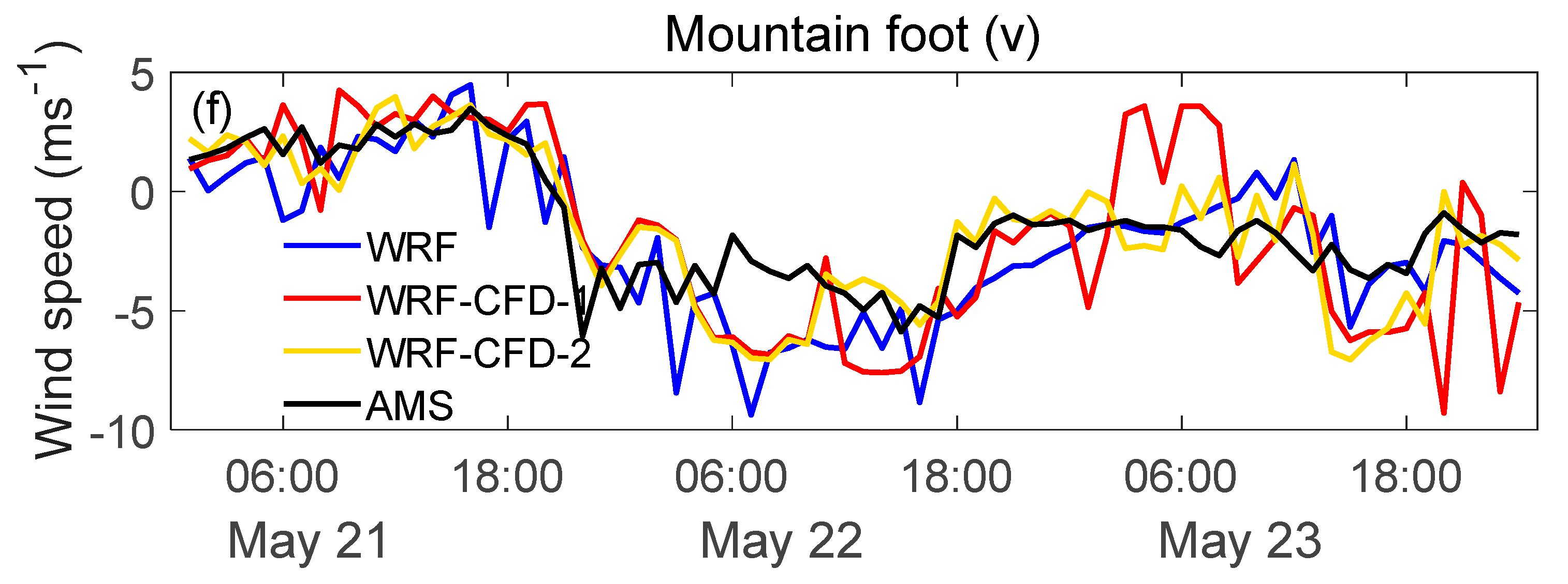
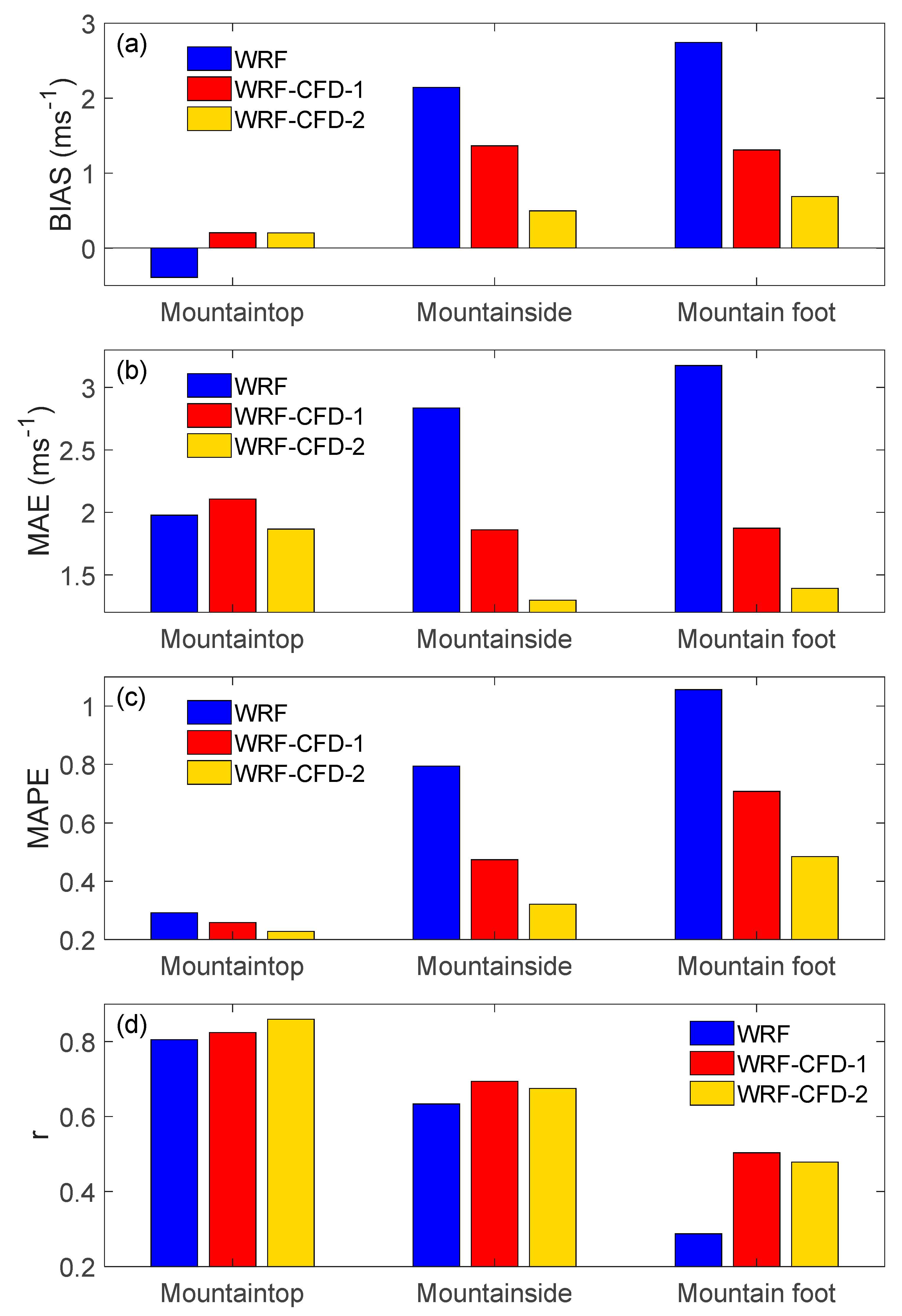
Figure 10 shows the time series of the predicted wind speed using different models: WRF, WRF-CFD-1, and WRF-CFD-2. Figure 11 shows the index BIAS, MAE, MAPE, and r calculated for the simulations of these models. The observation data of the AMS were utilized for numerical model validation. Two conclusions can be drawn from these plots, as follows.
Firstly, WRF-CFD has a better performance than WRF in predicting microscale wind field. For instance, MAE on the mountainside decreased from ~2.84 ms−1 for the WRF simulation to ~1.86 ms−1 for the WRF-CFD-1 simulation, and ~1.28 ms−1 for the WRF-CFD-2 simulation. Likewise, BIAS, MAPE, and r also indicated great improvement from the WRF to the WRF-CFD simulations.
Secondly, the performance of WRF-CFD model using Cressman interpolation (WRF-CFD-2) was better than that using extrapolation (WRF-CFD-1). For instance, BIAS at the mountain foot reflected an overestimation for the WRF-CFD-1 simulation (~1.31 ms−1), and a slight overestimation for the WRF-CFD-2 simulation (~0.68 ms−1). Meanwhile, MAE on the mountainside decreased from ~1.860 ms−1 for the WRF-CFD-1 simulation to ~1.29 ms−1 for the WRF-CFD-2 simulation.
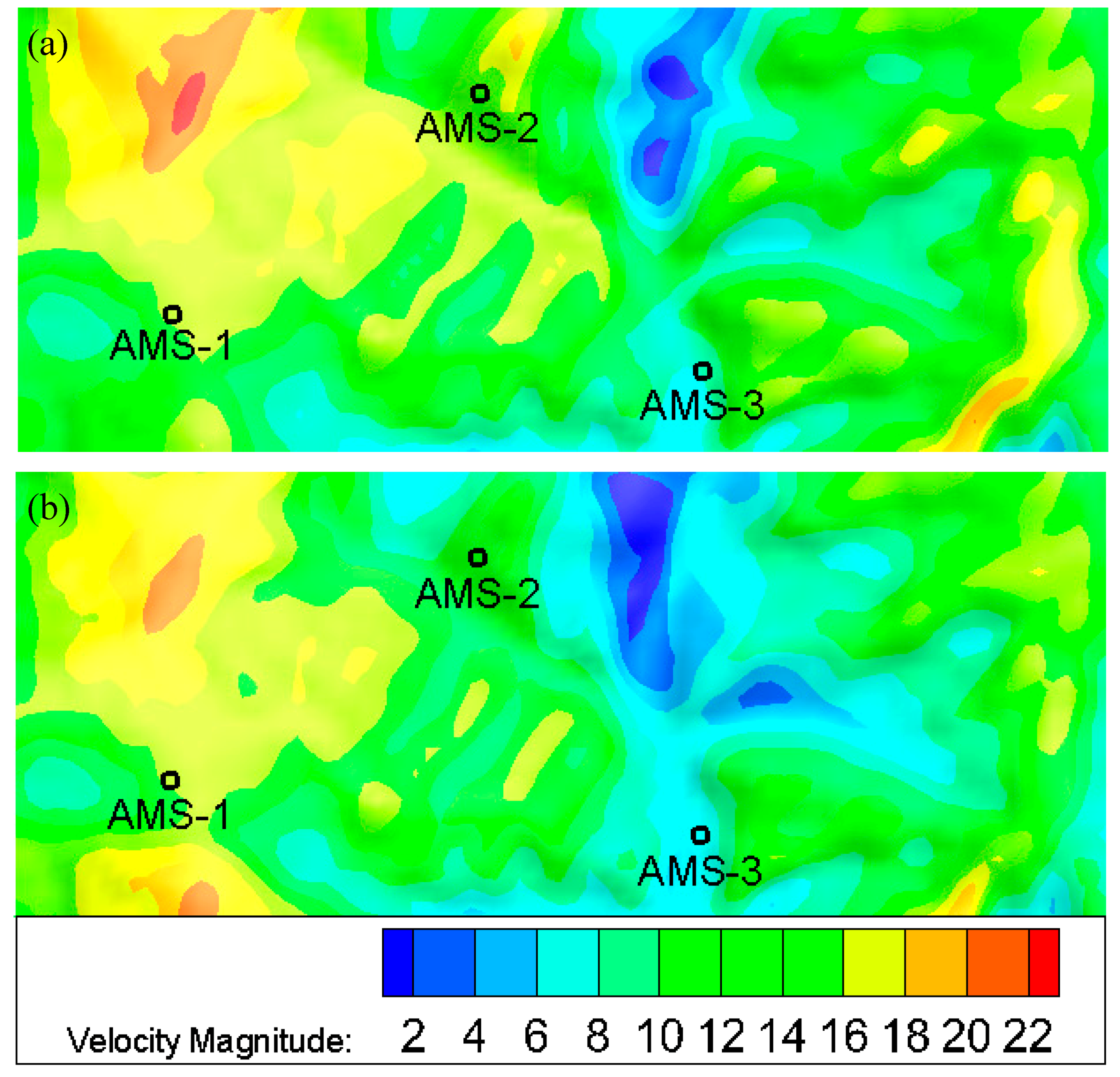
To visually compare the two coupling methods, the local distributions of the near-surface (10 m above ground level (AGL)) wind speed obtained from the WRF-CFD-1 and WRF-CFD-2 simulations are shown in Figure 12. From the figure, it can be seen that the wind fields from the WRF-CFD-1 and WRF-CFD-2 simulations had some differences, while the WRF-CFD-2 simulation had a better performance. For example, the wind speed on the mountainside simulated by WRF-CFD-2 (~11.5 ms−1) was relatively closer to the observed value (~9.2 ms−1) than that by WRF-CFD-1 (~14.2 ms−1). Likewise, the wind speed at the mountain foot simulated by WRF-CFD-2 (~7.1 ms−1) was relatively closer to the observed value (~6.1 ms−1) than that by WRF-CFD-1 (~9.1 ms−1). More specifically, the Cressman interpolation coupling method was more suitable for the microscale wind-field simulation over complex terrain than was extrapolation.

4.3. Microscale Wind Field Simulation

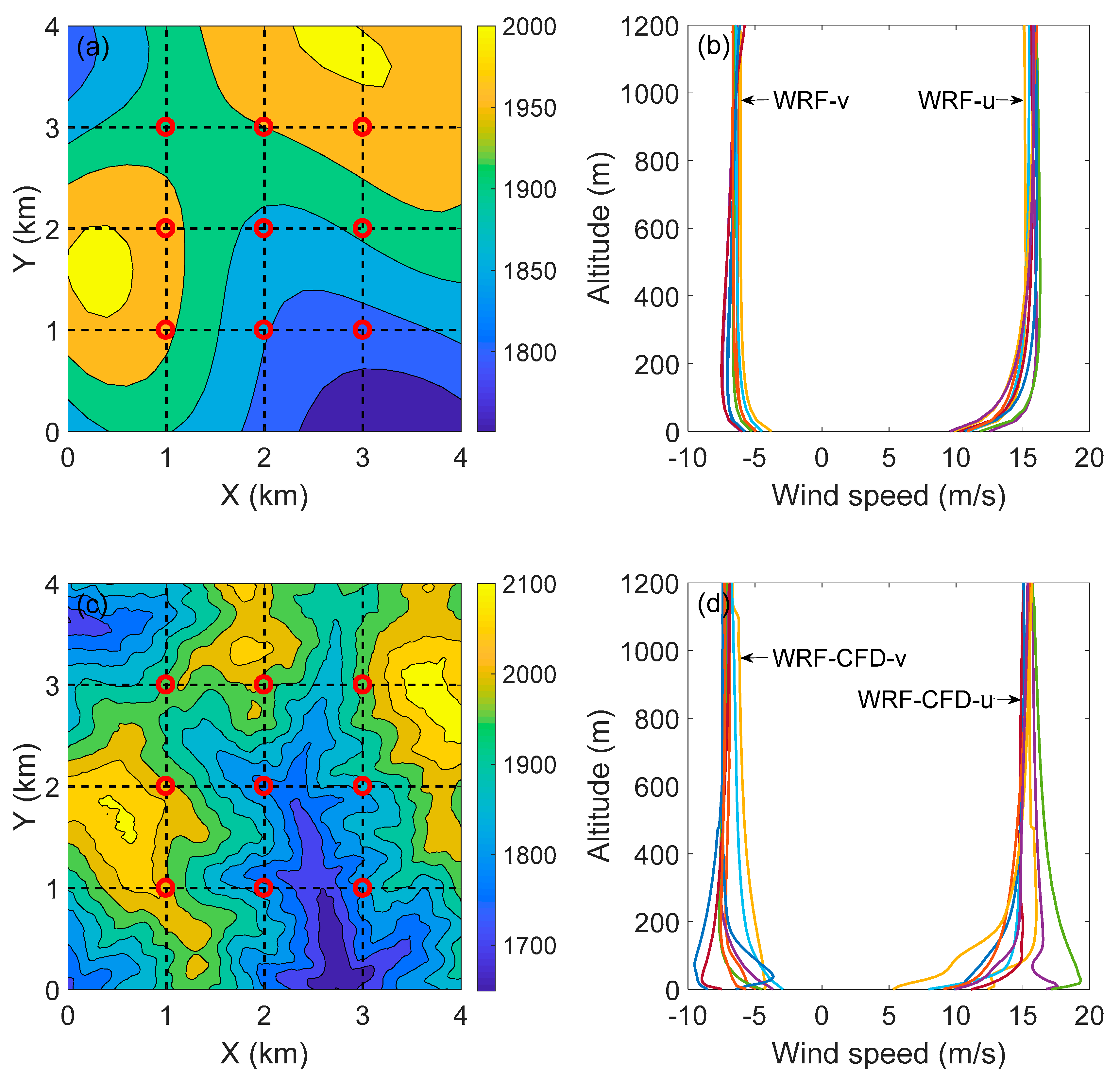
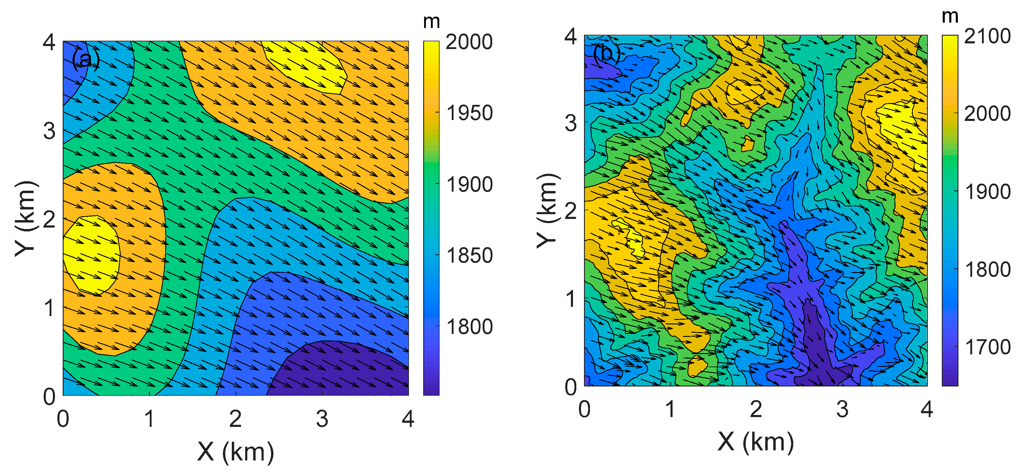
The wind fields from the WRF-CFD simulations were compared with those from the WRF simulations, as shown in Figure 13, Figure 14 and Figure 15.
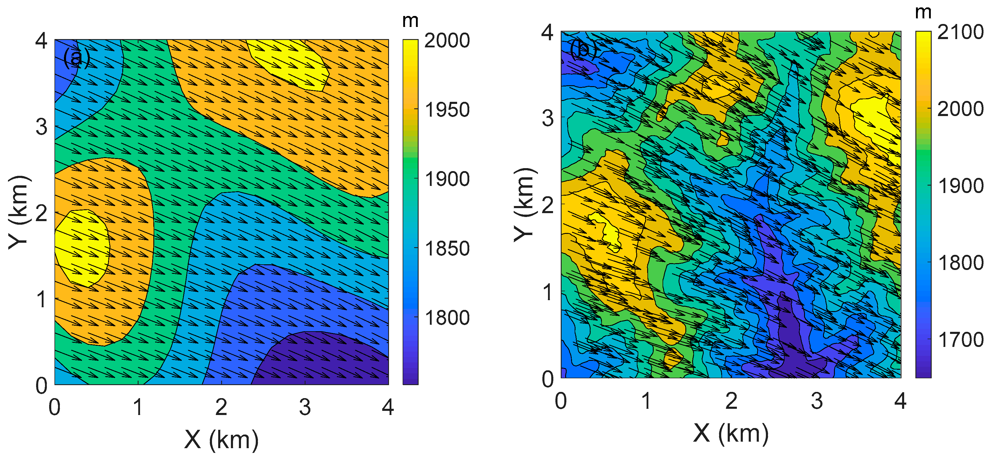
Figure 13 shows the topography and wind profiles simulated by the WRF and WRF-CFD models. The terrain resolution in the WRF model (Figure 13a) was low, and there were small differences among the wind profiles from the WRF simulations (Figure 13b). Thus, WRF cannot simulate the wind field over complex terrain at fine scales. Meanwhile, the terrain resolution in the WRF-CFD model (Figure 13c) was high, and there were significant differences among the wind profiles from the WRF-CFD simulations (Figure 13d) due to the influence of complex terrain.
Figure 14 shows the near-ground wind vectors from the WRF and WRF-CFD simulations. The near-ground wind field simulated by the WRF and WRF-CFD models were generally similar, as the wind directions were northwest in both simulations. However, the details of the wind fields from these two models were quite different. The distribution of the wind field simulated by the WRF model (Figure 14a) was relatively uniform. In contrast, the wind field from the WRF-CFD simulation (Figure 14b) showed more heterogeneity. This difference between the WRF and WRF-CFD simulations may have resulted from the terrain differences between the WRF and CFD models.
Figure 15 shows the wind vectors at 800 m from the WRF and WRF-CFD simulations. The wind fields simulated by the WRF and WRF-CFD models were similar, which may be because the effects of topography on wind are relatively small at high altitudes.

5. Conclusions

A comprehensive understanding of the characteristics of the wind field in the Chongli Mountain region is essential to ensure a successful hosting of the 2022 Olympic Winter Games. In this study, the WRF and CFD models were combined as a one-way off-line nested model system and were applied in a microscale wind simulation in the Chongli Mountain region. The advantage of this system is that the mesoscale model can provide more realistic boundary conditions while the CFD can provide the wind-field simulation with a much higher spatial resolution. The performance of the WRF-CFD model in the Chongli Mountain region will be enhanced by choosing the best physical scheme for WRF and developing an improved coupling method between the WRF and CFD models.
As the WRF model offers multiple physical parameterizations that can be combined in any way, a sensitivity analysis was performed to evaluate which scheme provides the best boundary conditions for the CFD. The results show that the WRF simulation initialized with the NG/NG shortwave/longwave radiation scheme, NLSM land surface scheme, and MYJ–PBL scheme (WRF-522) provides the most suitable boundary conditions for the CFD in the Chongli Mountain region. To overcome the problem of the terrain differences between the WRF and CFD domains, the Cressman interpolation method that couples these two models was proposed. Compared with the extrapolation method, the Cressman interpolation coupling method was more suitable for the coupling of the WRF and CFD models over complex terrain. For example, MAE on the mountainside decreased from ~1.86 ms−1 for the WRF-CFD-1 simulation to ~1.29 ms−1 for the WRF-CFD-2 simulation, and BIAS at the mountain foot decreased from nearly ~1.31 ms−1 to ~0.68 ms−1.
These results can improve the performance of the WRF-CFD model, and signify a more accurate microscale wind simulation in the Chongli Mountain region. However, further work is required, including testing the physical schemes in different seasons and weathers when more observational data are available, as well as testing the coupling methods in other mountainous regions for comparison.

Author Contributions

Writing—original draft preparation, S.L.; supervision, X.S.; data curation, S.Z. (Shan Zhang); investigation, S.Z. (Shijun Zhao); formal analysis, R.Z.

Funding

This research was funded by the National Natural Science Foundation of China, grant number 41575020.

Conflicts of Interest

The authors declare no conflict of interest. The funders had no role in the design of the study; in the collection, analyses, or interpretation of data; in the writing of the manuscript, or in the decision to publish the results.

References

  1. Yamada, T. A numerical-simulation of air-flows and SO-2 concentration distributions in an arid southwestern valley. Atmos. Environ. Gen. Top. 1992, 26, 1771–1781. [Google Scholar] [CrossRef]
  2. Enger, L.; Koracin, D. Simulations of dispersion in complex terrain using a higher-order closure model. Atmos. Environ. 1995, 29, 2449–2465. [Google Scholar] [CrossRef]
  3. Venkatesan, R.; Möllmann-Coers, M.; Natarajan, A. Modeling wind field and pollution transport over a complex terrain using an emergency dose information code SPEEDI. J. Appl. Meteorol. 1997, 36, 1138–1159. [Google Scholar] [CrossRef]
  4. Tong, H.; Walton, A.; Sang, J. Numerical simulation of the urban boundary layer over the complex terrain of Hong Kong. Atmos. Environ. 2005, 39, 3549–3563. [Google Scholar] [CrossRef]
  5. Castelli, S.T.; Reisin, T.G. Application of a modified version of RAMS model to simulate the flow and turbulence in the presence of buildings: The MUST COST732 exercise. Int. J. Environ. Pollut. 2011, 44, 394–402. [Google Scholar] [CrossRef]
  6. Jiménez, P.A.; Gonzálezrouco, J.F.; Garcíabustamante, E. Surface Wind Regionalization over Complex Terrain: Evaluation and Analysis of a High-Resolution WRF Simulation. J. Appl. Meteorol. Clim. 2010, 49, 268–287. [Google Scholar] [CrossRef]
  7. Puliafito, S.E.; Allende, D.G.; Mulena, C.G. Evaluation of the WRF model configuration for Zonda wind events in a complex terrain. Atmos. Res. 2015, 166, 24–32. [Google Scholar] [CrossRef]
  8. Fernándezgonzález, S.; Martín, M.L.; Garcíaortega, E. Sensitivity Analysis of the WRF Model: Wind-Resource Assessment for Complex Terrain. J. Appl. Meteorol. Clim. 2018, 57. [Google Scholar] [CrossRef]
  9. Dudhia, J.; Gill, D.; Manning, K.; Wang, W.; Bruyere, C.; Kelly, S.; Lackey, K. PSU/NCAR Mesoscale Modeling System Tutorial Class Notes and User’s Guide: MM5 Modeling System Version 3; Mesoscale and Microscale Meteorology Division, National Center for Atmospheric Research: Boulder, CO, USA, 2005. [Google Scholar]
  10. Walko, R.L.; Tremback, C.J. RAMS: Regional Atmospheric Modeling System (version 6.0)-Model Input Namelist Parameters; Document Edition 1.4; Atmet LLC: Boulder, CO, USA, 2006. [Google Scholar]
  11. Skamarock, W.C.; Klemp, J.B.; Dudhia, J.; Gill, D.O.; Barker, D.M.; Duda, M.G.; Huang, X.Y.; Wang, W.; Powers, J.G. A Description of the Advanced Research WRF version 3; Mesoscale and Microscale Meteorology Division, National Center for Atmospheric Research: Boulder, CO, USA, 2008. [Google Scholar]
  12. Lundquist, J.K.; Mirocha, J.D.; Chow, F.K.; Kosovic, B.; Lundquist, K.A. Simulating atmosphere flow for wind energy applications with WRF-LES. In Proceedings of the 18th Symposium on Boundary Layers and Turbulence, Stockholm, Sweden, 9 June 2008; American Meteorological Society: Boston, MA, USA, 2008. [Google Scholar]
  13. Li, Y.; Sun, X.; Ning, H.; Qin, H.; Zhao, J. An Analysis of the Physical Characteristics of the Summer Low Atmosphere in the Gobi Desert Adjacent to Bosten Lake, Xinjiang, China. Adv. Meteorl. 2018, 2018, 3061282. [Google Scholar] [CrossRef]
  14. Aitken, M.L.; Kosović, B.; Mirocha, J.D.; Lundquist, J.K. Large eddy simulation of wind turbine wake dynamics in the stable boundary layer using the Weather Research and Forecasting Model. J. Renew. Sustain. Energy 2014, 6, 033137. [Google Scholar] [CrossRef]
  15. Murakami, S.; Mochida, A.; Kato, S. Development of local area wind prediction system for selecting suitable site for windmill. J. Wind Eng. Ind. Aerod. 2003, 91, 1759–1776. [Google Scholar] [CrossRef]
  16. Bitsuamlak, G.T.; Stathopoulos, T.; Bédard, C. Numerical evaluation of wind flow over complex terrain: Review. J. Aerosp. Eng. 2004, 17, 135–145. [Google Scholar] [CrossRef]
  17. Chen, Q. Using computational tools to factor wind into architectural environment design. Energy Build. 2004, 36, 1197–1209. [Google Scholar] [CrossRef]
  18. Blocken, B.; Carmeliet, J.; Stathopoulos, T. Cfd evaluation of wind speed conditions in passages between parallel buildings—Effect of wall-function roughness modifications for the atmospheric boundary layer flow. J. Wind Eng. Ind. Aerod. 2007, 95, 941–962. [Google Scholar] [CrossRef]
  19. Tutar, M.; Oğuz, G. Computational Modeling of Wind Flow Around a Group of Buildings. Int. J. Comput. Fluid D 2004, 18, 651–670. [Google Scholar] [CrossRef]
  20. Li, L.; Hu, F.; Jiang, J.; Cheng, X. An application of the rams/fluent system on the multi-scale numerical simulation of the urban surface layer-a preliminary study. Adv. Atmos. Sci. 2007, 24, 271–280. [Google Scholar] [CrossRef]
  21. Zajaczkowski, F.J.; Haupt, S.E.; Schmehl, K.J. A preliminary study of assimilating numerical weather prediction data into computational fluid dynamics models for wind prediction. J. Wind Eng. Ind. Aerod. 2011, 99, 320–329. [Google Scholar] [CrossRef]
  22. Li, L.; Chan, P.W. Numerical simulation study of the effect of buildings and complex terrain on the low-level winds at an airport in typhoon situation. Meteorol. Z 2012, 21, 183–192. [Google Scholar] [CrossRef]
  23. Miao, Y.; Liu, S.; Chen, B. Simulating urban flow and dispersion in beijing by coupling a cfd model with the wrf model. Adv. Atmos. Sci. 2013, 30, 1663–1678. [Google Scholar] [CrossRef]
  24. Mohan, M.; Sati, A.P. Wrf model performance analysis for a suite of simulation design. Atmos. Res. 2016, 169, 280–291. [Google Scholar] [CrossRef]
  25. Bindu, H.H.; Ratnam, M.V.; Yesubabu, V.; Rao, T.N.; Kesarkar, A.; Naidu, C.V. Characteristics of cyclone generated gravity waves observed using assimilated WRF model simulations over Bay of Bengal. Atmos. Res. 2016, 180, 178–188. [Google Scholar] [CrossRef]
  26. Done, J.; Davis, C.A.; Weisman, M. The next generation of NWP: Explicit forecasts of convection using the weather research and forecasting (WRF) model. Atmos. Sci. Lett. 2010, 5, 110–117. [Google Scholar] [CrossRef]
  27. Carvalho, D.; Rocha, A.; Santos, C.S.; Pereira, R. Wind resource modelling in complex terrain using different mesoscale–microscale coupling techniques. Appl. Energy 2013, 108, 493–504. [Google Scholar] [CrossRef]
  28. Bilal, M.; Birkelund, Y.; Homola, M.; Virk, M.S. Wind over complex terrain–Microscale modelling with two types of mesoscale winds at Nygårdsfjell. Renew. Energy. 2016, 99, 647–653. [Google Scholar] [CrossRef]
  29. Fang, Y.Y.; Xu, H.M.; Zhu, R. Study on Numerical Simulation of Wind Energy Resources Based on WRF and CFD Models. Meteorol. Mon. 2012, 38, 1378–1389. (In Chinese) [Google Scholar]
  30. Temel, O.; Bricteux, L.; Beeck, J.V. Coupled wrf-openfoam study of wind flow over complex terrain. J. Wind Eng. Ind. Aerod. 2018, 174, 152–169. [Google Scholar] [CrossRef]
  31. Carvalho, D.; Rocha, A.; Gómez-Gesteira, M.; Santos, C.S. Offshore winds and wind energy production estimates derived from ASCAT, OSCAT, numerical weather prediction models and buoys—A comparative study for the Iberian Peninsula Atlantic coast. Renew. Energy 2017, 102, 433–444. [Google Scholar] [CrossRef]
  32. Grell, G.A.; Peckham, S.E.; Schmitz, R.; McKeen, S.A.; Frost, G.; Skamarock, W.C.; Eder, B. Fully coupled ‘online’ chemistry within the WRF model. Atmos. Environ. 2005, 39, 6957–6975. [Google Scholar] [CrossRef]
  33. Li, Y.; Lu, G.; Wu, Z.; He, H.; Shi, J.; Ma, Y.; Weng, S. Evaluation of Optimized WRF Precipitation Forecast over a Complex Topography Region during Flood Season. Atmosphere 2016, 7, 145. [Google Scholar] [CrossRef]
  34. Pennelly, C.; Reuter, G. Verification of the Weather Research and Forecasting Model when Forecasting Daily Surface Conditions in Southern Alberta. Atmosphere 2017, 55, 31–41. [Google Scholar] [CrossRef]
  35. Luna, T.; Rocha, A.; Carvalho, A.C.; Ferreira, J.A.; Sousa, J. Modelling the extreme precipitation event over Madeira Island on 20 February 2010. Nat. Hazards Earth Syst. Sci. 2011, 11, 2437–2452. [Google Scholar] [CrossRef]
  36. Teixeira, J.C.; Carvalho, A.C.; Carvalho, M.J.; Luna, T.; Rocha, A. Sensitivity of the WRF model to the lower boundary in an extreme precipitation event—Madeira island case study. Nat. Hazards Earth Syst. Sci. 2014, 14, 2009–2025. [Google Scholar] [CrossRef] [Green Version]
  37. Marques, C.A.F.; Rocha, A.; Corte-Real, J. Comparative energetics of era-40, jra-25 and ncep-r2 reanalysis, in the wave number domain. Dyn. Atmos. Ocean. 2010, 50, 375–399. [Google Scholar] [CrossRef]
  38. Carvalho, D.; Rocha, A.; Gómez-Gesteira, M.; Santos, C.S. WRF wind simulation and wind energy production estimates forced by different reanalyses: Comparison with observed data for Portugal. Appl. Energy 2014, 117, 116–126. [Google Scholar] [CrossRef]
  39. Li, L.; Hu, F.; Cheng, X.L.; Han, H.Y. The application of computational fluid dynamics to pedestrian level wind safety problem induced by high-rise buildings. Chin. Phys. 2004, 13, 1070–1075. [Google Scholar] [CrossRef]
  40. Li, L.; Hu, F.; Cheng, X.L.; Jiang, J.H.; Ma, X.G. Numerical simulation of the flow within and over an intersection model with Reynolds-averaged Navier-Stokes method. Chin. Phys. 2006, 15, 149–155. [Google Scholar] [CrossRef]
  41. Li, L.; Zhang, L.J.; Zhang, N.; Hu, F.; Jiang, Y.; Xuan, C.Y.; Jiang, W.M. Study on the micro-scale simulation of wind field over complex terrain by RAMS/FLUENT modeling system. Wind Struct. 2010, 13, 519–528. [Google Scholar] [CrossRef]
  42. Cabezón, D.; Iniesta, A.; Ferrer, E.; Martí, I. Comparing WAsP and Fluent for highly complex terrain wind prediction. In Wind Energy; Springer: Berlin/Heidelberg, Germany, 2007. [Google Scholar]
  43. Wei, Z.; Deng, Y.C.; Zhang, W.; Yang, Z.H. An empirical study of two numerical models for wind resource simulation in complex terrain. Appl. Mech. Mater. 2014, 535, 8–12. [Google Scholar] [CrossRef]
  44. Hirt, C.; Filmer, M.S.; Featherstone, W.E. Comparison and validation of the recent freely available aster-gdem ver1, srtm ver4.1 and geodata dem-9s ver3 digital elevation models over australia. J. Geol. Soc. Aust. 2010, 57, 337–347. [Google Scholar] [CrossRef] [Green Version]
  45. Haga, T.; Kuzuu, K.; Takaki, R.; Shima, E. Assessment of an Unstructured CFD Solver for RANS Simulation on Body-Fitted Cartesian Grids. In Proceedings of the Aerospace Sciences Meeting 2014, National Harbor, MD, USA, 13–17 January 2014. [Google Scholar]
  46. Dudhia, J. Numerical Study of Convection Observed during the Winter Monsoon Experiment Using a Mesoscale Two-Dimensional Model. J. Atmos. Sci. 1989, 46, 3077–3107. [Google Scholar] [CrossRef]
  47. Mlawer, E.J.; Taubman, S.J.; Brown, P.D.; Iacono, M.J.; Clough, S.A. Radiative transfer for inhomogeneous atmospheres: Rrtm, a validated correlated-k model for the longwave. J. Geophys. Res. 1997, 102, 16663–16682. [Google Scholar] [CrossRef] [Green Version]
  48. Chou, M.D.; Suarez, M.J.; Liang, X.Z.; Yan, M.M.H.; Cote, C. A Thermal Infrared Radiation Parameterization for Atmospheric Studies; NASA Technical Report; NASA Goddard Space Flight Center: Greenbelt, MD, USA, 2001; pp. 56–63.
  49. Chen, F.; Duhia, J. Coupling an advanced land surface hydrology model with the penn state ncar mm5 modeling system. part i: Model implementation and sensitivity. Mon. Weather Rev. 2001, 129, 569–585. [Google Scholar] [CrossRef] [Green Version]
  50. Smirnova, T.G.; Brown, J.M.; Benjamin, S.G. Performance of Different Soil Model Configurations in Simulating Ground Surface Temperature and Surface Fluxes. Mon. Weather Rev. 1997, 125, 1870–1884. [Google Scholar] [CrossRef]
  51. Hong, S.Y.; Noh, Y.; Duhia, J. A new vertical diffusion package with an explicit treatment of entrainment processes. Mon. Weather Rev. 2006, 134, 2318–2341. [Google Scholar] [CrossRef] [Green Version]
  52. Nakanishi, M.; Niino, H. An improved mellor–yamada level-3 model: Its numerical stability and application to a regional prediction of advection fog. Bound. Layer Meteorol. 2006, 119, 397–407. [Google Scholar] [CrossRef]
  53. Cossu, F.; Hocke, K. Influence of microphysical schemes on atmospheric water in the weather research and forecasting model. Geosci. Model Dev. 2014, 7, 147–160. [Google Scholar] [CrossRef] [Green Version]
  54. Kain, J.S.; Fritsch, J.M. Convective parameterization for mesoscale models: The kain-fritsch scheme. Meteorol. Monogr. 1993, 24, 165–170. [Google Scholar]
  55. Laporte, L.; Dupont, É.; Carissimo, B.; Musson-Genon, L.; Sécolier, C. Atmospheric CFD simulations coupled to mesoscale analyses for wind resource assessment in complex terrain. In Proceedings of the European Wind Energy Conference, Marseille, France, 16 March 2009. [Google Scholar]
  56. Wikle, C.K. Atmospheric Modeling, Data Assimilation, and Predictability. Technometrics 2002, 47, 521. [Google Scholar] [CrossRef]
  57. Hewitson, B.C.; Crane, R.G. Gridded area-averaged daily precipitation via conditional interpolation. J. Clim. 2005, 18, 41–57. [Google Scholar] [CrossRef] [Green Version]
  58. Liu, Y.; Yu, J.; Shen, Y.; Lv, X. A modified interpolation method for surface total nitrogen in the bohai sea. J. Atmos. Ocean. Technol. 2016, 33, 1509–1517. [Google Scholar] [CrossRef]
  59. Prasad, K.B.R.R.H.; Srinivas, C.V.; Rao, T.N.; Naidu, C.V.; Baskaran, R. Performance of wrf in simulating terrain induced flows and atmospheric boundary layer characteristics over the tropical station gadanki. Atmos. Res. 2016, 185, 101–117. [Google Scholar] [CrossRef]
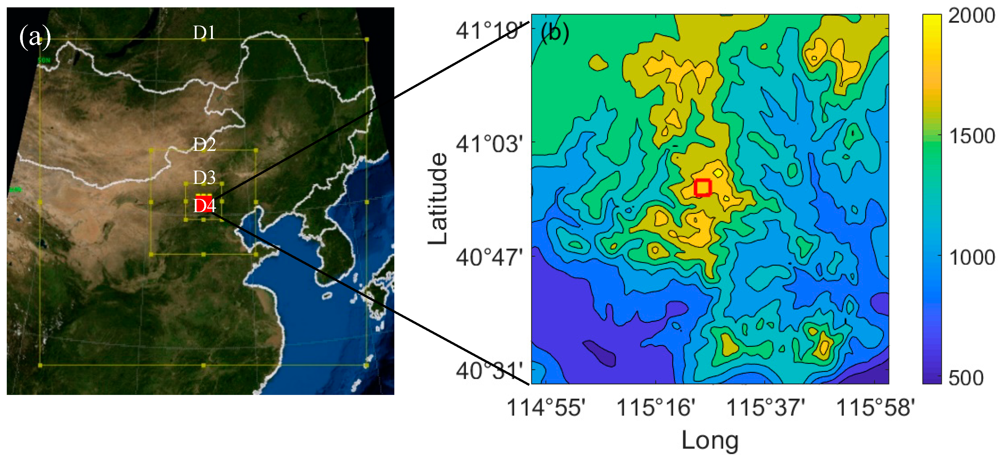
Figure 1. Simulated domain of the Weather Research and Forecasting (WRF) model: (a) Scope of the four nested domains (D1~D4) used in the wind simulation; (b) Topographic distribution of the innermost domain (D4). The red box represents the computational fluid dynamics (CFD) domain, latitude: 40°56′22″–40°58′32″, longitude: 115°23′53″–115°26’45″.
Atmosphere 10 00731 g001
Figure 2. Diagrams of the CFD configuration based on the Advanced Spaceborne Thermal Emission and Reflection Radiometer (ASTER) Global Digital Elevation Model (GDEM): (a) Topographic distribution and the distribution of the automatic meteorological stations (AMSs) (red dots) in the mountain region; (b) 3D terrain model; (c) CFD domain discretized with hexahedral grids.
Atmosphere 10 00731 g002aAtmosphere 10 00731 g002b
Figure 3. Extrapolation coupling method: (a) Diagram of the extrapolation method: A single WRF profile is imposed on an entire CFD boundary, and WRF wind data are extrapolated in the CFD grid points below or above the WRF profile. (b) Wind velocity (m/s) on a CFD boundary using extrapolation, with the horizontal axis (x) showing the width (0–4 km) and the vertical axis (z) showing the height (0–2 km).
Atmosphere 10 00731 g003
Figure 4. Sketch map of Cressman interpolation function. WRF and CFD grid points are all on the lateral boundary of the CFD domain.
Atmosphere 10 00731 g004
Figure 5. Cressman interpolation coupling method: (a) Diagram of imposing the WRF wind data on a CFD boundary using Cressman interpolation. a–f are the CFD grid points, and A–I are the nearby WRF gird points. (b) Wind velocity (m/s) on a CFD boundary using Cressman interpolation, with horizontal axis (x) showing the width (0–4 km) and vertical axis (z) showing the height (0–2 km).
Atmosphere 10 00731 g005aAtmosphere 10 00731 g005b
Figure 6. Panels of BIAS, MAE, MAPE, and r calculated for different domains (D2, D3, and D4) and physical schemes.
Atmosphere 10 00731 g006
Figure 7. Time series of simulated wind speeds for domains D2, D3, and D4: (a) u component (m/s); (b) v component (m/s).
Atmosphere 10 00731 g007aAtmosphere 10 00731 g007b
Figure 8. Histograms of BIAS, MAE, MAPE, and r calculated for domain D4 and 16 simulations: (a) BIAS; (b) MAE; (c) MAPE; (d) r.
Atmosphere 10 00731 g008
Figure 9. Time series of simulated wind speeds using different physical schemes for domain D4: (a) u component; (b) v component.
Atmosphere 10 00731 g009
Figure 10. Time series of predicted wind speed using different models: WRF, WRF-CFD-1, and WRF-CFD-2: (a,b) mountaintop; (c,d) mountainside; (e,f) mountain foot.
Atmosphere 10 00731 g010aAtmosphere 10 00731 g010b
Figure 11. Index BIAS, MAE, MAPE, and r calculated using different models: WRF, WRF-CFD-1, and WRF-CFD-2: (a) BIAS; (b) MAE; (c) MAPE; (d) r.
Atmosphere 10 00731 g011
Figure 12. Local distributions of near-surface (10 m AGL) wind speed (m/s) obtained from the (a) WRF-CFD-1 simulation and (b) WRF-CFD-2 simulation, 16:00 on 22 May 2018.
Atmosphere 10 00731 g012
Figure 13. Topography (m) and wind profiles simulated by the WRF and WRF-CFD models, 16:00 on 22 May 2018: (a,b) WRF simulation; (c,d) WRF-CFD simulation. The red circles indicate the selected wind profile sites.
Atmosphere 10 00731 g013
Figure 14. Topography (m) and near-ground (10 m AGL) wind vectors (m/s), 16:00 on 22 May 2018: (a) WRF simulation; (b) WRF-CFD simulation.
Atmosphere 10 00731 g014
Figure 15. Topography (m) and wind vectors (m/s) at 800 m, 16:00 on 21 May 2018: (a) WRF simulation; (b) WRF-CFD simulation.
Atmosphere 10 00731 g015
Table 1. Parameter settings for nested domains (D1~D4).
DomainHorizontal Resolution (km)Grid PointsTime-Step (s)
D127100 × 100108
D29100 × 10036
D33100 × 10012
D41100 × 1004
Table 2. Physical schemes used in each WRF simulation.
Simulation CodeRadiation Scheme (Shortwave/Longwave)Land Surface SchemePBL Scheme
WRF-121MM5/RRTMNLSMYSU
WRF-122MM5/RRTMNLSMMYJ
WRF-125MM5/RRTMNLSMMYNN
WRF-127MM5/RRTMNLSMACM2
WRF-131MM5/RRTMRUCYSU
WRF-132MM5/RRTMRUCMYJ
WRF-135MM5/RRTMRUCMYNN
WRF-137MM5/RRTMRUCACM2
WRF-521NG/NGNLSMYSU
WRF-522NG/NGNLSMMYJ
WRF-525NG/NGNLSMMYNN
WRF-527NG/NGNLSMACM2
WRF-531NG/NGRUCYSU
WRF-532NG/NGRUCMYJ
WRF-535NG/NGRUCMYNN
WRF-537NG/NGRUCACM2