Article

Statistical Analysis of the Spatiotemporal Distribution of Ozone Induced by Cut-Off Lows in the Upper Troposphere and Lower Stratosphere over Northeast Asia

1
Key Laboratory of Meteorological Disaster, Ministry of Education (KLME)/Joint International Research Laboratory of Climate and Environment Change (ILCEC)/Collaborative Innovation Center on Forecast and Evaluation of Meteorological Disasters (CIC-FEMD), Nanjing University of Information Science & Technology, Nanjing 210044, China
2
The Meteorology Center of Liaoning Province, Shenyang 110166, China
*
Authors to whom correspondence should be addressed.
Atmosphere 2019, 10(11), 696; https://doi.org/10.3390/atmos10110696
Submission received: 26 September 2019 / Revised: 30 October 2019 / Accepted: 7 November 2019 / Published: 11 November 2019
(This article belongs to the Special Issue Atmospheric Turbulence Measurements and Calibration)

Abstract

:
This paper presents the results of a statistical study of the spatiotemporal distribution of ozone in the upper troposphere and lower stratosphere (UTLS) regions induced by cut-off lows (COLs) over Northeast Asia. The analysis was based on high-resolution ERA-Interim ozone data and Atmospheric Infrared Sounder (AIRS) satellite data for the period from 2005–2015. A total of 186 COL events were detected. The observed ozone distribution revealed an ozone-rich region in the upper troposphere (300 hPa) located around the center of the COLs at the time when COLs reached their maximum intensity. This region corresponds to a region of high potential vorticity (PV). In the middle troposphere (500 hPa), enhanced levels of the ozone were distributed in two regions. The maximum concentration was located to the east of the COLs, and a secondary maximum region was in the center of the COLs. Further analysis revealed that this spatial distribution of ozone in the upper troposphere was affected mainly by decreased tropopause. The ozone was subject to a ‘rotary’ transport process in the middle troposphere, influenced mainly by the anticlockwise circulation of the COLs and the surrounding horizontal wind distribution. The temporal variations in ozone anomalies also revealed the ozone distribution patterns and transport processes. The variation in ozone anomalies implied that the magnitude of the ozone increase was closely related to the evolution of COLs lifecycle. The temporal and spatial distributions of the ozone revealed by the statistical analysis of the AIRS satellite data were overall consistent with those of the ERA-Interim data.

1. Introduction

Stratosphere–troposphere exchange (STE), which transports materials through the tropopause, is an important dynamic and chemical process that takes place in the region of the upper troposphere and lower stratosphere (UTLS). STE processes play important roles in controlling the budget of trace substances (e.g., ozone, water vapor, and sulfur dioxide) located in the UTLS region [1]. The processes could potentially affect climate change as well [2,3].
Through studies of STE in the past 20 years, the classical STE circulation model developed by Holton et al. has been updated [4]. Stohl et al. [5] showed that one of the most important achievements is a detailed depiction of the STE process in extratropical areas. The extra-tropical UTLS region (Ex-UTLS) is generally considered to cover a range of 5 km above and below the tropopause [6]. The STACCATO (Stratosphere-Troposphere Exchange in a Changing Climate on Atmospheric Transport and Oxidation Capacity) program [7] and START (Stratosphere-Troposphere Analyses of Regional Transport) –05/08 experiments [8,9] conducted in Europe, and the Tibetan Plateau atmospheric composition project conducted in China [10,11] examined the trace substance distribution in the UTLS region through aircraft-based measurements and other means, which reveals an active stratosphere-troposphere air-mixing process in the Ex-UTLS region. The large quantities of air crossing the tropopause are driven by synoptic and mesoscale processes, such as cut-off lows (COLs) [12], the South Asian High [13], and tropopause folding, as well as exchanges across the isentropic surface caused by nonadiabatic processes such as wave breaking [14,15]. However, the specific mechanisms and details of the involved processes have not been clarified. Therefore, an objective and in-depth understanding of the distribution of tracers and the STE process in the Ex-UTLS region are important.
Cut-off lows occur frequently in the regions of Southern Europe, North America, and Northeastern China–Siberia [16]. The type of COLs detected at 500 hPa in Northeastern China, which is accompanied by a cold core in the middle and upper troposphere, is traditionally called a “northeast cold vortex” [17,18]. This type of COLs is typically displayed as a closed geopotential low with a cold core, which has grown out of a trough and becomes displaced out of the basic westerly current and lies equatorward of this current. Cut-off lows move slowly and usually stay in an area for several days [19]. The COL is an important synoptic scale system associated with extratropical STE in the Northern Hemisphere. Cut-off lows have been studied extensively because they can cause severe weather and contribute to STE [12,20,21]. In the pre-formation stage of a COL, the turbulence near the jet stream likely leads to mixing of the air between the stratosphere and troposphere. During the lifecycle of a COL, due to the interaction of a lower front and an upper front, tropopause folding happens on one flank of the jet stream, which results in the occurrence of STE [22].
Because ozone is present in large quantities in the stratosphere compared to the troposphere, it is frequently used as a tracer for STE events [23,24]. Ozone is a greenhouse gas, and deep STE down to the lower troposphere can also contribute to enhanced ozone levels at the ground surface that affects plant and human health [25,26]. Using ozone sonde, airborne, and air quality measurements data, several studies have shown that stratospheric air invasion was caused by COLs’ contributing to the tropospheric ozone budget over mid-latitudes during the spring and winter time [24,25,27]. In addition, reanalysis data [28] and trajectory models [29] have detected stratosphere-to-troposphere events caused by COLs and tropopause folding. Škerlark et al. [30] used ERA-Interim ozone data to study the global climatology of STE from 1979 to 2011. Their study provided a solid foundation for the investigation of STE using high-resolution ERA-Interim ozone data.
Ozone sounding data in Northeast Asia [31,32], satellite data [33,34], and numerical simulations [35,36] have been used to study STE induced by COLs in Northeast Asia. Song et al. [32] used 89 validated ozone profiles in Changchun, China, to study the influence of COLs on UTLS ozone variations. Their results showed that, on average, COLs induced a 32% increase in the UTLS column ozone (between 4 km below and above the lapse-rate tropopause). Liu et al. [33] studied the effects of a COL process over Northeast China on the total column ozone using Microwave Limb Sounder (MLS) and High Resolution Dynamics Limb Sounder (HIRDLS) satellite ozone data and showed that increases in ozone concentration could be attributed to both the descent of the tropopause and stratospheric ozone invasion into the troposphere. Chen et al. [35] used the Weather Research and Forecasting (WRF) model to simulate the STE process and found evidence of active exchange in a COL pre-formation stage. These case studies have demonstrated that COLs play an important role in the redistribution of ozone in the Ex-UTLS region over Northeast Asia.
Studies of the STE caused by COLs over Northeast Asia have focused mainly on the effect of STE on the concentration of tracers [32], the two-way exchange of tracers [34], the transport trajectory of air [36], and the overall effect of air mass exchange [35,37]. These studies have been limited to individual case studies. Our current understanding of the spatial distribution and temporal evolution of ozone in the UTLS region caused by COLs over Northeast Asia is still very limited. In the present study, using high-resolution reanalysis data and Atmospheric Infrared Sounder (AIRS) satellite data, we examined COL events over Northeast Asia for the period of 2005–2015 and conducted a statistical analysis of the spatial distribution and temporal evolution of ozone in the UTLS region induced by COLs. The aim was to determine the effect of COLs on the ozone redistribution in the UTLS region.
The remainder of the paper is organized as follows. The meteorological and ozone data obtained from ERA-Interim reanalysis and AIRS observations are described in Section 2. Section 2 and the appendix also provide details of the analysis methods. In Section 3, the spatial distributions and temporal evolution of the ozone in the UTLS region revealed by the two data sources are analyzed in detail. In Section 4, we present a summary and discussion.

2. Data and Methodology

2.1. Ozone and Meteorology Data

In our study, ERA-Interim, 6-h reanalysis dataset with 2.5° × 2.5° horizontal resolution and 37 vertical pressure levels of geopotential height, temperature, and the horizontal wind field was used to identify COL events in Northeast Asia for the period of 2005–2015.
ERA-Interim ozone dataset with 0.125° × 0.125° horizontal resolution and 6-h temporal resolution was used in a statistical analysis of the ozone distribution in the UTLS region induced by COLs in the 11-year period from 2005 to 2015. These data, which have high spatiotemporal resolution, were sufficient to capture important synoptic data to meso-scale STE processes. The 0.125° × 0.125° monthly mean ozone data were used for calculating the mean state of the ozone over the 11 years. When analyzing the impact of COLs on the distribution of ozone, 6-h ERA-Interim meteorological re-analysis datasets with 0.125° × 0.125° horizontal resolution, such as geopotential height, potential vorticity, and the horizontal wind field, were also used in our statistical analysis.
As a cross-validation, the same statistical analysis was also applied using satellite observations from Level 2 ozone data from AIRS version 6 products. The AIRS satellite scanning process is divided into ascending and descending orbits. It scans the earth for one lap (one ascending orbit and one descending orbit), which takes about 96 min, and makes a total of 15 laps per day. The horizontal and vertical resolutions of AIRS data at the satellite’s nadir point are 13.5 km and 1 km, respectively, and the error in the ozone data of Level 2 below 0.5 hPa is 10%–50% [38]. Using ozone sonde data in USA and China, Monahan et al. [39] and Bian et al. [31] revealed that AIRS retrieval in the UTLS region shows a statistically significant positive correlation with the ozone sonde data. They indicated that, while the absolute values have a large uncertainty, the retrieval captures the variability of ozone in the UTLS region. Therefore, the AIRS ozone data provide good-quality, high-resolution profiles and enough samples to statistically analyze the ozone distribution in the UTLS induced by COLs.

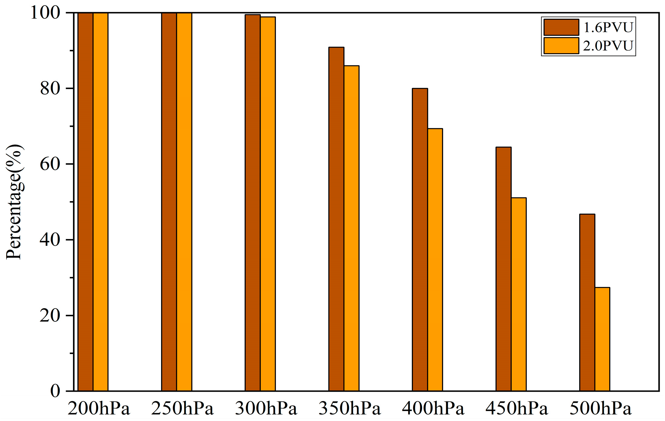
2.2. Methodology for Identifying Cut-Off Lows

A COL is usually identified by analyzing the closed geopotential contours with a cold core on isobaric maps in the middle and upper troposphere [40,41]. Climatological studies of COLs were based on objective or subjective methods, as summarized by Nieto et al. [16].
Nieto et al. [16] used 41 years of National Centers for Environmental Prediction/National Center for Atmospheric Research (NCEP/NCAR) reanalysis data and applied an objective method to investigate the climatology of COLs in the Northern Hemisphere. Their favored formation regions were Southern Europe to the eastern Atlantic coast, the Eastern North Pacific, and the Northern China-Siberia region (the domain extends from 35° N to 65° N and from 100° E to 180° E, which was also used in our study and is referred to as Northeast Asia). The method used by Nieto et al. [16] was mainly based on the geopotential minimum, cutoff circulation, equivalent thickness, and thermal front parameters as the diagnostic conditions. It comprehensively considers the physical characteristics of a COL, and is, therefore, widely used [42,43,44].
Cut-off low events were identified by the objective method of Nieto et al. [16]. We used the 500 hPa geopotential height instead of the 200 hPa proposed by Nieto et al. [16] because COLs in Northeast Asia are typically present in the middle troposphere and have their most distinct characteristics at 500 hPa [17,18]. A grid point was considered a minimum if its geopotential height was lower than the eight surrounding grid points for at least eight time steps (two days). For all cases selected by the previous step, a subjective synoptic analysis was performed at 500 and 300 hPa to ensure a cut-off circulation with a cold core.

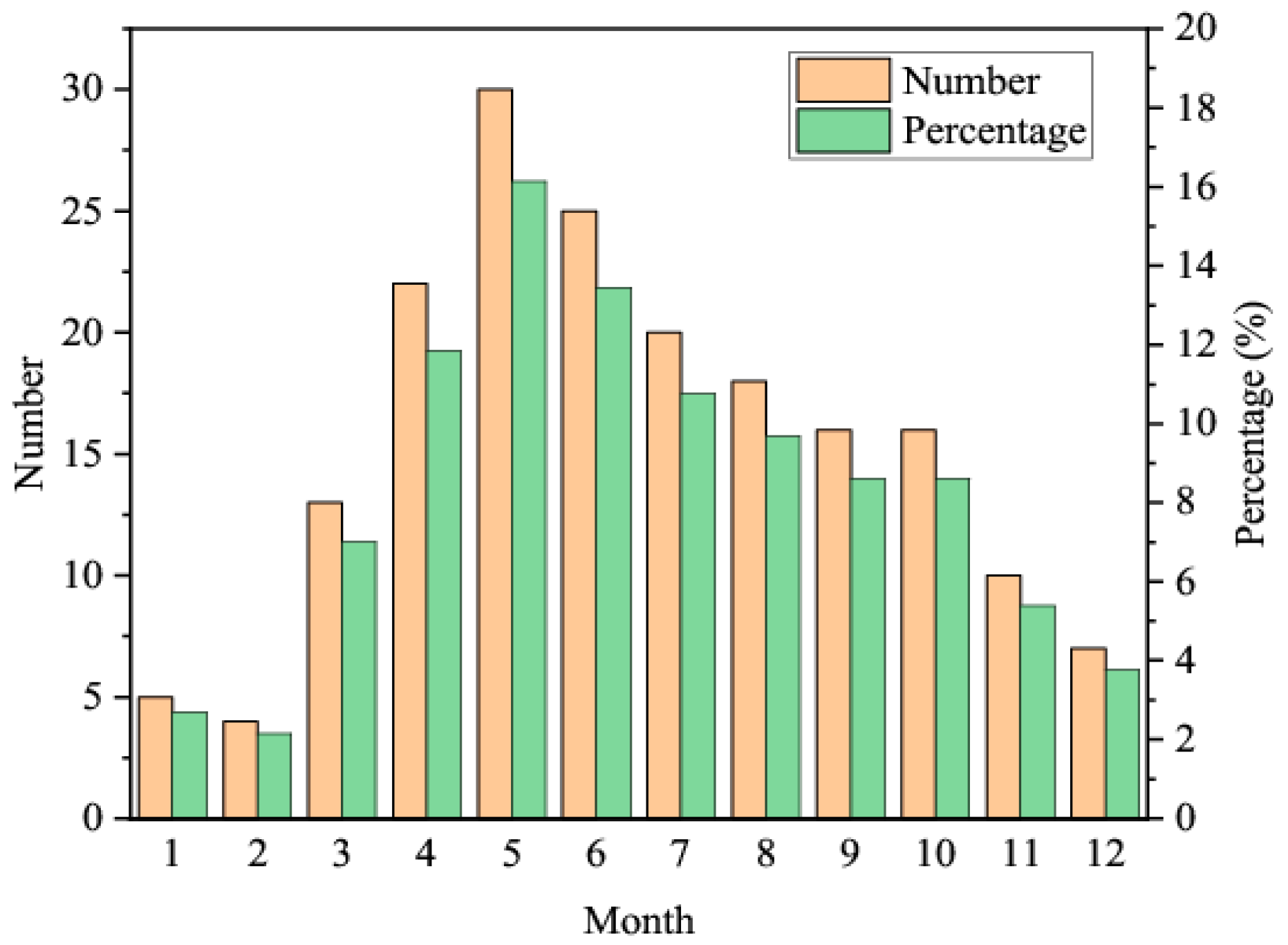
2.3. Statistical Analysis of Cut-Off-Lows in Northeast Asia

Using the 2.5° × 2.5° horizontal resolution data described in Section 2.1 and the method described in Section 2.2, a total of 186 COL events were identified in Northeast Asia in the 11-year period. Figure 1 shows the monthly distribution of COLs during this period, which clearly shows strong seasonal variations. The COLs mainly occurred in the late spring (May), with 16.13% of all cases, followed by early summer (June), with 13.44% of all cases. Spring and summer (from March to August) accounted for 68.82% of all cases during the 11 years. This seasonal pattern was consistent with observations made previously [18].
The magnitude of the potential vorticity (PV) in the stratosphere is higher than that in the troposphere because PV is dependent on temperature. The PV is conservative under adiabatic and frictionless conditions. Thus, it can be used as a dynamic tracer [45]. It has been defined by the World Meteorological Organization (WMO) [46] that a PV value of 1.6 × 10⁻⁶ m2 K kg−1 s−1 (1.6 PV units or PVU) represents the dynamical tropopause and statistical research have displayed that the global dynamical tropopause fall in the range of 1.6 to 3.5 PVU [47].
Figure 2 is presenting the percentage ratio of the COLs in which certain PV (1.6 PVU, 2.0 PVU) isolines dip below different barometric surfaces to the total 186 COL events. It is aimed to preliminarily demonstrate that stratospheric air invasion into UTLS occurs in most of the selected COL cases and provide evidence for the later analysis of the UTLS ozone distribution in Section 3.
It can be observed in Figure 2 that the 2.0 PVU isoline dips below the surface of 250 hPa in all the chosen COL events (100%) while the percentages decrease as the decline of the altitude and the invasion below the barometric surface of 450 hPa in only half (~50%) of the COLs. The climatologic tropopause in the mid-high latitudes is around 9–12 km (namely 300–200 hPa), which has been used to divide the stratosphere and the troposphere. The 2.0 PVU has been used widely as the representative of the stratospheric air regarding the discussion of STE so far, especially in the Northeast Asian region [33,36]. Suppose that the tropopause is at 300 hPa. It is likely to indicate the occurrence of stratospheric air invasion if the 2.0 PVU isoline can dip below the surface of 300 hPa. Figure 2 shows that most COL events (98.9%) were accompanied by the downward transport of stratospheric air to the UTLS region.

2.4. The COLs Coordinates

Using the ERA-Interim reanalysis and AIRS ozone data, we applied the statistical synthesis and matching methods to analyze the ozone distribution and evolution of COLs in the UTLS. Detailed descriptions of these processes are provided in Appendix A and Appendix B, respectively. We give a summary of these methods in this section.

2.4.1. The COLs Coordinate of ERA-Interim Dataset

A total of 186 COL events have been identified in Section 2.2 and the lifecycle of them is divided into four stages: pre-formation, formation, mature, and decay stages based on the ERA-Interim reanalysis. A representative time was identified in each stage to display the whole evolution process of the COLs. Lastly, the synthetic analysis of each COL event in the total 186 COLs was conducted in each stage. Take the time when the COL reaches its strongest intensity as an example. The synthetic analysis was conducted in the following way. The research region was defined by using the point with the lowest geopotential height in each COL at 500 hPa as the central point and extending seven latitudes and longitudes in four directions from it. The research regions of the 186 COLs were coordinated based on the central point of each COL and were converted into a unified COL coordinate. All pressure levels replicated this method.
All the variables analyzed in Section 3.1 and Section 3.2 are based on this coordinate. Take the ozone as an instance. The ozone concentration on each grid point in the research region in each COL case was summed and the average was calculated as the composite mean ozone concentration in the 186 COL events. As for the ozone anomalies, the mean ozone concentration over the whole 11 years is first computed using the ERA-Interim reanalysis, such as the average of the monthly ozone concentration (132 values) on each grid point over the whole time period. Afterward, ozone anomaly values of 186 cases are calculated one by one by subtracting the mean ozone concentration from the ozone concentration in each COL research region. Lastly, the average ozone anomalies in the total COL events are synthetically averaged in the COLs coordinate, which can be regarded as the mean ozone anomalies. It is worth noting that all the variables in Section 3.1 and Section 3.2 refer to the synthetically analyzed variables in the COLs coordinate, which are averaged based on the 186 COL cases in order to demonstrate the overall mean state of the total COLs.

2.4.2. The COLs Coordinate of the AIRS Dataset

Similarly, four stages are divided in Section 3.3 and a representative time is identified in each stage based on the ERA-Interim reanalysis. The footprints in AIRS data are chosen by comparing with the reference points in the ERA-Interim reanalysis, which is selected based on the time and place in which a certain COL event happens.
The time difference between the AIRS data and the ERA-Interim reanalysis is neglected and it is considered an appropriate footprint within the error of 3 h. As for the spatial matching, the research region is set to be a circular region so as to calculate more simply since satellite data consists of irregular orbital data instead of regular grid points in the ERA-Interim. The research region is defined as a circular region with a radius of 7° zonal distance (about 778.4 km) and the center point of the COLs as the center of the circle. If the footprints are within the research region that is based on the calculation of the spherical distance and direction between the footprints and the circle center, they can be regarded as properly chosen. The temporal and spatial matching should both be reached to consider an appropriate footprint as a sample point and the ozone concentration of selected points in the total COL events are marked with dots in the research region.

3. Statistical Analysis of the Ozone Characteristics of COLs

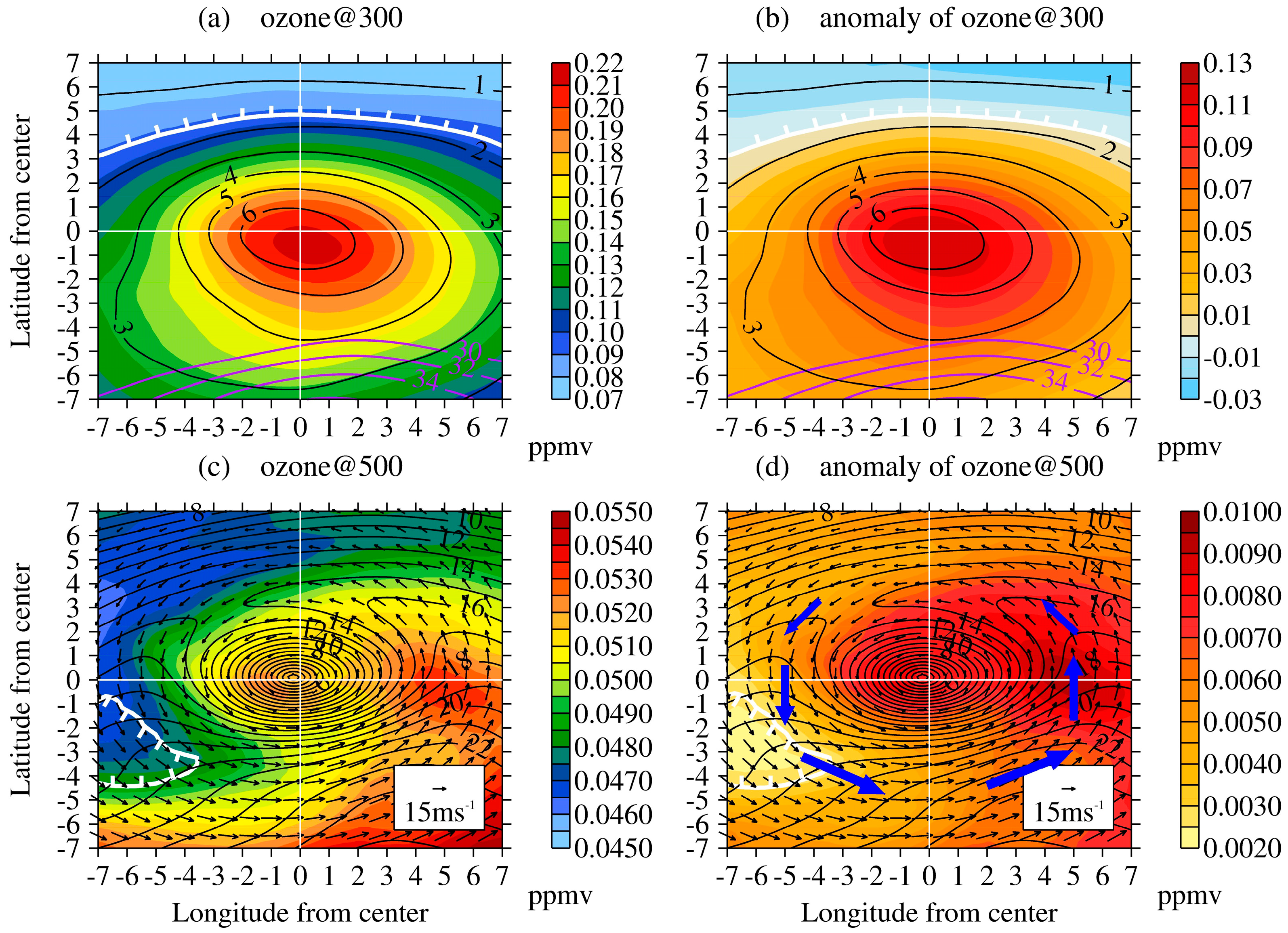
3.1. Ozone Spatial Distribution Revealed by the ERA-Interim Dataset

In the present study, we considered 300 and 500 hPa to be representative of the height of the upper and middle troposphere, respectively. Figure 3a,c show the synthetic spatial distribution of ozone concentrations in the research region (for a detailed description, see Appendix A) at the time when COLs reached their maximum intensity at 300 and 500 hPa, respectively. Figure 3b,d are the corresponding ozone anomalies (relative to the mean state over 11 years), which were used to further investigate the effect of COLs on increases in ozone concentration. To facilitate an analysis of the relationship between the distribution of ozone and the dynamic elements, data corresponding to the potential vorticity and jet stream of wind speed are superimposed on Figure 3a,b, and the horizontal wind vector and horizontal wind speed contours are superimposed on Figure 3c,d respectively.
The spatial distributions of ozone at 300 hPa clearly indicated a high PV area located around the center of the COLs, with a rich ozone area slightly southward of the center (Figure 3a). The maximum concentration of the ozone was 0.214 ppmv. The ozone anomalies shown in Figure 3b indicate that the area of a high positive anomaly also covered the center and southern part of the COLs. The stratospheric air intrusion caused by COLs resulted in an increase in the maximum ozone concentration of 0.119 ppmv relative to the average value over the 11-year period for the same region and height. There was a jet stream in the southern part of the COLs during their mature stage (Figure 3a,b). These characteristics show that, during the development of COLs, the role of the jet stream may cause downward movement and folding of the tropopause [34], and stratospheric air with a high ozone concentration is then transported downward. Therefore, an area with a high ozone concentration formed around the center and southern part of COLs.
In the middle troposphere (e.g., 500 hPa), the expected rich ozone area was also present around the center of COLs, but the range of concentrations was smaller than that at 300 hPa. In addition, we also identified another area of maximum ozone concentration east of the COLs (Figure 3c,d). This maximum ozone region was related to the horizontal circulation around the COLs. From the superimposed horizontal wind vector and wind speed contour in Figure 3c,d, we can see that the wind speed south of the COLs was stronger than that to the north due to the existence of a jet stream south of the COLs. In order to visually express this feature, we superposed the blue arrows in Figure 3d to show the anti-clockwise circulation and overall variation of wind speed. The length of the arrows represents wind speed. The wind speed distribution reveals that wind speed increases greatly in the direction of anticlockwise circulation in west periphery of COLs, while the opposite occurs on the east side. It results in the formation of wind divergence and convergence in the west and east of COLs, respectively. These indicated that the ozone does not accumulate under the wind divergence in the west of the COLs. The ozone is gradually transported eastward by the westerly wind south of the COLs and accumulates in the east due to the wind convergence, which increases the ozone concentration.
These spatial distribution characteristics of the ozone indicate that the increase in ozone concentration around the center of COLs is mainly related to downward movement of the tropopause or tropopause folding. Stratospheric ozone intrudes vertically into the troposphere and can reach the middle troposphere. The distribution of ozone in the middle troposphere is also related to the surrounding strong anticlockwise circulation of COLs. This distribution of ozone was explained by Li et al. [36]. They used a trajectory simulation to investigate the STE of a COL in June 2010. The results revealed that, during the COLs’ mature stage, the trajectory of the air mass gradually turned from a vertical rapid invasion in the upper troposphere into a relatively slow ‘rotary’ invasion in the middle troposphere.
The meridional and zonal cross sections of the ozone anomalies along the center of COLs shown in Figure 4 further illustrate that stratospheric ozone was transported downward as the tropopause descended, which resulted in an increased ozone concentration in the UTLS region. The superimposed PV and wind vector fields show that the PV isolines in the UTLS region formed a funnel shape and the 2 PVU isolines dipped as low as the surface of 450 hPa. Furthermore, the area with a large ozone positive anomaly corresponds to the funnel shape of the PV.
Figure 4 also reveals the asymmetric pattern of ozone anomalies. In meridional, positive ozone anomalies occurred south of the COLs from 600 to 70 hPa (Figure 4a). However, the vertical range (thickness) of positive ozone anomalies decrease sharply in the north of COLs, with negative ozone anomalies present above 400 hPa in the northern periphery of the COLs. Similarly, in the zonal region, positive ozone anomalies occurred west of the COLs from 600 to 80 hPa (Figure 4b). The thickness of positive ozone anomalies decreases gradually in the east of COLs, with negative ozone anomalies above 175 hPa in the eastern periphery of COLs. The reasons for this asymmetrical pattern of ozone may be related to the vertical motion and horizontal circulation. It can be seen from the superimposed wind vector that there was a significant ascending motion in the middle to upper troposphere to the north and east of the COLs, which prevents the downward transportation of the stratospheric ozone, and is even beneficial for the upward transport of air containing low ozone concentrations from the troposphere. Over the east of COLs, the maximum of positive ozone anomaly at 500 hPa (~ 0.01 ppmv), as shown in Figure 3d, can also be seen in Figure 4b. It is likely the positive effect from horizontal wind convergence exceeding the negative effect of ascending air at 500 hPa over this region and results in the zonal asymmetry here. In addition, the synthetic analysis selected the point with the lowest geopotential height at 500 hPa as the center of COLs, rather than using the geometric center point of the COLs, which likely also contributed to this asymmetric pattern.

3.2. Temporal Variations Revealed by the ERA-Interim Dataset

During the evolution of a COL, the ozone distribution exhibits different patterns in the UTLS region. The characteristics of ozone distribution in the different stages of COLs evolution are evaluated in this section.
Figure 5 shows the horizontal distribution of ozone anomalies in the research region at representative times of each stage at 300 hPa. As can be seen in the figure, variation in the ozone anomalies was closely related to the temporal evolution of COLs. In the pre-formation stage (Figure 5a), the maximum area of positive ozone anomaly was distributed mainly in the southwest portion of the COLs. As the COLs evolved from the pre-formation to the mature stage, the maximum area of the positive ozone anomaly gradually moved to the center of the COLs, while the ozone concentration and range gradually increased (Figure 5b,c). In the decay stage (Figure 5d), the increasing magnitude and extent of the ozone gradually decreased.
Figure 6 is the same as in Figure 5, but for 500 hPa. Figure 6 also indicates the relationship between variation in the ozone concentration and the evolution of COLs. The ozone anomaly gradually increased from the pre-formation stage to the formation stage (Figure 6a,b), and then gradually decreased until its decay (Figure 6c,d). Another important feature of Figure 6 is the anticlockwise rotation of the high ozone concentration region during the evolution of COLs. The ozone rotated from the south part of the COLs in the pre-formation stage (Figure 6a) to the southeast in the formation stage (Figure 6b) and then to the east in the mature stage (Figure 6c). This ‘rotating’ feature of the ozone during COLs evolution further demonstrates that the horizontal distribution of ozone at 500 hPa is related to the surrounding strong anticlockwise circulation of COLs. This is consistent with the ozone distribution patterns shown in Figure 3c,d which were caused by the ‘rotary’ invasion discussed in Section 3.1.
However, a comparison of Figure 5c and Figure 6c indicates a difference between 300 and 500 hPa in the ozone anomaly in the mature stage. At 500 hPa, there was no large positive ozone anomaly area, as there was at 300 hPa, and the ozone anomaly value was clearly weaker in the mature stage. One possible reason for this pattern of ozone variation could be the different transport mechanisms in the upper and middle troposphere. During the pre-formation and formation stages, the intensity of horizontal circulation in COLs is weak. Stratospheric ozone intrudes into the troposphere mainly by the rapid vertical transport caused by the descent or folding of the tropopause. The original vertical gradient of the ozone concentration was relatively large, which resulted in higher ozone concentrations at 300 and 500 hPa (Figure 5a,b, Figure 6a,b). As COLs evolved to the mature stage, the link with the jet stream is weaker, and the intensity of horizontal circulation at 500 hPa was enhanced. Therefore, the vertical inflow of stratospheric ozone-rich air into the COLs is inhibited, and the horizontal circulation plays a major role in this stage. Additionally, the horizontal gradient of the ozone concentration was small, which resulted in a minor increment in the ozone concentration at 500 hPa in the mature stage (Figure 6c).

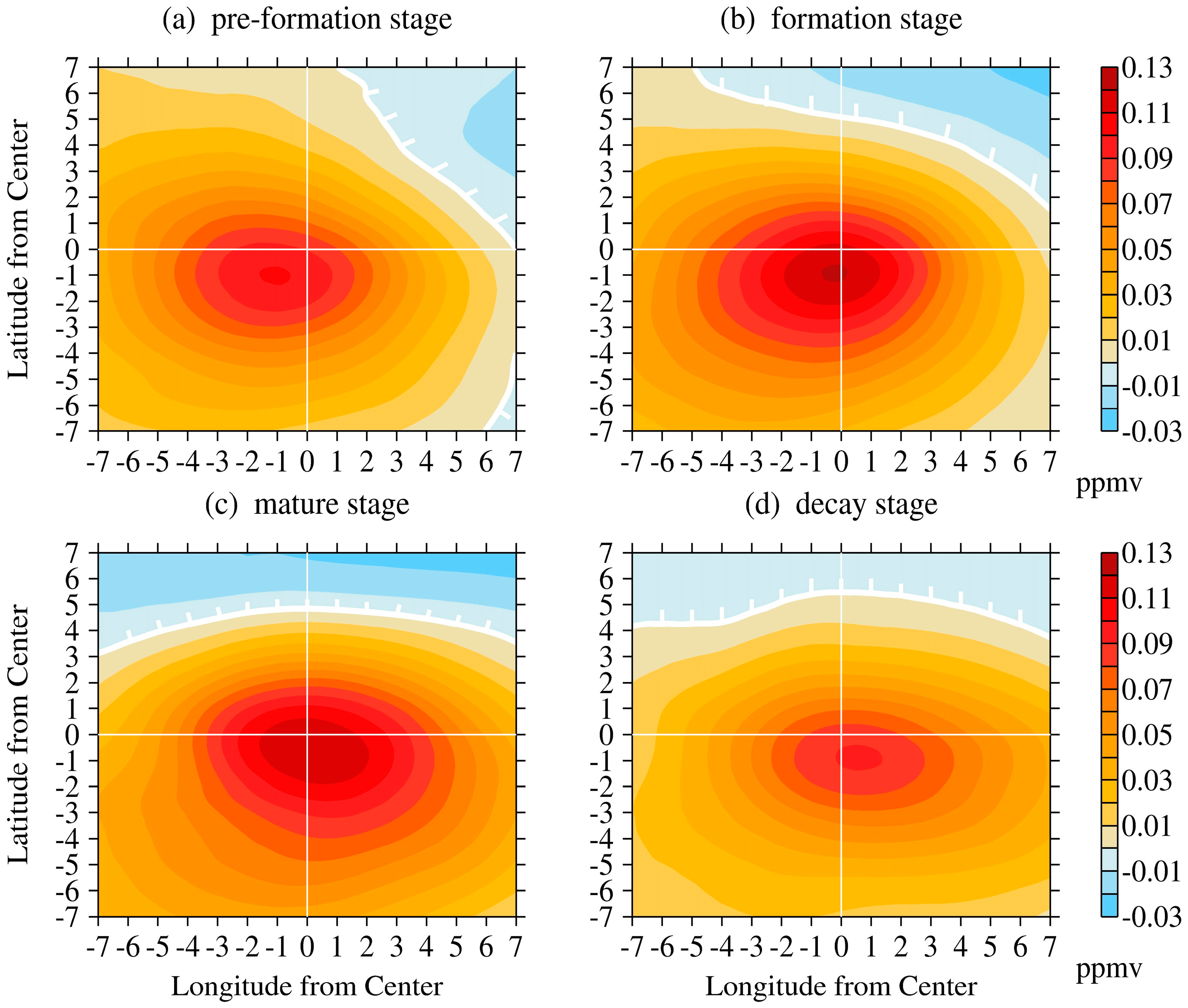
3.3. Temporal and Spatial Distributions Revealed by the AIRS Dataset

According to the method and process described in Section 2.4.2, we further investigated the characteristics of the spatiotemporal distribution of the ozone, as revealed by AIRS data. We also considered four representative times representing the four stages of COLs’ evolution.
Figure 7 and Figure 8 show the spatial patterns of the ozone during four stages of COLs near the tropopause (~300 hPa) and the middle troposphere (~500 hPa), respectively. Near the tropopause, when COLs were in the pre-formation stage, i.e., the formation and development of the trough, the figure shows a fan-shaped region of ozone distribution that corresponded to the shape of the trough (Figure 7a). High concentrations of ozone occurred in the northern part of the trough, with a maximum value of about 0.25 ppmv. McPeters et al. [48] found that the climatic annual average ozone concentration in the mid-latitudes (30°–60° N) and at a height of 9 km in the northern hemisphere is approximately 0.167 ppmv. This means that, during the pre-formation stage of the COLs (i.e., the development of the trough and ridge), there was an active ozone intrusion in the trough. This was consistent with our previous research that found active STE in the pre-formation stage of COLs [35]. In the formation stage of COLs (Figure 7b), the trough is cut off into an independent closed cyclone. The ozone is distributed mainly in the center and west of the COLs. With the evolution of COLs, the high ozone concentration region gradually moved to the center of the COLs. The ozone concentration in the center was higher than in the peripheral region, about 0.16 ppmv in the mature stage (Figure 7c), whereas, in the decay stage, the ozone concentration was significantly reduced (Figure 7d). These distribution patterns were consistent with our analysis, which are described in Section 3.2., where ERA-Interim data is used.
In the middle troposphere (Figure 8), the range and variation of the ozone concentration were also found to be linked to the life cycle of COLs. From the pre-formation to the mature stage, the enhanced ozone region gradually extended, and the concentration gradually increased, with a maximum value of about 0.13 ppmv. The climatic annual average concentration of ozone at this latitude and altitude is reportedly 0.0636 ppmv [48]. In the decay phase, the range and value of the ozone concentration were significantly reduced. Another prominent feature of the pattern of ozone distribution was the high ozone concentration region, which varied in the different stages of COLs evolution. The high ozone concentration region rotated anticlockwise around the center of COLs. As the COLs developed from the pre-formation to the decay stage, the enhanced ozone region was mainly concentrated in the northwest (second quadrant, Figure 8a), and then moved to the southwest (third quadrant, Figure 8b), to the south (third-fourth quadrant, Figure 8c), and, lastly, moved to the southeast (fourth quadrant, Figure 8d). This indicates that, during the development of COLs, according to the AIRS satellite data, the distribution of the ozone in the middle troposphere was affected by the surrounding strong anticlockwise circulation of COLs, which is consistent with the results revealed in the previous section using ERA-Interim data.
The statistical analyses of the AIRS and ERA-Interim data indicated a similar spatial pattern and variation in the ozone distribution in the UTLS region of COLs. The data consistently indicated that the horizontal distribution of the ozone in the middle troposphere was related to the circulation of COLs. However, a detailed comparison of the details also revealed some differences. The enhanced ozone region revealed by AIRS data (Figure 7c) was located relatively more northward than what was revealed by ERA-Interim data (Figure 3a). In addition, the ozone concentration shown by the AIRS data was higher than that from the ERA-Interim data. There are several reasons for these differences. First, due to the limitations of satellite scans, only part of the region of COLs could be captured (possibly due to high probability concentrated on the north of COLs), and the measurement times of AIRS and ERA-Interim data were not exactly consistent. Second, for a simple calculation, we used the central point defined at 500 hPa to determine the entire 3D grid. Although the difference between the central point of 300 hPa and 500 hPa is slight, it may also play a role in the discrepancies found between the ERA-Interim and AIRS analyses. In addition, there were also differences in the retrieval and assimilation methods used to acquire these data.

4. Summary and Discussion

Cut-off low systems are synoptic-scale patterns that play an important role in STE in the Ex-UTLS. Northeast Asia is an active region of COLs occurrence. To better understand these typical weather systems in key areas of STE over northeast Asia, we conducted a statistical analysis of the spatio-temporal distribution of the ozone in the UTLS region and assessed the STE process by using high-resolution ERA-Interim ozone data and AIRS ozone data.
The period of 2005–2015 was selected, and an automatic objective method was used to detect COLs in Northeast Asia. A total of 186 cases were obtained. Most COLs occurred in the late spring and early summer (May–June). An analysis of the PV showed that all cases had isolines of 2 PVU below the surface of 250 hPa, which indicates that the selected cases were accompanied by the invasion of stratospheric air into the UTLS region.
The statistical synthesis analysis of ozone concentration and ozone anomaly distribution obtained from ERA-Interim data showed that, in the mature stage of COLs, a rich ozone area was concentrated in the center of COLs at 300 hPa, which corresponded to the high PV area. At 500 hPa, there were two areas of a maximum ozone. One was expected and was located around the center of the COLs, but the main large-value area was located to the east of the COLs. This indicated that the ozone distribution in the upper troposphere was mainly affected by the descent or folding of the tropopause. In the middle troposphere, the redistribution of ozone was mainly affected by the anti-clockwise circulation of COLs and the patterns of the surrounding horizontal wind field. The vertical structure of the COLs showed that the PV isolines in the UTLS region displayed a “funnel” shape, and the 2 PVU isolines dipped as low as 400 hPa. The area of the ozone positive anomaly corresponded to the “funnel” pattern of PV.
The temporal variation in the ozone anomaly distribution revealed that the evolution of the ozone concentration was closely related to the lifecycle of COLs. It also clearly revealed that the redistribution of ozone at 500 hPa was mainly related to the anti-clockwise circulation of the COLs and the patterns of the surrounding horizontal wind field. We referred to this feature of ozone redistribution in the middle troposphere as “rotary” transport, as discussed in Li et al. [36].
The spatiotemporal patterns determined by the statistical analysis based on AIRS ozone data were overall consistent with those determined using ERA-Interim data. The results also clearly showed that the range and location of areas of high ozone concentration rotated anti-clockwise with the temporal evolution of the COLs. This further confirmed that the distribution of ozone in the middle troposphere was related to the surrounding horizontal circulation.
From the characteristics of the spatiotemporal ozone distribution, the process of ozone transport in the UTLS region could be inferred during the period of COLs evolution. First, in the upper troposphere and above, the STE was dominated by downward transport to the troposphere, which was caused by the descent or folding of the tropopause. This transport was usually relatively fast. In the middle troposphere (i.e., 500 hPa), the distribution of ozone was affected by the strong counter-clockwise circulation of the COLs and the surrounding horizontal wind field patterns. The ozone was relatively slowly transported (“rotary transport”) down to the low troposphere. The research we are conducting by the transport trajectory model initially revealed that these transport processes occurred over different time scales. Further study is needed in the future.
From a statistical perspective, this study revealed for the first time the spatiotemporal distribution of ozone in the UTLS region induced by COLs over Northeast Asia. The study has potentially identified the substance transport processes accompanying COLs in the UTLS region. It provides a foundation for understanding the overall effect of the weather system over Northeast Asia on the distribution of tracers in the UTLS region.

Author Contributions

Conceptualization, D.C. Investigation and methodology, D.C. and T.-J.Z. Formal analysis, software, and visualization, T.-J.Z. and L.-Y.M. Writing—original draft preparation, L.-Y.M. and L.C. Writing—review and editing, D.C. and C.-H.S. Supervision, D.G. All authors discussed the results and commented on the paper and figures.

Funding

This work was jointly supported by grants from the National Key Research and Development Project of China (2018YFC1505602), the National Natural Science Foundation of China (91837311, 41675039, 41875048, 41305038, 41575040), and College Student’s Practice Innovation Training Program of Jiangsu Province (201810300056Y).

Acknowledgments

We acknowledge the ECMWF for providing the reanalysis and ozone data. Furthermore, we would like to thank the team of the AIRS instrument for their continued effort in maintaining and continuously improving the AIRS data set. We thank S.-M.L. for English editing.

Conflicts of Interest

The authors declare no conflict of interest.

Appendix A. Statistical Synthesis Analysis of ERA-Interim Data

The analysis in Section 3.1 and Section 3.2 was conducted using a statistical synthesis method by the following four steps.
Step 1: Select a representative time for each stage of COLs evolution. In this step, we divided the lifecycle of a COL into four stages, according to the characteristics of COLs in Northeast Asia. These four stages were referred to as the pre-formation, formation, mature, and decay stages, and were similar to the upper-level trough development, tear off, cut off, and final stages described by Nieto et al. [16]. The 6-h ERA-Interim data at synoptic time steps was used for the division of the lifecycle. A representative time in each stage of all 186 COL cases was identified. Thus, a total of four representative times were determined for the whole lifecycle of a COL. The time of cut-off in a COL was the representative time in the formation stage of the COL, and the point 12 h before cut-off was the representative time in the pre-formation stage. The representative time in the mature stage was the time when the COLs attained their strongest intensity during the lifecycle. The point 12 h before the COLs disappeared was the representative time in the decay stage.
Step 2: Select an area as the research region for each COL. The objective region of each COL varied as the COL evolved, and it also differed from one event to the next. Thus, we selected a Lagrange viewpoint area as the research region that was constant for the different time periods and cases. Positioned at the central point of a COL, the 14° longitudes and 14° latitudes square area (extending seven latitudes and longitudes in four directions from the central point) was defined as the research region. The center point was determined as follows. When a COL undergoes the formation, mature, and decay stages, the point with the lowest geopotential height in the COL at 500 hPa was selected as the central point, and the lowest point in the inner ring of the trough was the central point during the pre-formation stage. In this way, the research regions of the 186 COL cases at each stage could be identified. This research region covered the main body of each COL. The ozone distribution within the region was discussed in Section 3.1 and Section 3.2.
Step 3: Synthetically calculate the average values of ozone and ozone anomalies for 186 cases. The values of ozone concentration and ozone anomalies in Section 3.1 and Section 3.2 are statistical synthetic averages of 186 cases. By taking the time when COLs reached their strongest intensity, the 14° longitudes and 14° latitudes research regions of the 186 COLs were coordinated based on the central point of each COL. Then, we calculated the average ozone concentration of 186 cases at each grid point in the research region. This provided the synthetic results of the average ozone field for the 186 COLs. Figure A1 show the synthetic results of the average ozone field for four representative times at 300 hPa as an example. The average ozone anomalies were obtained in the same way. First, the mean state of ozone over 11 years was calculated from the monthly average data from 2005–2015. Then, ozone anomaly values for each COL are calculated by subtracting the mean state of ozone from the ozone concentration in each COL research region. Lastly, the average ozone anomalies of 186 cases are synthetically averaged in the COLs coordinate. It is worth noting that both the ozone concentration and the ozone anomalies presented in the paper are calculated in the 186 COL events. This method was also used in the synthesis of other variable fields.
Step 4: The above synthetic analysis results were evaluated using a t-test.
Figure A1. The statistical synthesis ozone concentration (unit: ppmv) at 300 hPa in the research region at four stages: the pre-formation stage (a), formation stage (b), mature stage (c), and decay stage (d).
Atmosphere 10 00696 g0a1

Appendix B. Statistical Analysis of AIRS Ozone Data

In Section 3.3, our analysis was based on a method of matching footprints by the following steps. Due to the limitations of orbit scanning time and area, the evolution, the time period of each stage, and the central point of the COLs are all determined from ERA-Interim data.
Step 1: Divide the lifecycle of a COL into four stages. To discuss the variation in ozone distribution with the evolution of COLs, we divided the lifecycle of COLs into four stages, according to ERA-Interim data. This step was the same as the statistical analysis of ERA-Interim data described in Appendix A.
Step 2: Choose and match the AIRS footprints. All 186 events are involved in the matching of satellite footprints. We developed a simple algorithm to select and match the AIRS and ERA-Interim data. For each COL case and each stage of its evolution, the research region is defined as a circular region with a radius of 7° zonal distance (about 778.4 km and equivalent to ~10°–14° meridional distance, which vary with different latitudes) and the center point of the COLs as the center of the circle. If the footprints are within the research region based on the calculation of spherical distance and direction between the footprints and the circle center, they can be regarded as properly chosen.
Next, we assigned the matching footprints to the time grouping. The time period (24 h) of each stage was divided into four time groups, recorded as groups “a,” “b,” “c,” and “d,” respectively. For example, for a COL with a cut off at 06:00 on June 20, the time at 06:00, 12:00, and 18:00 on June 19, and 00:00 on June 20 corresponded to time groups a, b, c, and d, respectively, in its pre-formation stage. This method was applied in all cases to coordinate the time groups of each stage. In the process of the assignment, considering that the movement and intensity of COLs changed slightly over a short time, we neglected the time difference between the AIRS measurement time and the synoptic time of ERA-Interim data. We considered the time of footprints within the period 3 h before and after the ERA-Interim data time to be in the same group. For example, in the pre-formation stage of a case, the time of a matching sample point was at 08:48 on June 19, which was then assigned to 06:00 in group “a”. The temporal and spatial matching should both be reached to consider a sample point appropriate. The ozone concentration of selected points in the total COL events are marked with dots in Figure 7 and Figure 8. Due to orbit scanning limitations, not all four stages are captured for each COL by satellite. Therefore, the number of COLs captured at each stage is different. There are 116, 117, 123, and 118 cases captured in the four stages, respectively.

References

  1. Kremser, S.; Thomason, L.W.; von Hobe, M.; Hermann, M.; Deshler, T.; Timmreck, C.; Toohey, M.; Stenke, A.; Schwarz, J.P.; Weigel, R.; et al. Stratospheric aerosol—Observations, processes, and impact on climate. Rev. Geophys. 2016, 54, 278–335. [Google Scholar] [CrossRef]
  2. Solomon, S.; Rosenlof, K.H.; Portmann, R.W.; Daniel, J.S.; Davis, S.M.; Sanford, T.J.; Plattner, G.K. Contributions of stratospheric water vapor to decadal changes in the rate of global warming. Science 2010, 327, 1219–1223. [Google Scholar] [CrossRef] [PubMed]
  3. Yu, P.; Toon, O.B.; Bardeen, C.G. Black carbon lofts wildfire smoke high into the stratosphere to form a persistent plume. Science 2019, 365, 587–590. [Google Scholar] [CrossRef] [PubMed]
  4. Holton, J.R.; Haynes, P.H.; McIntyre, M.E.; Douglass, A.R.; Rood, R.B.; Pfister, L. Stratosphere-troposphere exchange. Rev. Geophys. 1995, 33, 403–439. [Google Scholar] [CrossRef]
  5. Stohl, A.; Wernli, H.; James, P.; Bourqui, M.; Forster, C.; Liniger, M.A.; Seibert, P.; Sprenger, M. A new perspective of stratosphere-troposphere exchange. Bull. Am. Meteorol. Soc. 2003, 84, 1565–1573. [Google Scholar] [CrossRef]
  6. Gettelman, A.; Hoor, P.; Pan, L.L.; Randel, W.J.; Hegglin, M.I.; Birner, T. The extratropical upper troposphere and lower stratosphere. Rev. Geophys. 2011, 49, RG3003. [Google Scholar] [CrossRef]
  7. Stohl, A.; Bonasoni, P.; Cristofanelli, P.; Collins, W.; Feichter, J.; Frank, A.; Forster, C.; Gerasopoulos, E.; Gäggeler, H.; James, P.; et al. Stratosphere-troposphere exchange: A review, and what we have learned from STACCATO. J. Geophys. Res. 2003, 108. [Google Scholar] [CrossRef]
  8. Pan, L.L.; Bowman, K.P.; Shapiro, M.; Randel, W.J.; Gao, R.S.; Canpos, T.; Davis, C.; Schauffler, S.; Ridley, B.A.; Wei, J.C.; et al. Chemical behavior of the tropopause observed during the Stratosphere-Troposphere Analyses of Regional Transport experiment. J. Geophys. Res. 2007, 112. [Google Scholar] [CrossRef]
  9. Pan, L.L.; Bowman, K.P.; Atlas, E.L.; Wofsy, S.C.; Zhang, F.; Bresch, J.F.; Ridley, B.A.; Pittman, J.V.; Homeyer, C.R.; Romashkin, P.; et al. The stratosphere-troposphere analyses of regional transport 2008 experiment. Bull. Am. Meteorol. Soc. 2010, 91, 327–342. [Google Scholar] [CrossRef]
  10. Guo, D.; Su, Y.C.; Zhou, X.J.; Xu, J.J.; Shi, C.H.; Liu, Y.; Li, W.L.; Li, Z.K. Evaluation of the trend uncertainty in summer ozone valley over the Tibetan Plateau in three reanalysis datasets. J. Meteorol. Res. 2017, 31, 431–437. [Google Scholar] [CrossRef]
  11. Guo, D.; Su, Y.C.; Shi, C.H.; Xu, J.J.; Powell, A.M. Double core of ozone valley over the Tibetan Plateau and its possible mechanisms. J. Atmos. Sol-Terr Phys. 2015, 130, 127–131. [Google Scholar] [CrossRef]
  12. Price, J.D.; Vaughan, G. The potential for stratosphere-troposphere exchange in cut-off-low systems. Q. J. R. Meteorol. Soc. 1993, 119, 343–365. [Google Scholar] [CrossRef]
  13. Shi, C.H.; Zhang, C.X.; Guo, D. Comparison of electrochemical concentration cell ozonesonde and microwave limb sounder satellite remote sensing ozone profiles for the center of the South Asian High. Remote Sens. 2017, 9, 1012. [Google Scholar] [CrossRef]
  14. Homeyer, C.R.; Bowman, K.P.; Pan, L.L.; Atlas, E.L.; Gao, R.S.; Campos, T.L. Dynamical and chemical characteristics of tropospheric intrusions observed during START08. J. Geophys. Res. 2011, 116, D06111. [Google Scholar] [CrossRef]
  15. Chen, D.; Chen, Z.Y.; Lü, D.R. Simulation of the generation of stratospheric gravity waves in upper-tropospheric jet stream accompanied with a cold vortex over Northeast China. Chin. J. Geophys. 2014, 57, 10–20. (In Chinese) [Google Scholar]
  16. Nieto, R.; Gimeno, L.; Torre, L.D.L.; Ribera, P.; Gallego, D.; García, J.A.; Nunez, M.; Redano, A.; Lorente, J. Climatological features of cutoff low systems in the Northern Hemisphere. J. Clim. 2005, 18, 3085–3103. [Google Scholar] [CrossRef]
  17. Zhang, C.; Zhang, Q.; Wang, Y.; Liang, X. Climatology of warm season cold vortices in East Asia: 1979–2005. Meteorol. Atmos. Phys. 2008, 100, 291–301. [Google Scholar] [CrossRef]
  18. Hu, K.X.; Lu, R.Y.; Wang, D.H. Seasonal climatology of cut-off lows and associated precipitation patterns over Northeast China. Meteorol. Atmos. Phys. 2010, 106, 37–48. [Google Scholar] [CrossRef]
  19. Gimeno, L.; Trigo, R.M.; Ribera, P.; García, J.A. Editorial: Special issue on cut-off-low systems (COL). Meteorol. Atmos. Phys. 2007, 96, 1–2. [Google Scholar] [CrossRef]
  20. Matsumoto, S.; Ninomiya, K.; Hasegawa, R.; Miki, Y. The structure and the role of a subsynoptic-scale cold vortex on heavy precipitation. J. Meteorol. Soc. Jpn. 1982, 60, 339–354. [Google Scholar] [CrossRef]
  21. Ancellet, G.; Beekmann, M.; Papayiannis, A. Impact of a cutoff development on downward transport of ozone in the troposphere. J. Geophys. Res. 1994, 99, 3451–3463. [Google Scholar] [CrossRef]
  22. Langford, A.O.; Masters, C.D.; Proffitt, M.H.; Hsie, E.Y.; Tuck, A.F. Ozone measurements in a tropopause fold associated with a cut-off low system. Geophys. Res. Lett. 1996, 23, 2501–2504. [Google Scholar] [CrossRef]
  23. Mohanakumar, K. Stratosphere Troposphere Interactions: An Introduction; Springer: Berlin, Germany, 2008; pp. 310–311. [Google Scholar]
  24. Yates, E.L.; Iraci, L.T.; Roby, M.C.; Pierce, R.B.; Johnson, M.S.; Reddy, P.J.; Tadić, J.M.; Loewenstein, M.; Gore, W. Airborne observations and modeling of springtime stratosphere-to-troposphere transport over California. Atmos. Chem. Phys. 2013, 13, 12481–12494. [Google Scholar] [CrossRef]
  25. Kuang, S.; Newchurch, M.J.; Burris, J.; Wang, L.H.; Knupp, K.; Huang, G.Y. Stratosphere-to-troposphere transport revealed by ground-based lidar and ozonesonde at a midlatitude site. J. Geophys. Res. 2012, 117, D18305. [Google Scholar] [CrossRef]
  26. Langford, A.O.; Brioude, J.; Cooper, O.R.; Senff, C.J.; Alvarez II, R.J.; Hardesty, R.M.; Johnson, B.J.; Oltmans, S.J. Stratospheric influence on surface ozone in the Los Angeles area during late spring and early summer of 2010. J. Geophys. Res. 2012, 117, D00V06. [Google Scholar] [CrossRef]
  27. Dempsey, F. Observations of stratospheric O-3 intrusions in air quality monitoring data in Ontario, Canada. Atmos. Environ. 2014, 98, 111–122. [Google Scholar] [CrossRef]
  28. Škerlak, B.; Sprenger, M.; Pfahl, S.; Tyrlis, E.; Wernli, H. Tropopause folds in ERA-Interim: Global climatology and relation to extreme weather events. J. Geophys. Res. 2015, 120, 4860–4877. [Google Scholar] [CrossRef]
  29. Vogel, B.; Pan, L.L.; Konopka, P.; Günther, G.; Müller, R.; Hall, W.; Campos, T.; Pollack, I.; Weinheimer, A.; Wei, J.K.; et al. Transport pathways and signatures of mixing in the extratropical tropopause region derived from Lagrangian model simulations. J. Geophys. Res. 2011, 116. [Google Scholar] [CrossRef]
  30. Škerlak, B.; Sprenger, M.; Wernli, H. A global climatology of stratosphere-troposphere exchange using the ERA-Interim data set from 1979 to 2011. Atmos. Chem. Phys. 2014, 14, 913–937. [Google Scholar] [CrossRef]
  31. Bian, J.; Gettelman, A.; Chen, H.; Pan, L.L. Validation of satellite ozone profile retrievals using Beijing ozonesonde data. J. Geophys. Res. 2007, 112. [Google Scholar] [CrossRef]
  32. Song, Y.; Lü, D.; Li, Q.; Bian, J.; Wu, X.; Li, D. The impact of cut-off lows on ozone in the upper troposphere and lower stratosphere over Changchun from ozonesonde observations. Adv. Atmos. Sci. 2016, 33, 135–150. [Google Scholar] [CrossRef]
  33. Liu, C.; Liu, Y.; Liu, X.; Chance, K. Dynamical and chemical features of a cutoff low over northeast China in July 2007: Results from satellite measurements and reanalysis. Adv. Atmos. Sci. 2013, 30, 525–540. [Google Scholar] [CrossRef]
  34. Shi, C.; Li, H.; Zheng, B.; Guo, D.; Liu, R. Stratosphere-troposphere exchange corresponding to a deep convection in warm sector and abnormal subtropical front induced by a cutoff low over East Asia. Chin. J. Geophys. 2014, 57, 1–10. [Google Scholar]
  35. Chen, D.; Lü, D.R.; Chen, Z.Y. Simulation of the stratosphere-troposphere exchange process in a typical cold vortex over Northeast China. Sci. China Earth Sci. 2014, 57, 1452–1463. [Google Scholar] [CrossRef]
  36. Li, D.; Bian, J.C.; Fan, Q.J. A deep stratospheric intrusion associated with an intense cut-off low event over East Asia. Sci. China Earth Sci. 2015, 58, 116–128. [Google Scholar] [CrossRef]
  37. Yang, J.; Lü, D.R. A simulation study of stratosphere-troposphere exchange due to cut-off-low over eastern Asia. J. Appl. Meteor. Sci. 2003, 27, 1031–1044. (In Chinese) [Google Scholar]
  38. Parkinson, C.L. Aqua: An earth-observing satellite mission to examine water and other climate variables. IEEE Trans. Geosci. Remote 2003, 41, 173–183. [Google Scholar] [CrossRef]
  39. Monahan, K.P.; Pan, L.L.; McDonald, A.J.; Bodeker, G.E.; Wei, J.; George, S.E.; Barnet, G.D.; Maddy, E. Validation of AIRS v4 ozone profiles in the UTLS using ozonesondes from Lauder, NZ and Boulder, USA. J. Geophys. Res. 2007, 112. [Google Scholar] [CrossRef] [Green Version]
  40. Kentarchos, A.S.; Davies, T.D. A climatology of cut-off lows at 200 hPa in the Northern Hemisphere, 1990–1994. Int. J. Climatol. 1998, 18, 379–390. [Google Scholar] [CrossRef]
  41. Nieto, R.; Sprenger, M.; Wernli, H.; Trigo, R.M.; Gimeno, L. Identification and Climatology of Cut-off Lows near the Tropopause. Ann. N. Y. Acad. Sci. 2008, 1146, 256–290. [Google Scholar] [CrossRef] [PubMed]
  42. Campetella, C.M.; Possia, N.E. Upper-level cut-off lows in southern South America. Meteorol. Atmos. Phys. 2007, 96, 181–191. [Google Scholar] [CrossRef]
  43. Wen, D.; Li, Y.; Zhang, D.L.; Xue, L.; Wei, N. A statistical analysis of tropical upper-tropospheric trough cells over the western north Pacific during 2006-2015. J. Appl. Meteorol. Clim. 2018, 57, 2469–2483. [Google Scholar] [CrossRef]
  44. Cao, F.; Gao, T.; Li, D.; Ma, Z.; Yang, X.; Yang, F. Contribution of large-scale circulation anomalies to variability of summer precipitation extremes in northeast China. Atmos. Sci. Lett. 2018, 19, e867. [Google Scholar] [CrossRef]
  45. Hoskins, B.J.; McIntyre, M.E.; Robertson, A.W. On the use and significance of isentropic potential vorticity maps. Q. J. R. Meteorol. Soc. 1985, 111, 877–946. [Google Scholar] [CrossRef]
  46. World Meteorological Organization (WMO). Atmospheric Ozone 1985: WMO Global Ozone Research and Monitoring Project Report; WMO 16; World Meteorological Organization (WMO): Geneva, Switzerland, 1986. [Google Scholar]
  47. Hoinka, K.P. Statistics of the global tropopause pressure. Mon. Weather Rev. 1998, 126, 3303–3325. [Google Scholar] [CrossRef]
  48. McPeters, R.D.; Labow, G.J.; Logan, J.A. Ozone climatological profiles for satellite retrieval algorithms. J. Geophys. Res. 2007, 112. [Google Scholar] [CrossRef] [Green Version]
Figure 1. Monthly distribution of the number (orange) and percentage (green) of 186 COL events.
Atmosphere 10 00696 g001
Figure 2. Percentage of COLs in which 1.6 or 2.0 PVU isoline dips below the barometric surfaces of the 200, 250, 300, 350, 400, 450, and 500 hPa, respectively.
Atmosphere 10 00696 g002
Figure 3. The statistical synthesis of the ozone concentration (a) and (c), unit: ppmv) and ozone anomalies (relative to the 11-year average ozone, (b), (d), unit: ppmv) in the research region at the time when COLs reached their maximum intensity at 300 and 500 hPa. The regions “downhill” of the white thick contour (in the direction of the ticks) did not meet the 95% confidence level following a t-test. Potential vorticity (black contour, unit: PVU) and jet stream (gray contour, >30 m/s, unit: m/s) superposed on 300 hPa, and the horizontal wind (vector) and horizontal wind speed (black contour, unit: m/s) superposed on 500 hPa. The horizontal axis is longitudinal from the center, and the vertical axis is latitudinal from the center. The origin is at the center point of the COLs.
Atmosphere 10 00696 g003
Figure 4. Meridional (a) and zonal (b) cross sections of the ozone anomalies along the center of COLs at the time of their maximum intensity. Potential vorticity (black contour, unit: PVU) and wind (vector, the synthesis of vertical and horizontal wind component) is superimposed on the figure. The regions “downhill” of the white thick contour did not meet the 95% confidence level following a t-test.
Atmosphere 10 00696 g004
Figure 5. The horizontal distribution of ozone anomalies (unit: ppmv) at 300 hPa in the research region at four stages: the pre-formation stage (a), formation stage (b), mature stage (c), and decay stage (d). The regions “downhill” of the white thick contour did not meet the 95% confidence level following a t-test.
Atmosphere 10 00696 g005
Figure 6. Same as Figure 5, but for 500 hPa.
Atmosphere 10 00696 g006
Figure 7. The horizontal distribution of ozone (unit: ppmv) near the tropopause (~300 hPa) in the pre-formation stage (a), formation stage (b), mature stage (c), and decay stage (d).
Atmosphere 10 00696 g007
Figure 8. Same as Figure 7, but for the middle troposphere (~500 hPa).
Atmosphere 10 00696 g008

