Prediction of Rainfall Using Intensified LSTM Based Recurrent Neural Network with Weighted Linear Units

Abstract

Prediction of rainfall is one of the major concerns in the domain of meteorology. Several techniques have been formerly proposed to predict rainfall based on statistical analysis, machine learning and deep learning techniques. Prediction of time series data in meteorology can assist in decision-making processes carried out by organizations responsible for the prevention of disasters. This paper presents Intensified Long Short-Term Memory (Intensified LSTM) based Recurrent Neural Network (RNN) to predict rainfall. The neural network is trained and tested using a standard dataset of rainfall. The trained network will produce predicted attribute of rainfall. The parameters considered for the evaluation of the performance and the efficiency of the proposed rainfall prediction model are Root Mean Square Error (RMSE), accuracy, number of epochs, loss, and learning rate of the network. The results obtained are compared with Holt–Winters, Extreme Learning Machine (ELM), Autoregressive Integrated Moving Average (ARIMA), Recurrent Neural Network and Long Short-Term Memory models in order to exemplify the improvement in the ability to predict rainfall.

1. Introduction

Rainfall is a major severe phenomenon within the climatic system. It has a straight influence on ecosystems, water, resources, management and agriculture. Rainfall is the main source for the people whose entire life depends on water. There are few states in India like Kerala, Karnataka, Goa, Orissa, West Bengal, Arunachal Pradesh, Sikkim and Uttarakhand that have heavy rainfall—around 3000 mm to 1500 mm per year—which helps farmers to cultivate their crops without bothering about the deficiency of water resources. But few other states like Uttar Pradesh, Rajasthan and Gujarat receive very low rainfall—less than 600 mm per year—which is a major cause for drought in those areas. Sometimes, heavy rainfall also leads to floods in states like Orissa and Kerala, which affects people by severely damaging their properties. As a result, the economy of these states goes down for a certain period, it takes a lot of time for the people to recover their original lifestyle and to carry out their occupation. Nearly 1400 people were dead due to flood in various places of India in the year 2018, so that leads to loss of human life too.

On the other hand, the major economy of a country depends on food production, which must be enough for the total population of the country; if so, then the dependency on other countries for the importation of food products is reduced. India receives 70% of the rainfall for irrigation during monsoon season, and due to increase in temperature and evapotranspiration, the water is not enough to use for the whole year for agriculture. Therefore, being aware of future rainfall becomes an important aspect of prediction and analysis of rainfall data that may help people find out a solution during deficit or surplus of rainfall.

Prediction of rainfall remains a severe concern and has grabbed the attention of industries, governments, risk management entities, and the scientific community as well. One main complex meteorological phenomenon is Rainfall. Rainfall is a random event, and the cause of its occurrence is very complex. Regarding weather predictions, among the climatic factors, even under similar weather conditions, there is a possibility that it might rain at this moment but not at another moment. Therefore, prediction becomes crucial to gain knowledge of the atmosphere’s condition. Predictive Analytics is an innovative analytics scheme to perform such forecasting and predict actions on future events and happenings using the previous datasets. It is a factor of climatic condition through which numerous human activities such as power generation, construction, agricultural production, tourism and forestry among others are affected [1]. Traditional forecasting of weather conditions reminds about meteorologists making predictions in view of their experience by sitting with weather charts spread in front of them. This experience is the knowledge gathered from years of observations and from background on weather theory [2]. To this extent, rainfall prediction is vital since this variable is the one that has maximum correlation with adverse natural events like landslides, flooding, mass movements and avalanches. These incidents have affected society for years. This appears to be the main motivation for the evolution of numerical weather prediction and weather prediction by machine learning algorithms.

One application of science and technology to forecast the atmosphere’s state for the provided location is rainfall forecasting. It includes numerous techniques like statistics, data mining, modelling, artificial intelligence and machine learning. Real-time and accurate rainfall prediction has remained a major challenge for many decades because it is nonlinear and stochastic in nature. Thus, having a suitable approach for the prediction of rainfall makes it possible to take preventive and mitigating measures for all these naturally occurring phenomena. Several methods for predicting rainfall were employed in the past [3]. The two fundamental approaches to predicting rainfall are the dynamical and the empirical approach. In the dynamical scheme, predictions are carried out by physically built models that are based on the equations of the system that forecast the rainfall. As an approach to forecast weather conditions of by such numeric means, meteorologists have developed systems that approximate temperature change, pressure change, etc., using mathematical equations. The Empirical method is based on the analysis of past weather data and their relationship with various atmospheric variables over diverse regions. The most commonly employed empirical approaches are regression, fuzzy logic and deep learning techniques.

Artificial Neural Networks (ANN) play a major role in prediction, and an appropriate neural network model has to be chosen based on the nature of data taken for analysis. There are many categories of neural networks like feed forward neural networks, neural networks with back-propagation, recurrent neural networks, etc., where each model has its unique way of prediction approach. To deal with rainfall data, recurrent neural networks are the better option since they can handle time series data efficiently. Even unexpected heavy rainfall can be predicted by multilayer perceptron which is expressed as “guerrilla rainstorms” in Japan [4]. Back-propagation has an important part in prediction since the neurons perform predictions by remembering the weights applicable for every range of input. By using such scenario, monthly rainfall prediction is carried for the Kalimantan region in Indonesia using Back-propagating Neural Network (BPNN) with least error [5].

Fuzzy logic is also one of the methods used for many years, especially in weather data for various predictions. Rainfall prediction is not only carried out in terms of numerical scale, but it was also labelled as high, medium and low using fuzzy logic based on the correlated variables like temperature and wind speed and processed using triangular membership functions [6]. The likelihood of rainfall is predicted in a better way using fuzzy logic, compared to two logic levels since many real time problems rely on several factors [7]. Similarly, Support Vector Regression (SVR) is used to forecast flash floods in mountainous catchments in China; for different phase lags which commenced one to three hours ahead, forecasting produced satisfactory results [8]. Our previous work also clearly talks about the statistical forecasting methods used for prediction [9].

Some problems commonly faced by prediction methods are the insufficient capacity of memory occurrence of vanishing gradient in the network, increased prediction error and modeling a system that gives accurate forecast of rainfall. In this paper, Intensified LSTM based RNN is modeled as the prediction network to overcome capacity insufficiency by employing LSTM network, to mitigate the vanishing gradient by multiplying input sequence to the layers of LSTM, to reduce the prediction error and to provide accurate prediction of rainfall by using Adam Optimizer. Hence, this model mainly focuses on mitigating the problems faced by the existing methods of predictive analysis, thereby developing an efficient model for prediction.

The organization of the research paper is as follows: Section 2 includes the work related to the existing systems. Section 3 includes the Research methodology and the framework for the proposed system. Section 4 includes the results and discussions for the proposed system. Section 5 presents our conclusion and a scope for the future work.

2. Experiments

Many researchers have worked on the predictive analysis of rainfall. Some studies are discussed in this section. There are two approaches for predicting rainfall; they are the statistical approach and machine learning approach. Traditional models for the prediction of rainfall employed statistical methods. Holt–Winters algorithm is one such method. Variants of Holt–Winters algorithm have been recommended by several papers. Improved method of prediction using additive Holt–Winters was discussed in [10], which is approximately 6% more accurate than the Multiplicative Holt–Winters method. It is a big data approach in which the average measure of the sequence in the past is computed in this predictive algorithm. However, the datasets taken are in a controlled range.

In [11], the maximum and minimum temperature time series of the region was predicted by employing Holt–Winters method which was implemented for Junagadh region using Excel spread sheet. Triple exponential smoothing technique is performed, and the performance of the methodology is measured by three parameters, MSE, MAPE and MAD. Processing huge dataset in Excel spreadsheet is not an easy task and therefore this method is suitable for smaller datasets. In [12], the additive Holt–Winters method was utilized for the analysis of rainfall series of river catchment areas. The model predicts the rainfall and then the predictive and actual data are sent as input to the undesirable model for the purpose of evaluating the performance of the model.

Another statistical approach for prediction algorithm is the ARIMA model and is used for Non-stationary time series applications. Such a model was discussed in the papers [13,14,15]. Reference [13] focused on the generation and prediction of time series values of only rain attenuation, whereas [14] described Box Jenkins time series seasonal ARIMA model for predicting rainfall on seasonal basis. Generally, ARIMA models are used for modelling hydrologic and geophysical time series data. One main issue in such modelling processes is the identification of the order of the models and so [15] focused on model identification of hydrological time series data. However, this ARIMA model assumes that the data are stationary and so its ability to capture non-stationary data is very limited. Therefore, the statistical methods are applicable only to the linear applications. This is considered as one of the main drawbacks to use statistical methods when it comes to non-linear and non-stationary applications.

In [16], the prediction of rainfall was carried out by employing data mining algorithms such as Logistic Model Tree (LMT), Random Forest (RF) and Classification and Regression Tree models (CART). These were analyzed comparatively, and it was concluded that Random Forest shows superiority over other methods and exhibits a success rate of 0.83. However, these models require constant evaluation on the information because the related factors change dynamically. Modelling and prediction of rainfall using data mining approach was carried out in [17]. In this paper, radar reflective and Temperature data are considered. Five data mining schemes were employed, namely, random forest, neural network, support vector machine, k-nearest neighbor, regression tree and classification. Among these techniques, Multi-Layer Perceptron (MLP) neural network was found to perform better than the rest. However, the drawback in MLP is that it consumes a long time for convergence, which depends on the initial values and minimization algorithm being applied.

Functionalities of data mining like clustering, regression and classification, were employed by the authors of [18]. They classified the reasons why rain falls at the ground level. The values of rainfall were computed using five years of input data by using Pearson correlation coefficient, and the rainfall was predicted for future years by multiple linear regression technique. However, the predicted values lie below the actual values, thereby showing approximate values instead of accurate ones.

As a neural network model, Multi-Layer Perceptron (MLP) was developed using a hybrid algorithm incorporating Back-propagation (BP) and Random Optimization (RO) methods, and Radial Basis Function Network (RBFN) with the Least Squares Method (LSM) was carried out in the process of predicting rainfall in [4]. The comparison was shown with two other models in the paper. Prediction was based on the volume of the rainfall at different time scales, so the accuracy varies with respect to the precipitation level. A K-nearest-neighbor (KNN)-based non-parametric non-homogeneous hidden Markov model was developed in [19] and applied for spatial down scaling of multi-station daily rainfall occurrences. However, models that are developed based on KNN algorithm re-sample the rainfall at all the locations with replacements on the same day, thereby resulting in less efficient responses.

Rainfall prediction was processed using China Meteorological Administration (CMA) open dataset [20]. Methods considered for comparison were Naïve Bayes, Back-propagation Neural Network and Support Vector Machine. This approach is suitable for linear applications and so accurate prediction for non-linear dataset is difficult using this technique. Artificial intelligence methods such as Single Layer Feed-Forward Neural Network (SLFN) were carried out in [21] for the prediction of rainfall.

Feed-forward neural networks are computationally faster since weight tuning is not needed, thus they works well for large datasets [22]. But a major drawback is, they do not take the previous state of prediction into account which is an important characteristic for time series data so the accuracy is lowered. Hence, we are motivated to build a system that takes previous data into account; one such system is Recurrent Neural Network (RNN). Recurrent Neural Network was modeled for the early detection (prediction) of cases dealing with heart failure and controls by the use of Gated Recurrent Units (GRUs) in [23]. Performance measures were compared with neural network, K-Nearest Neighbour, logistic regression and Support Vector Machine. This paper enhances the importance of taking sequential datasets for prediction algorithms.

A forecast model for proactive cloud auto-scaling models combining with few mechanisms was built in [24]. Multivariate Fuzzy-LSTM (MF-LSTM) was modeled for the forecast of consumption of resources with data of multivariate time series simultaneously. This system was verified using Google trace data to validate its feasibility and efficiency when applied to clouds. However, this LSTM network does not try to lessen the vanishing gradient problem. LSTM based Differential RNN (dRNN) was modeled in [25] where the significant spatiotemporal dynamics were considered. Derivatives of States (DoS) were used in dRNN. This method is not designed for crowd scene analysis and it does not provide an end-to-end solution.

Several other LSTM variants were suggested to enhance the architecture of standard LSTM. Bidirectional LSTM [26] grasps both previous and future contexts of the input data. Bidirectional RNNs are designed for input sequences whose start and end points are known. Therefore, these methods are not suitable for unknown input datasets. Multidimensional LSTM (MDLSTM) [27] extends the memory of LSTM throughout every N-dimension using the internal connections from the previous cell state. Grid LSTM [28] provides a solution by altering the computation of output memory vectors. Although the above-mentioned variants of LSTM show superiority in some respects, these papers did not consider the mitigation of vanishing gradient as a concern. A system that mitigates the vanishing gradient is modeled in our proposed system using a sigmoid activation function multiplied with the input in the input gate and a tanh activation function multiplied with the input in the candidate layer of LSTM.

3. Methodology

The methods for the prediction of rainfall can be basically categorized into two types, classic statistical algorithms and machine learning algorithms. Statistical algorithms are the conventional algorithms employed for the prediction of rainfall. Statistical methods are applicable for linear applications, whereas machine learning algorithms are applicable for non-linear applications such as prediction of rainfall. In machine learning algorithms, neural networks are of two types, namely, Feed Forward Neural Networks (FFNN) and RNN. Neural networks employed in feed forward structure are not suitable for the prediction of rainfall since they do not take previous state into account. RNN on the other hand has shorter memory to hold long back status of the datasets. Hence, we go for RNN in combination with Long Short-Term Memory. The Intensified LSTM developed in this research work can hold a large number of previous datasets, thereby mitigating vanishing gradient, which leads to better accuracy in prediction.

3.1. Recurrent Neural Networks

The prediction of cumulative measures from the sequences of vectors of variable-length including a component ‘time’ is extremely significant in machine learning. RNN has the power of learning previous-term dependencies. Previous-term dependencies are very much essential when it comes to predicting weather patterns. RNN is useful in that perspective since it is an artificial neural network utilized especially for developing prediction networks using long-term time series dataset. The general RNN performs prediction at a time t as follows,

$$H_t=g(W_h\left[H_{t-1}, X_t\right]+b_h)$$

(1)

$$O_t=f\left(W_o\ast H_t+b_o\right)$$

(2)

where H_t is the hidden state, O_t is the predicted output, W_h and W_o are the weights assigned in hidden layer and output layer, b_h and b_o are the bias for hidden and output layer, g is the activation function used in hidden layer and f is the output function for prediction. Prediction performance of RNN majorly depends on the activation function, which takes the current input and previous state as input vector and predicts output based on the hidden state result. Based on this model, much research work has been carried out with certain improvements in the model as discussed in related work section.

Elman network is a category of RNN comprising one or many hidden layers. The first layer contains the weight vectors that are attained from the input layer. Every layer receives weight from the previous layer [29]. RNNs are designed to capture temporal contextual information along time series data. Unlike the traditional FFNNs, RNNs possess feedback loops in their structure which are used for feeding outcome of the preceding time steps as input to the current time step. This construction enables RNNs to develop complex temporal contextual figures along time series dataset.

Usually the change in weight ($\Delta$) during back-propagation in a neural network is calculated based on the error (E) occurred for the weight (W) assigned in the previous state as follows,

$$\Delta =\frac{\partial E}{\partial W}$$

(3)

The Back-Propagation Through Time (BPTT) is a technique that is generally used for training the RNNs, which adjusts the weight of the network to reduce the error by back-propagating to certain count of states n constantly, and finally, the summation of error to the respective weights of the back-propagated states are calculated for the change in weight as,

$$\Delta ={{\displaystyle \sum }}_{i=1}^n\frac{\partial E_i}{\partial W_i}$$

(4)

The partial derivatives of the Recurrent Neural Networks for n number of states is represented as,

$$\frac{\partial E}{\partial W}=\frac{\partial E}{\partial W_1}+\frac{\partial E}{\partial W_2}+\dots +\frac{\partial E}{\partial W_n}$$

(5)

Nevertheless, it is challenging to train the traditional RNNs using BPTT because of the exploding and vanishing gradient problems. Errors from later time steps are difficult to propagate back to previous time steps for appropriate changes inf network parameters. To address this problem, the LSTM unit has been developed by reducing the loss at every stage significantly.

3.2. Role of Activation Functions

As specified in the previous section, activation functions are the major cause for the prediction and entire network performance. Hence, choosing the activation function is a major challenge for a suitable application. Assigning and adjusting the weights for the activation function has a great impact on the results of activation functions since the neurons learn the relationship between input vector and output based on the weight tuning. During the training phase, the difference in change of weights is high at the initial stage due to high learning rate, it gradually decreases and learning stops when the weight is nearest to zero, which conveys there is no change in output for the change in input. The relationship between weight update W_t and learning rate Lt at a time t is given as

$$W_t=L_t\times E_w$$

(6)

Weight tuning helps the neural networks to restyle the steepness of the curve whereas bias value applied to the network finds the best fit for the curve jointly with the data through shifting.

Many activation functions have been developed in recent years, but the most commonly used activation functions are sigmoid, tanh and Relu. Every activation function has its own pros and cons, so let us discuss them in detail. Sigmoid is the function habitually used for hidden layers of Artificial Neural Networks which maps any range of input values between 0 and 1. The function squashes even a large input values to a small range due to which a substantial change in input reflects as a small change in output. Therefore, this function can be used for those applications that need to compute probability as outcome, and it is represented as below,

$$f\left(x\right)=\frac{1}{1+e^{-x}}$$

(7)

During back-propagation, the gradient of the function decreases exponentially, which leads to very small derivatives and weight tuning in the initial layers of the neural network. This is defined as vanishing gradient problem, in which the neurons tend to stop learning at a certain level. The derivative of the sigmoid function is

$$\frac{d\left(f\left(x\right)\right)}{dx}=\frac{e^x}{{\left(1+e^x\right)}^2}$$

(8)

One more important issue in the sigmoid function is that the sigmoidal curve is not centered to the origin; instead, it is centered by 0.5. Thus computations related to transitions are difficult in the curve, and the usage of the tanh function is loftier than sigmoid. Tanh activation function also called hyperbolic tangent is more eminent than the sigmoid in several ways. It accepts a wide range of inputs such that the function ranges between −1 and +1, thereby computing the output for negative inputs also. The tanh function is defined as

$$f\left(x\right)=\frac{e^x-e^{-x}}{e^x+e^{-x}}$$

(9)

For this reason, the hyperbolic tangent curve is steeper than the sigmoidal curve, and hence, derivatives are sturdy, which minimizes the vanishing gradient compared to the sigmoid. The derivative of hyperbolic tanh is

$$\frac{d\left(f\left(x\right)\right)}{dx}=1-{\left(f\left(x\right)\right)}^2$$

(10)

When moving onto deeper networks, vanishing gradient problem still occurs in tanh function. Thus, the search for a better activation function to mitigate the gradient problem led to the utilization of a Relu (Rectified Linear Unit) activation function by many researchers recently. The Relu function uses only two simple constraints, which is easier to implement as given below,

$$f\left(x\right)=\{\begin{array}{c}0 for x<0\\ x for x\ge 0\end{array}$$

(11)

The above defined Relu function enlarges its range as [0 to ∞], which is comparatively higher than the sigmoid and tanh functions. It maps all the negative values as 0 and other values as x due to which even small input values reflects a significant change in output also. Examining the derivatives of Relu, it is 1 for all x greater than 0 and 0 for x less than 0, but if x is 0, then derivative never exist.

$$\frac{d\left(f\left(x\right)\right)}{dx}=\{\begin{array}{c}1 for x>0\\ 0 for x<0\\ not exist for x=0\end{array}$$

(12)

Due to this possession, Relu can withstand by mitigating vanishing gradient with better learning rate for all x values. However, there is an issue with the Relu activation function; as mentioned in the Equation (12), all the negative values of x are mapped to zero, which prevents the network to stop learning, which would lead the neurons to die after certain number of continuous inputs with no gradient. Even if one of the input values tends to achieve the gradient among many consecutive negative values or zeros, the network can sustain by itself and learning continues since neurons are alive. This issue is addressed in Intensified LSTM in Section 3.4.

3.3. Long Short Term Memory

A specific architecture of RNN is LSTM, which was an intended design for modelling temporal sequences. LSTM has a long-range dependency that makes it more accurate than conventional RNNs. Back-propagation algorithm in RNN architecture causes error backflow problem [30]. The fundamental idea behind the algorithm of back-propagation is the composite function chain rule. Stochastic Gradient Descent (SGD) is an efficient algorithm to search for the local minimum of the loss function. Once we attain the gradients from the internally existing nodes of the computational graph, we can get the gradients of the nodes with a starting point, by calculating the gradient of that point and searching in the direction of a negative gradient. This is the fastest way we search for a local minimum.

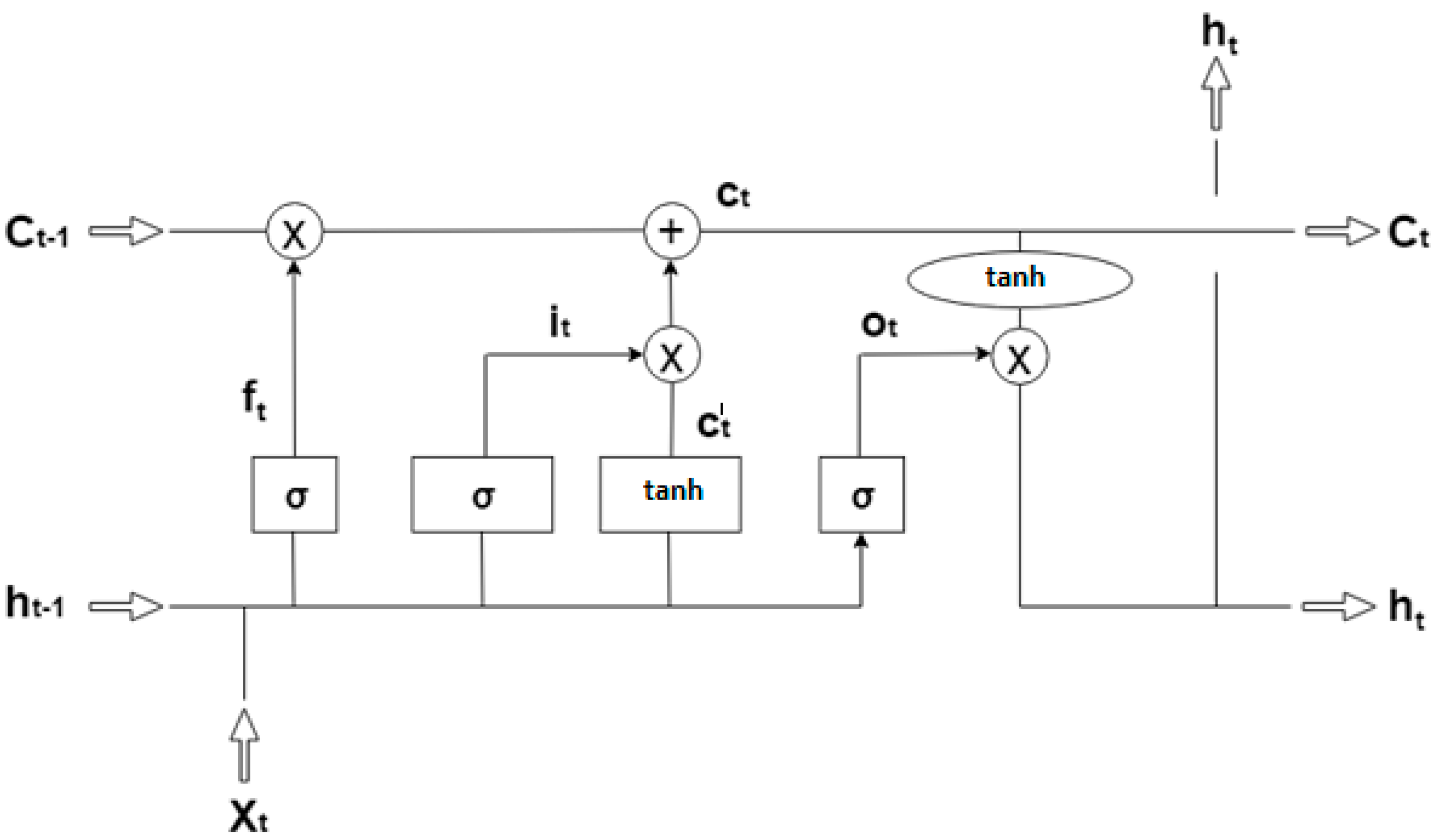
The basic structure of LSTM is known as a memory cell for remembering and propagating unit outputs explicitly in different time steps. For remembering the information of temporal contexts, the memory cell of LSTM utilizes cell states. It also has a forget gate, an input gate and an output gate, to control information flow between different time steps. In this study, neural networks based on LSTM were employed to forecast background radiation from the time-series weather data. The mathematical challenge in learning the long-term dependencies in the structure of recurrent neural networks is called as the problem of vanishing gradient. As the length of input sequence increases, it becomes harder to capture the influence of the earliest stages. The gradients to the first several input points vanish and become equal to zero. The activation function of the LSTM is considered as the identity function with a derivative of 1.0, due to its recurrent nature. Therefore, the gradient being back propagated neither vanishes nor explodes but remains constant.

A node’s activation function defines the output of that particular node as discussed in Section 3.2. Activation functions that are commonly used in LSTM network are sigmoid and hyperbolic tangent (tanh). The actual architecture of LSTM proposed is implemented with the sigmoid function for forget gate and input gate and with the tanh function for candidate vector that updates the cell state vector [30]. These activation functions of LSTM are calculated for Input gate $I_t$, Output gate $O_t$, Forget gate $F_t$, Candidate vector ${C^{\prime }}_t$, Cell state $C_t$, and Hidden state $h_t$, using the following formulae,

$$I_t=sigmoid\left(W_i\left[X\left(t\right),h_{t-1}\right]+b_i\right)$$

(13)

$$F_t=sigmoid\left(W_f[h_{t-1},X\left(t\right)\right]+b_f)$$

(14)

$$O_t=sigmoid\left(\left(W_o[h_{t-1},X\left(t\right)\right]+b_o\right)$$

(15)

$${C^{\prime }}_t=tanh\left(W_c\left[h_{t-1},X\left(t\right)\right]+b_c\right)$$

(16)

$$C_t=F_t\ast C_{t-1}+I_t\ast {C^{\prime }}_t$$

(17)

$$h_t=O_t\ast \tan \mathrm{h}\left(C_t\right)$$

(18)

where X(t) is the input vector, $h_{t-1}$ is the previous state hidden vector, W is the weight and b is the bias for each gate. The basic structural representation of LSTM network is shown in Figure 1.

3.4. Intensified Long Short-Term Memory

The actual LSTM architecture uses sigmoid and tanh functions as explained in previous section, but there are various concerns about the activation functions used by LSTM. These difficulties were also explained in the previous section. To avoid the vanishing gradient problem, it is necessary to hold the gradient to certain levels of back-propagation, and thereby learning continues with neurons active throughout the training phase. Sigmoid weighted linear units are proposed [31] to handle the gradient problems that occur in back-propagation, which multiply the input value to the sigmoid activation function. Having this as a core idea, Intensified LSTM was developed.

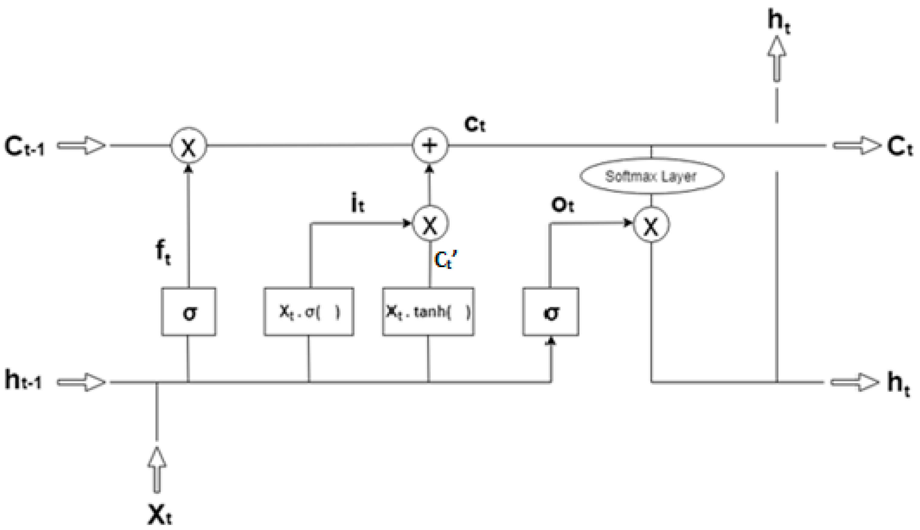
Cell state is a space that is specifically designed for storing past information, i.e., the memory space. It mimics the way the human brain operates when making decisions. Operation is executed to update the old cell state. This is the time where we actually drop old information and add new one. Three sigmoid functions (forget gate, input gate, output gate) and two tanh functions (candidate vector and output gate) are used by actual LSTM, but multiplying the input value with forget gate and output gate is not serviceable since the forget gate decides to keep the current input or not and the output gate yields the predicted value, which is already processed using cell state information. Hence, it is clear that input gate and candidate vector play a major role in updating the cell state vector from which the LSTM learns the new information and analyses to predict the output value based on the current input. Based on this, the input value is multiplied with the sigmoid function in input gate and tanh function in candidate vector. The structural representation of the proposed Intensified LSTM is displayed in the Figure 2. It is clear that LSTM has a more complex structure to capture the recursive relation between the input and hidden layer. The output $h_t$ can be obtained, same as that of a regular RNN. The proposed Intensified LSTM contains the following components,

• Input Gate “I” (with sigmoid activation function multiplied by the input);
• Forget Gate “F” (with sigmoid activation function);
• Candidate vector “C’” (with tanh activation function multiplied by the input);
• Output Gate “O” (with Softmax activation function);
• Hidden state “h” (hidden state vector);
• Memory state “C” (memory state vector).

All the gate inputs and layers inputs are initialized. X(t) (current input) is the input sent into the memory cell of LSTM, $h_{t-1}$ (previous hidden state) and $C_{t-1}$ (previous memory state). The layers are single layered neural networks with the sigmoid function multiplied by its input as activation function in the input gate, tanh multiplied by its input is taken as activation function for candidate layer, sigmoid is taken as activation function for the forget gate and Softmax regression function for computing the hidden state vector. With the help of the forget gate, the influence of current input over the previous state is analyzed and decides whether the current input needs to be stored in cell state or not (data is stored through input and candidate vector). If not needed, then the sigmoid function produces 0, which deactivates the forget gate; if needed, it then produces 1 to activate the gate as in Equation (19). Based on this decision, all the other gates in LSTM are activated or deactivated for certain input.

$$F_t=\{\begin{array}{ll}1& store the data\\ 0& discard the data\end{array}$$

(19)

When it is decided to keep the current input, the network seek to learn the new information carryover by the current input by comparing it to the previous state. The previous state vector $h_{t-1}$ contains the knowledge about all previous inputs and the corresponding change in output for various input vectors. Based on this, the sigmoid function in the input gate is processed first that leads to a value between 0 and 1 which depicts the range of new information available in the current input and the obtained value is multiplied by the input value as in Equation (20). Now the range of value produced is [0,∞] at the input gate, which in turn avoids the vanishing gradient for the same range of values in the input vector, thereby empowering the network to learn from every input.

$$I_t=X\left(t\right)\times sigmoid\left(W_i\left[X\left(t\right),h_{t-1}\right]+b_i\right)$$

(20)

With respect to the candidate gate C′, tanh function is activated using the current input and previous hidden state, which produces a value between −1 and +1 that illustrates the contemporary data to be updated in the cell state vector. This obtained value is multiplied with current input as in Equation (21) which produces candidate vector lying between [−∞,+∞], which in turn improvises the learning to update the new information in cell state vector for an even smaller change in time series.

$${C^{\prime }}_t=X\left(t\right)\ast tanh\left(W_c\left[h_{t-1},X\left(t\right)\right]+b_c\right)$$

(21)

The above mentioned technique has the advantage of self-stabilization so that it reduces the rate of propagation, and the global minimum, where the derivative is zero, functions as a soft floor on the weights, which in turn functions as regularizer implicitly inhibiting the learning of weights for large magnitudes. Hence, there is always a gradient network that learns the new information by minimizing the data loss and the error produced by the network.

Softmax regression computes the probability distribution of one event over n different events. The computed probability distribution can be used later for finding the target output for the inputs given. Outputs from the memory cell of LSTM are $h_t$ (current hidden state) and $C_t$ (current memory state). The mathematical formulae for the output gate and hidden state of Intensified LSTM are given in the following manner.

$$O_t=softmax\left(W_o[h_{t-1},X\left(t\right)\right]+b_o)$$

(22)

$$h_t=O_t\ast softmax\left(C_t\right)$$

(23)

The output layers compute all the processed outputs and the iteration continues until the error value of the hidden value results to zero.

Performance metrics considered for the validation of the proposed prediction model are RMSE, losses, learning rate, and accuracy. LSTM exhibits a major advantage in extending the memory capacity of the neural network. This leads to holding a huge dataset of rainfall background as a reference for the forecasting system. Holding a large number of data may have a great impact on the accuracy of prediction. As the layers use activation functions to produce the output of the fundamental unit of the neural network, which is the neuron, the gradients of the loss function approach zero, making the network tedious to train. The objective of mitigating this vanishing gradient problem is achieved by multiplying input data sequences to the activation functions of input gate and candidate layer. Upon mitigating the vanishing gradient, the time taken to train the network is reduced. This reduction in time causes high learning rate, thereby reducing the losses. The impact on learning rate and losses automatically causes the RMSE value to decrease.

The non-rainy days are taken as zeros in rainfall dataset. Due to the presence of the zeros in the rainfall data, RMSE calculated for the rainfall prediction models is higher when compared with other forecast models, considering conditions like pressure, temperature, etc. Nevertheless, Intensified LSTM shows RMSE lower than other models taken for validation. In addition to these, the objective of increasing the accuracy of prediction is attained using an optimizer. Hence, an Adam optimizer is used in the back-propagation learning algorithm to optimize and update the weights iteratively based on the training data. The supremacy in all these performance measures in comparison with other prediction models proves that the proposed Intensified LSTM based RNN with weighted linear units is efficient in rainfall prediction.

4. Results and Discussion

The LSTM model was trained using a Python package called ‘keras’ on top of Tensorflow backend. Hyper parameter searching is an important process prior to the learning process A set of numbers are assigned for hyper parameters like number of hidden layers, learning rate, number of hidden nodes in each layer, dropout rate and letting the machine randomly pick one value in the set for every hyper parameter present. Usually after searching for over 300 models with different combination of hyper parameter settings, we can find the ‘best’ model and the corresponding ‘best’ hyper parameters.

Rainfall data of Hyderabad region starting from 1980 until 2014 is the dataset considered for the prediction process. This dataset is split into training dataset and testing dataset. Rainfall data (34 years from 1980 to 2013) is taken as the dataset for training the proposed Intensified LSTM based RNN model. This trained model is then tested with the dataset of the year 2014. The experimental variables used are Maximum Temperature, Minimum Temperature, Maximum Relative Humidity, Minimum Relative Humidity, Wind Speed, Sunshine and Evapotranspiration and the outcome variable is Rainfall. The network is fed all the experimental variables and its corresponding outcome variable during the training phase, in order for it to learn and remit the predicted outcome variable Rainfall as the output. The simulation results are obtained from Jetbrains Pycharm. Further, comparative analysis was done for six other predictive models, namely, Holt–Winters, ARIMA, ELM, RNN with Relu, RNN with Silu and LSTM with sigmoid and hyperbolic tangent as activation function. RMSE, losses, accuracy and learning rates were computed for all the models to prove the supremacy of the proposed Intensified LSTM based RNN prediction model.

Number of hidden layers used for implementing the model is 2 other than input and output layers, with 50 neurons in each hidden layer. The initial learning rate is fixed to 0.1, and no momentum is set as default, with batch size of 2500 undergone for 5 iterations since the total number of rows in the dataset is 12,410 consisting of 8 attributes. The learning rate is expected to decay in the course of the training period. The loss function we pick here is the mean squared error; the optimizer used is Adam, and BPTT is fixed as 4. The proposed model uses sigmoid and tanh which are the endemic activation functions of neural networks accomplished with the novel approach discussed in Section 3.4 to improvise the results in several aspects.

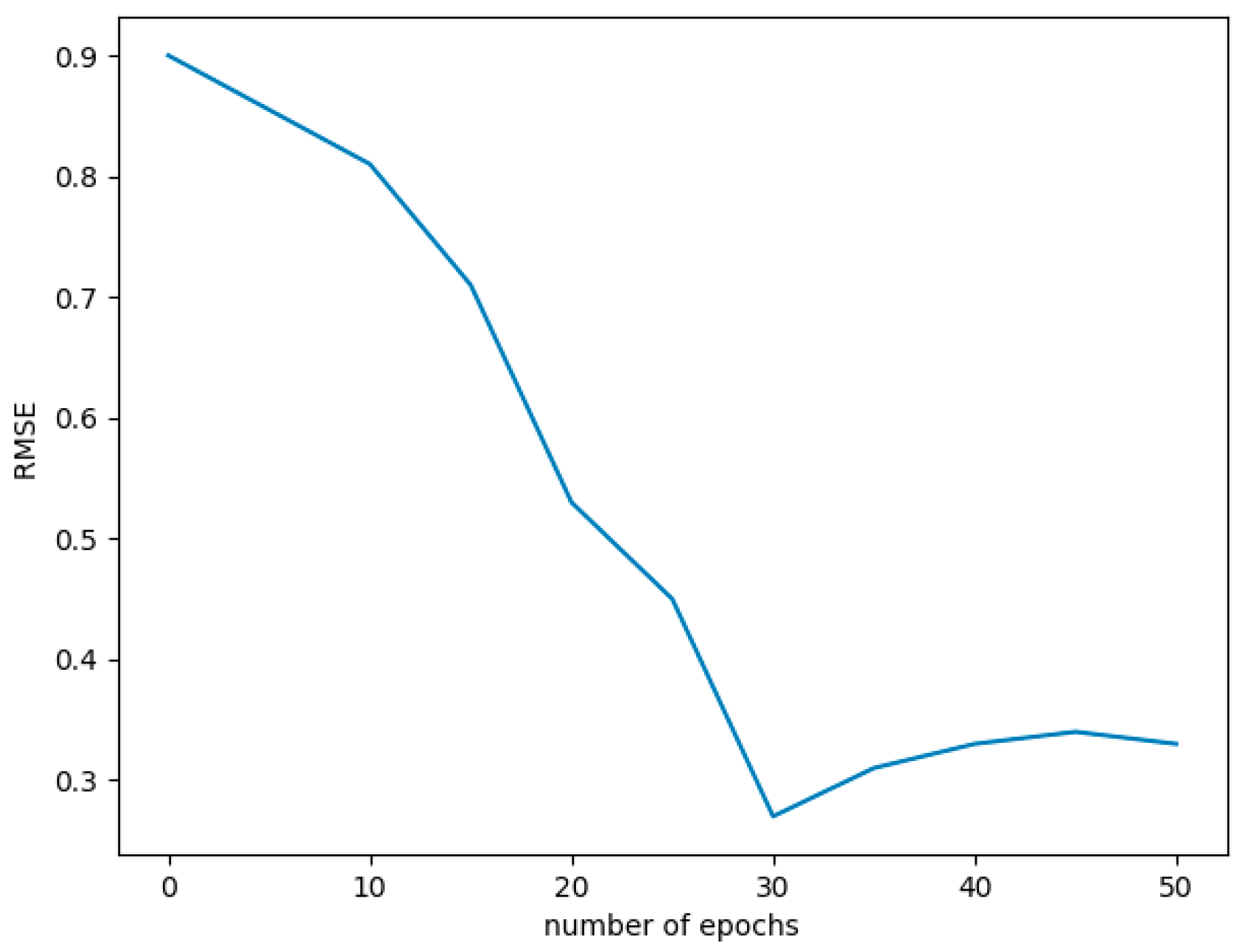
In this section, all the simulation results, comparisons and validation of the recommended prediction model are discussed. RMSE is the standard deviation of the prediction errors (residuals). As a performance assessment for the reduced prediction error of the proposed methodology, RMSE is calculated. Computed RMSE is plotted against the number of epochs for Intensified LSTM model and is shown in Figure 3. It can be seen that RMSE reduces itself to a minimum of 0.25 in 30th epochs, but the network was trained further to achieve good accuracy, learning rate and loss minimization. At the 40th epoch we obtain RMSE as 0.33, and it fluctuates at around the same for further epochs.

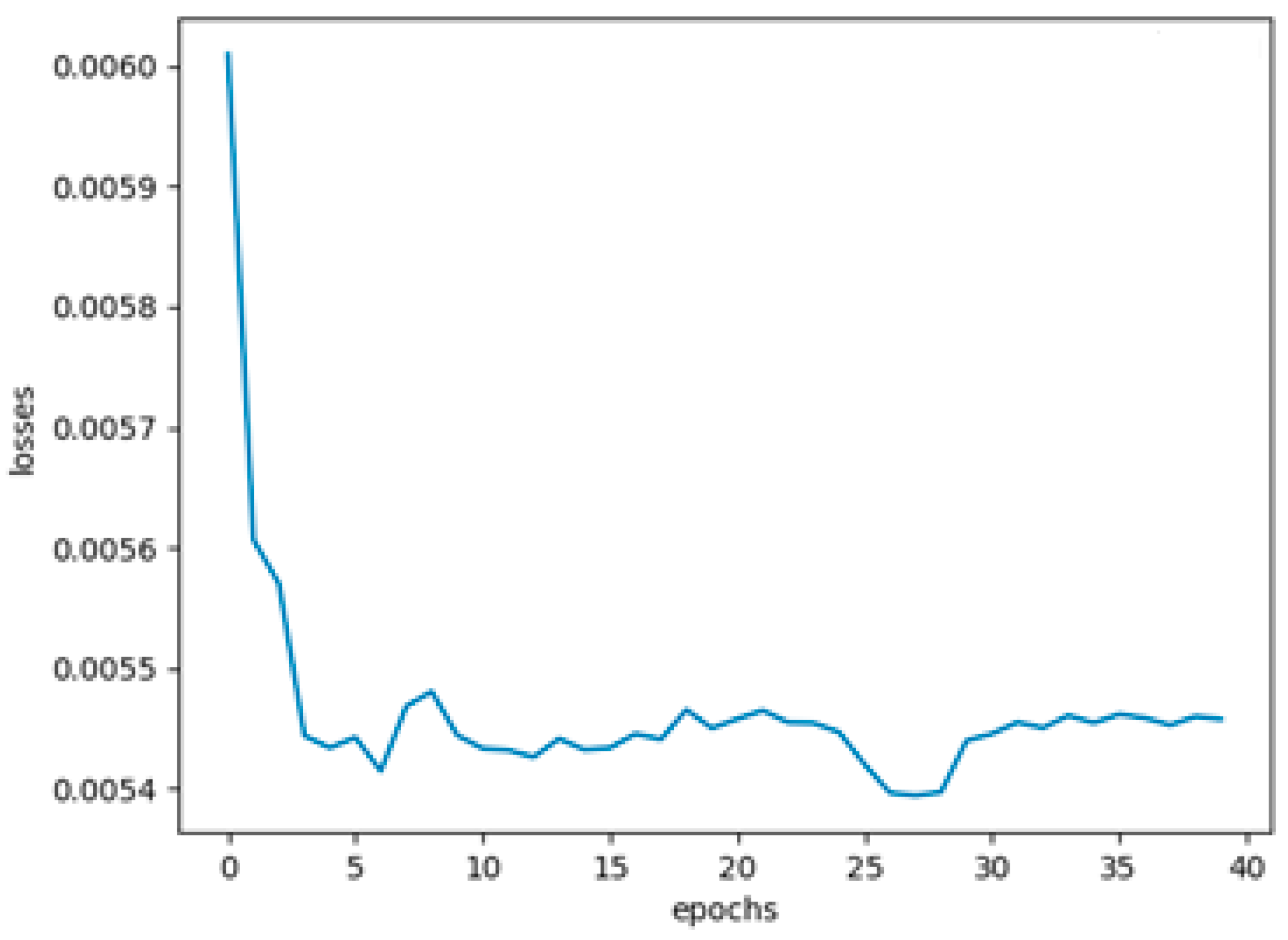
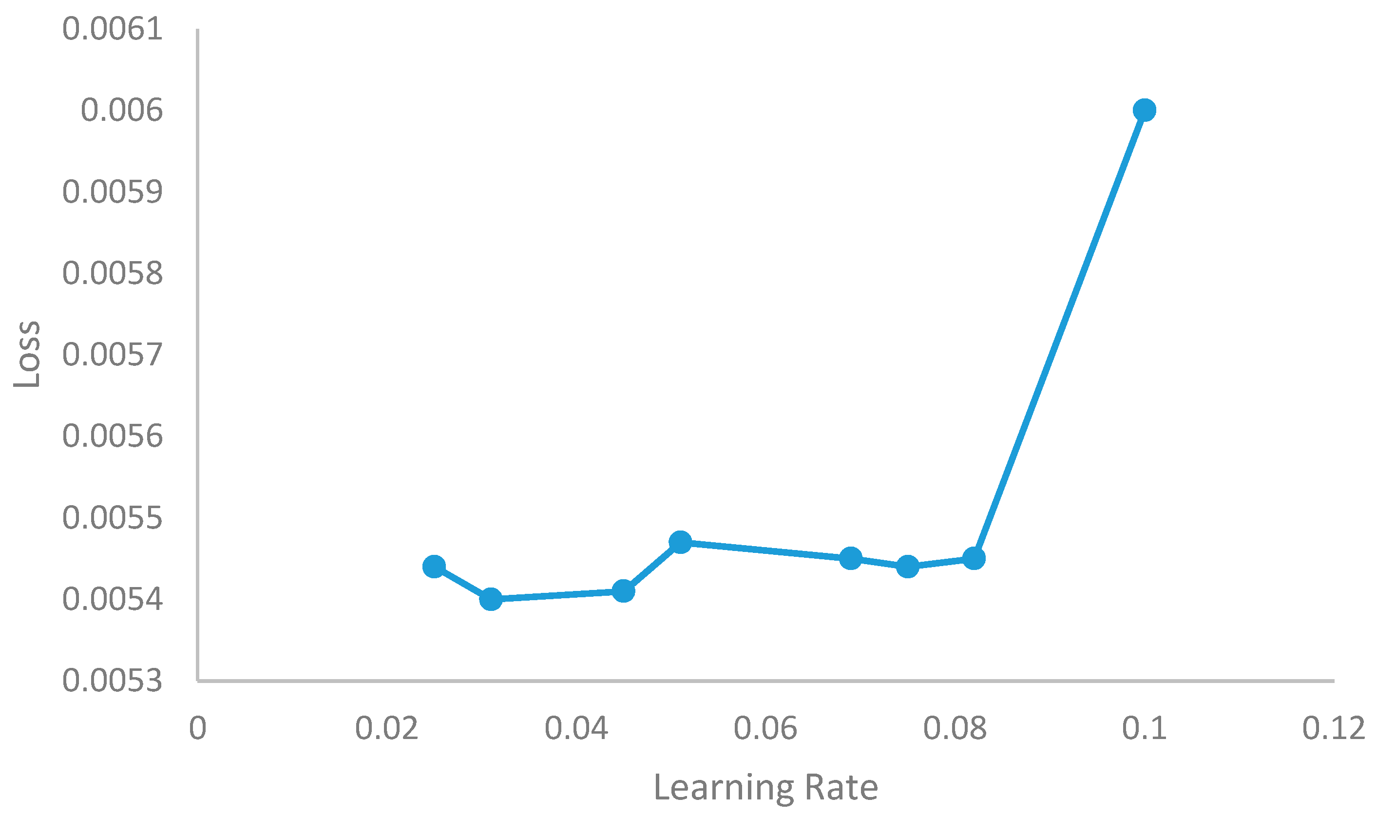
The difference between the actual rainfall attributes and predicted rainfall attributes is the error value. When error values are reduced due to back-propagation, then the deviation of predicted output with actual output is minimized, which in turn is defined as loss. Errors are reduced gradually by achieving stability, and the gradient persist through the proposed model, which leads to minimal losses. These losses are plotted against the number of epochs and are displayed in Figure 4. It can be seen that the losses are reduced drastically in the initial epochs and stay within reduced bounds in the succeeding epochs. The global minimum is found to be 0.0054 at around 27 epochs and remains within 0.0055 until the 40th epoch, which shows the stability of the proposed model.

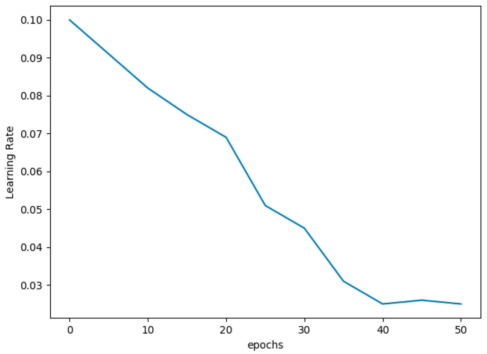
Learning rate is the hyper parameter that determines to what extent newly acquired data overrides the old ones, which means the adjustment of weight based on the loss gradient. To achieve a good learning rate, there must not be high peaks or drastic change in the graph. Therefore, the learning rate is expected to have a gradual reduction with respect to the appropriate weight modification. The proposed Intensified LSTM acquires this property with a value of 0.025 at the 40th epoch whereas the proposed model does not have significant change in learning rate for further epochs. For every epoch, the learning rate is calculated for the proposed model, and the values are plotted as a graph, as shown in Figure 5. The learning rate converges at the 40th epoch and does not get stuck with the plateau region, which proves that the proposed model self-stabilizes for the appropriate input vector in training.

The initial learning rate is fixed to 0.1 which is the value used to multiply with the weight for weight adjustment. It was expected that network loss would be minimized to certain level as the number of epochs are increased. As expected, loss subsided, and in turn, the learning rate value also diminished. An optimized level was reached at around the 30th epoch in both network loss and error, but learning rate value was around 0.04, and accuracy was around 83% at this stage. To trace out a better improvement, the network was trained further up to 40 epochs, which led to a better learning rate at 0.025, after which there was an oscillation in losses without a drastic change, which is shown in Figure 4, Figure 5 and Figure 6.

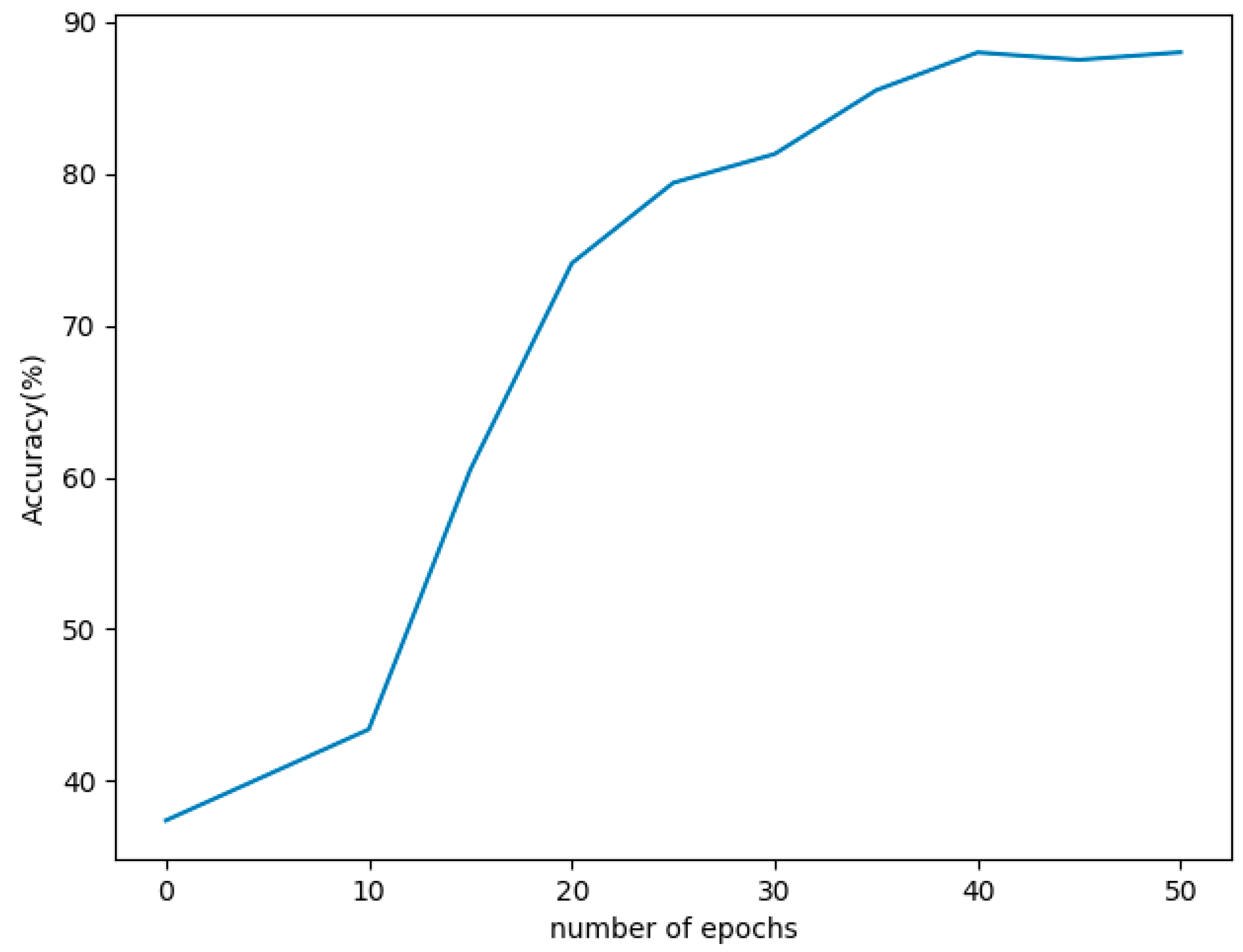
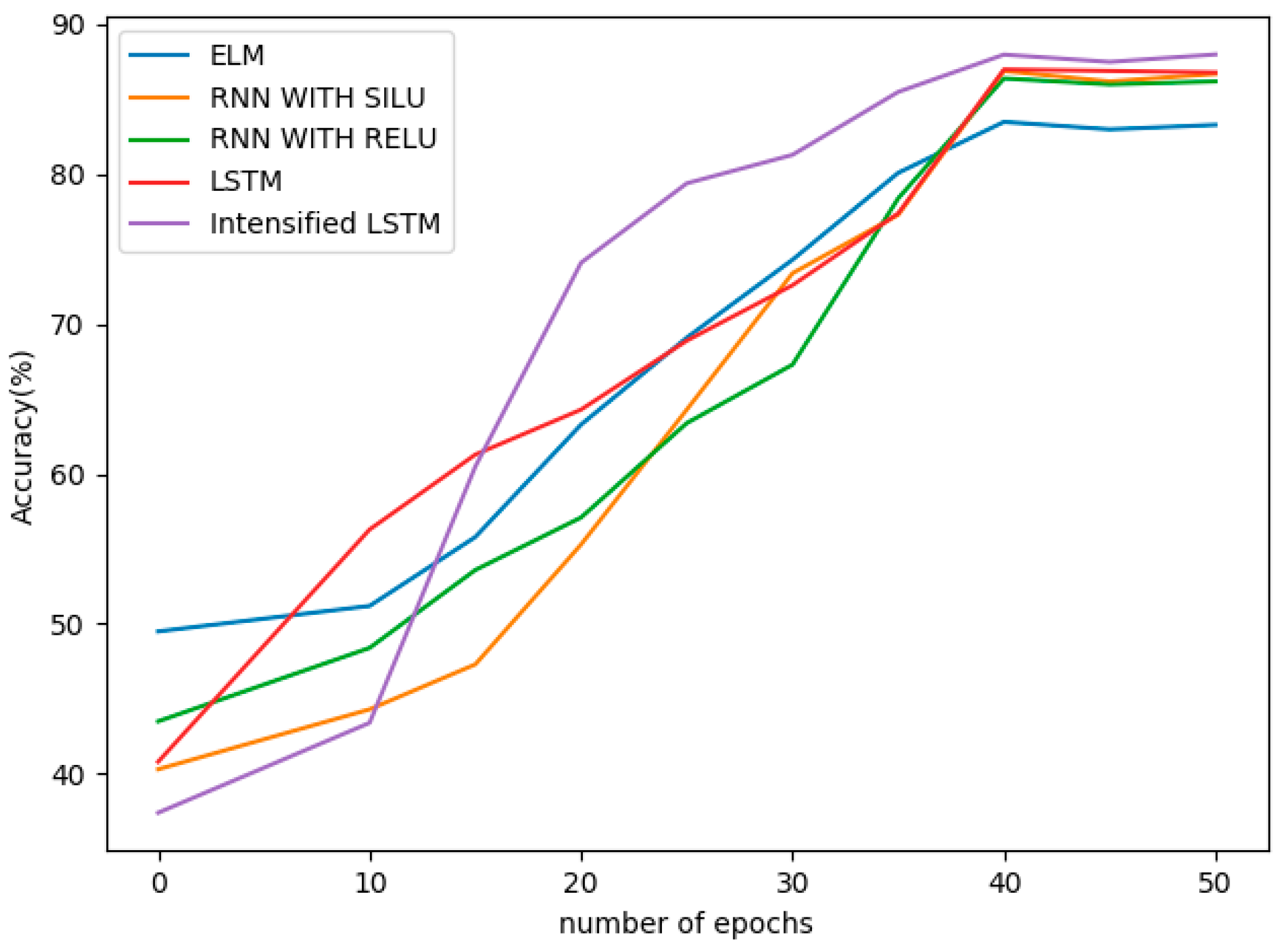
When the difference between actual value and predicted value is defined as error, accuracy can be stated as how close the predicted value is to the actual value. In such way, accuracy is calculated at every epoch and is plotted in the graph shown in Figure 7. It can be seen that accuracy increases as the number of epochs increase. Accuracy thus obtained at the 40th epoch is 87.99, almost 88%. As the graph shows, a better accuracy of 86% is obtained after the 30th epoch, where the loss and RMSE are also found to be minimal, around the same region for the Intensified LSTM with a learning rate of 0.04. The proposed model is extended for training to focus on the convergence of learning rate. As expected, the learning converges at 0.025 with increase in accuracy, and there was no significant change in accuracy as shown in the graph.

The results are validated with six other models, namely, Holt–Winters, ARIMA, ELM, RNN with Relu activation, RNN with Silu activation function and LSTM. Since Holt–Winters and ARIMA are statistical forecasting methods, the comparison is not shown with respect to parameters like epochs and losses. ELM does not include back-propagation; hence, there was no use of measurement of loss and learning rate. Performance evaluation metrics such as accuracy, RMSE, losses and learning rate values of all the seven models are in

Table 1. Performance comparison table.

Method	Epochs	Accuracy (%)	RMSE	Losses	Learning Rate
Holt–Winters	-	77.55	3.08	-	-
ARIMA	-	81.15	2.84	-	-
ELM	-	63.51	5.68	-	-
RNN with Relu	40	86.44	0.76	0.5824	0.9
RNN with Silu	40	86.91	0.76	0.5769	0.75
LSTM	40	87.01	0.35	0.1274	0.5
Intensified LSTM	40	88	0.33	0.0054	0.025

for comparison and validation of the proposed model.

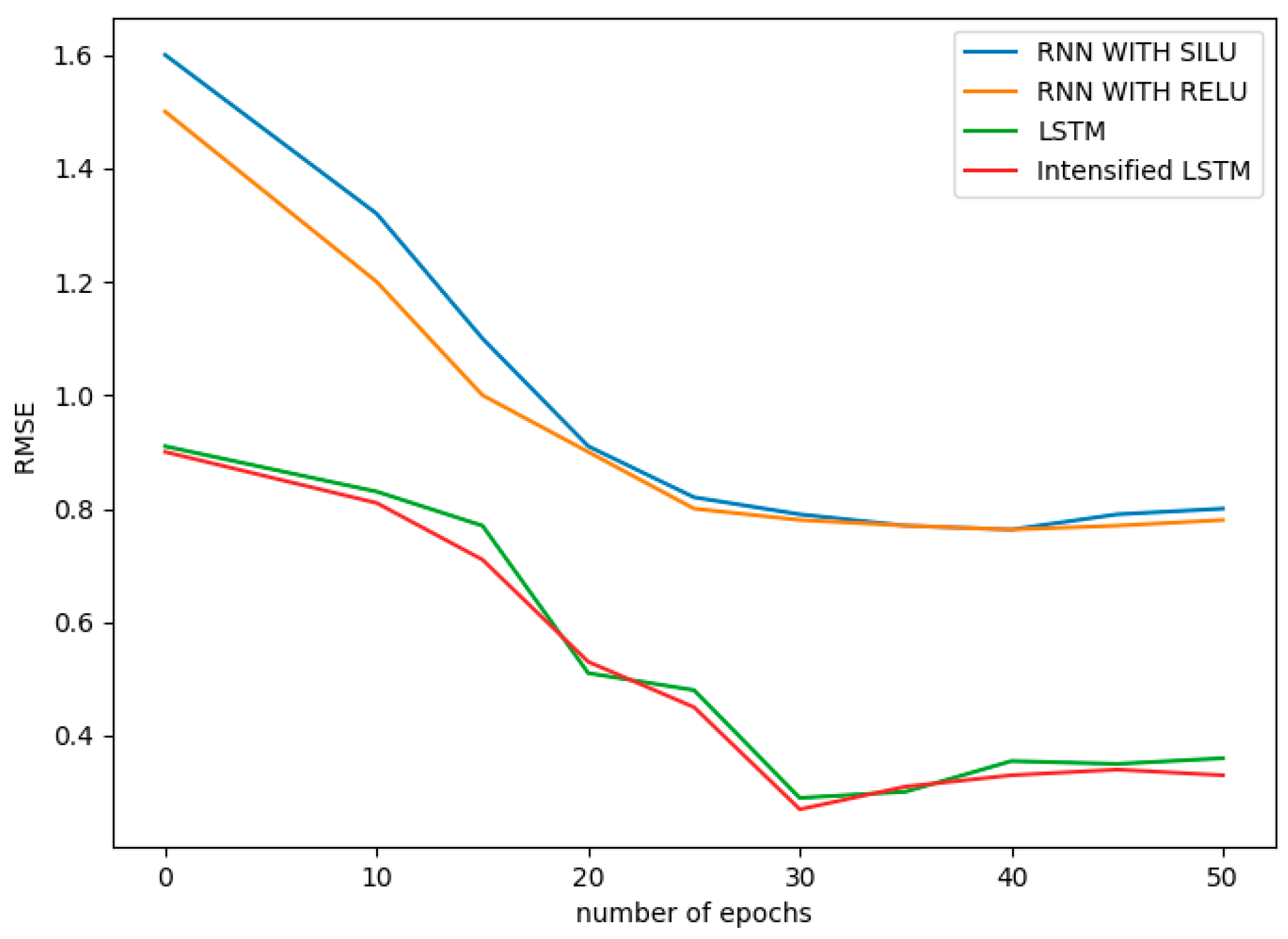
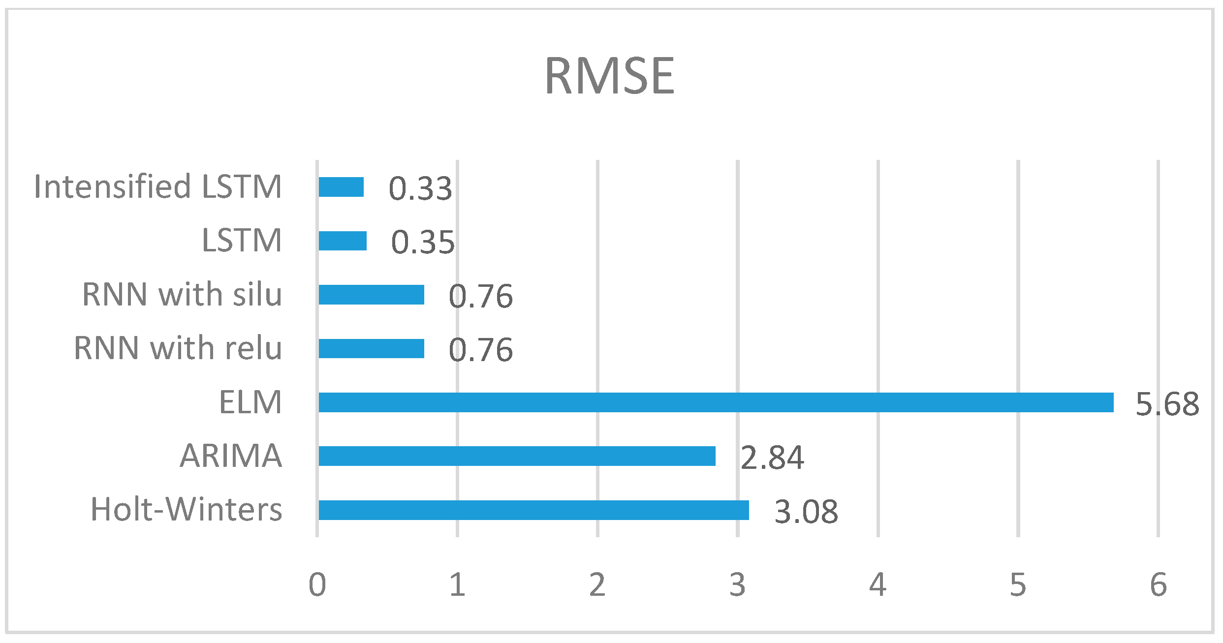
RMSE of our proposed system is compared with the aforementioned models, and the comparison is shown in Figure 8. The RMSE values obtained for the methods Holt–Winters, ARIMA, ELM, RNN with Relu, RNN with Silu and LSTM are 3.08, 2.84, 5.68, 0.7631, 0.7595, 0.35 respectively, whereas the RMSE of Intensified LSTM is 0.33. The graph infers that RMSE of LSTM based RNN models shows better results than RNN without LSTM units in the hidden layer. This is due to the long-term cell state information maintained by LSTM.

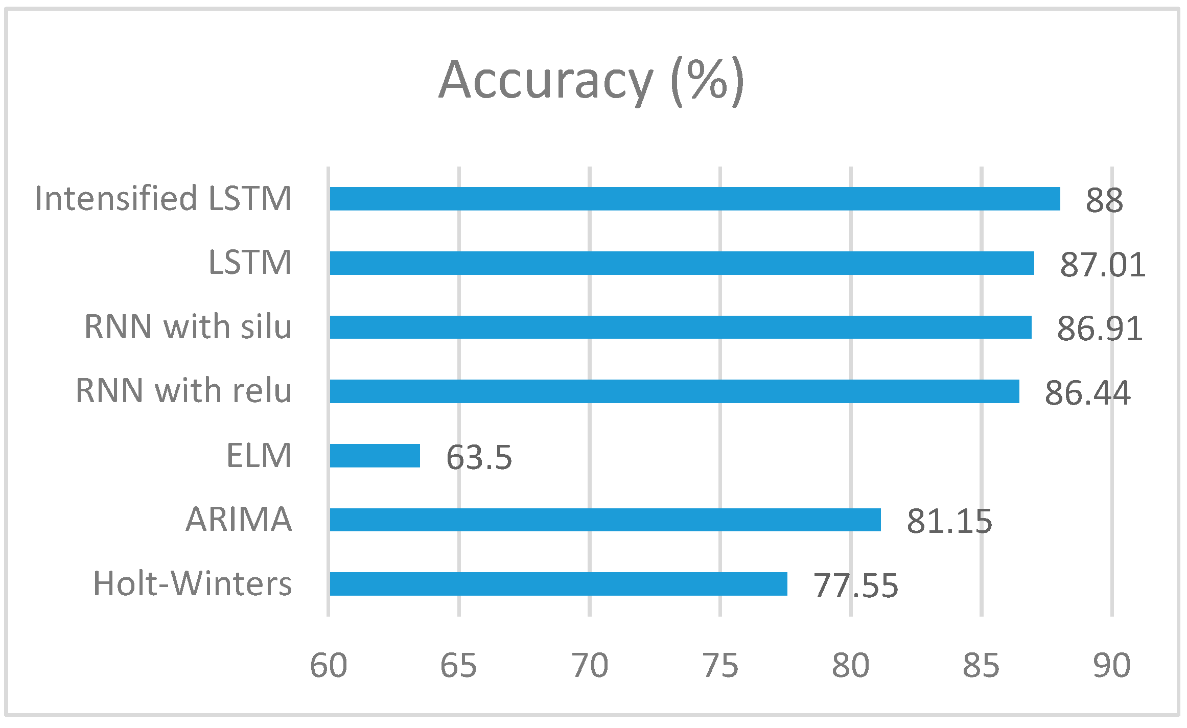
Validation of our proposed system is further done with respect to accuracy. Accuracy of these models was compared with the Intensified LSTM, and it was found that the accuracy of Intensified LSTM is better than that of Holt–Winters, ARIMA, RNN, ELM and LSTM models. Figure 9 illustrates the superiority of the proposed prediction model over other prediction models. Accuracy achieved by the Intensified LSTM based rainfall prediction model is 87.99%.

The comparison of accuracies and RMSE of the predictive models, including the statistical methods, is shown in the form of a bar chart in Figure 10. This demonstrates how efficiently\rainfall is predicted by the proposed Intensified LSTM based RNN model. It can be understood that the RNN models work well for time series data compared to statistical models that cannot handle the non-linear data as efficiently as a neural network. In neural networks, method like Extreme Learning Machine which is faster in computation are less accurate due to the absence of recurrence through which the previous state information is not fed into the network for prediction. Our proposed method is an efficient prediction model of rainfall that can aid the agricultural sector and significantly contribute to the economy of the nation.

When the RMSE of all the methods is compared, the statistical methods compete with the LSTM based model since the Holt–Winters method uses smoothing parameters like level, trend and seasonal components to control the data pattern, and ARIMA converts the non-stationary data to stationary data before prediction. ELM gives very high RMSE due to the absence of weight tuning. RNN with Relu and Silu activation function almost performs the same, whereas using LSTM units in RNN reduces the error considerably compared to RNN without LSTM. RMSE comparison of all the methods used in this research work is shown in Figure 11.

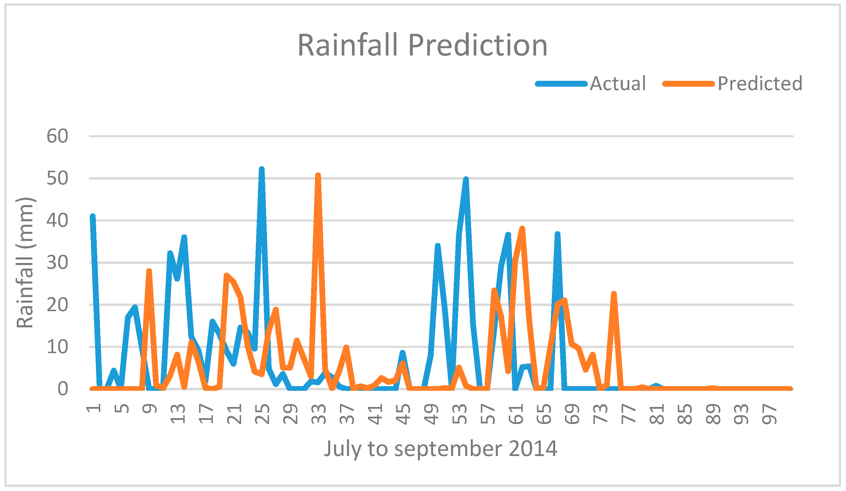
The actual rainfall and predicted rainfall are plotted and shown in Figure 12. The predicted rainfall values in mm are plotted for 97 days from July to September 2014, having considered 34 years of previous data as training inputs. Holding such a huge dataset is possible only because of the use of LSTM unit in RNN network. This plot is compared with the plot of actual rainfall data of the same year to assess the performance of the model to track the actual graph. It can be seen that the predicted values almost match the actual values except for the peaks. The reason is some data points in the dataset may be considered as outliers, that induces so much deviation in the consecutive values. The prediction methods try to either eliminate these points or map them by analyzing whether such pattern exists already during the training phase.

5. Conclusions

People are always interested in knowing about future occurrences Data is abundant nowadays but analyzing the data and inferring the hidden facts is done to a lesser degree. Thus, data analytics and improvements in the prediction model can provide insights for better decision making regardless of applications. In this research paper, deep learning approach is carried out for rainfall prediction. Intensified LSTM based Recurrent Neural Network is constructed to predict rainfall. This approach is compared with other methods, namely, Holt–Winter, ARIMA, ELM, RNN and LSTM, in order to demonstrate the improvement of rainfall prediction in the proposed approach. For attaining good accuracy, it is necessary to consider previous datasets. Since the proposed Intensified LSTM network could hold large data in its memory and could avoid the vanishing gradient, it appears to show better accuracy in prediction. Although the improvement in accuracy is little in the proposed Intensified LSTM compared to existing LSTM model based RNN, the proposed prediction model preserves that accuracy for further epochs, while exhibiting reduced loss, RMSE and learning rate. Any neural network which pulls off an adequate learning rate with depletion in loss within fewer epochs is deemed sustain itself for any test data applicable in the future without much oscillation in performance metrics such as accuracy, error, etc. Achieving better results in fewer epochs reduces the running time that helps in processing and analyzing big data which possess high volumes of data. The proposed model achieves the above mentioned performance.

In future work, this predicted dataset of rainfall can help in the hydrological identification of drought, which is a major concern in agriculture. Type of soil may be an important consideration to sow a crop, but whatever may be the type of soil, rainfall is the main source for better vegetation. Therefore, our research work will be continued by analyzing the positive and negative effects based on the results of rainfall prediction, which is helpful to perform prescriptive analytics.