Abstract
In the near future, there will be several new instruments measuring atmospheric composition from geostationary orbit over North America, East Asia, and Europe. This constellation of satellites will provide high resolution, time resolved measurements of trace gases and aerosols for monitoring air quality and tracking pollution sources. This paper describes a detailed, fast, and accurate (less than 1.0% uncertainty) method for calculating synthetic top of the atmosphere (TOA) radiances from a global simulation with a mesoscale free running model, the GEOS-5 Nature Run, for remote sensing instruments in geostationary orbit that measure in the ultraviolet-visible spectral range (UV-Vis). Generating these synthetic observations is the first step of an Observing System Simulation Experiment (OSSE), a framework for evaluating the impact of a new observation or algorithm. This paper provides details of the model sampling, aerosol and cloud optical properties, surface reflectance modeling, Rayleigh scattering calculations, and a discussion of the uncertainties of the simulated TOA radiance. An application for the simulated TOA radiance observations is demonstrated in the manuscript. Simulated TEMPO (Tropospheric Emissions: Monitoring of Pollution) and GOES-R (Geostationary Operational Environmental Satellites) observations were used to show how observations from the two instruments could be combined to facilitate aerosol type discrimination. The results demonstrate the viability of a detailed instrument simulator for radiance measurements in the UV-Vis that is capable of accurately simulating high resolution, time-resolved measurements with reasonable computational efficiency.
1. Introduction
Within the next five years, several new instruments will be launched into geostationary orbit with the objective of monitoring air quality. This geostationary constellation will be comprised of TEMPO (Tropospheric Emissions: Monitoring of Pollution) over North America [1], Sentinal-4 over Europe [2], and GEMS (Geostationary Environment Monitoring Spectrometer) over East Asia [3], and will provide an unprecedented level of high-resolution (both spatially and temporally) atmospheric composition data. The three spaceborne platforms will measure ozone (O), nitrogen dioxide (NO), sulfur dioxide (SO), formaldehyde (HCHO), and aerosols from backscattered radiation in the ultraviolet-visible spectral range (UV-Vis). The large-scale, time-resolved measurements of these pollutants provided by the geostationary constellation are important for managing air quality, and understanding how human activity impacts local, regional, and global distributions of pollution, as well as global climate.
Aerosols are one of the most important forcing agents in the climate system. They can be transported around the globe [4], and interact with weather systems [5], scatter and absorb radiation [6,7,8], and modify cloud properties [9,10]. Routine measurements of various aerosol parameters, such as aerosol optical depth (AOD), absorbing aerosol optical depth (AAOD), aerosol index (AI), and single scattering albedo (SSA), are currently available from several sensors in low earth orbit (LEO). These sensors include the twin MODIS (Moderate Resolution Imaging Spectroradiometer) instruments (on-board Terra and Aqua), MISR (Multi-angle Imaging SpectroRadiometer), OMI (Ozone Monitoring Instrument), and POLDER (Polarization and Directionality of the Earth Reflectances) (see Table 1 in [11]). In addition, CALIOP, a spaceborne LiDAR, measures the vertical distribution of aerosol backscattering.
Instruments in LEO provide one or two measurements per day, but as aerosol parameters cannot be retrieved under cloudy conditions there can be a large time interval between valid observations. This limits the capability of LEO measurements to track the evolution of aerosol distributions, while a geostationary constellation can provide a continuous view of the areas below the satellites. TEMPO, GEMS, and SENTINEL-4 will provide measurements at a temporal resolution of approximately one hour, enhancing the probability of observing cloud-free scenes.
It is expected that the baseline aerosol products for the geostationary constellation, AOD and AI, will be based on the heritage of the OMI and TOMS (Total Ozone Mapping Spectrometer) AOD retrieval algorithms that use reflectance measurements in the UV. However, numerical studies have shown that including coincident measurements from geostationary weather satellites, such as the Geostationary Operational Environmental Satellite-R Series (GOES-R) operated by the U.S. National Oceanic and Atmospheric Administration (NOAA), at complementary wavelengths and viewing geometry can reduce the uncertainty in retrieved AOD as well as enhance the retrieval of fine-mode aerosol fraction [11]. Moreover, higher resolution observations from weather satellites can also improve the geostationary AOD retrieval by providing sub-pixel cloud information.
Estimating the usefulness and key characteristics of these planned aerosol products is essential for developing applications for these data. This type of evaluation is referred to as an Observing System Simulation Experiment (OSSE). OSSEs are performed using datasets of synthetic observations developed from a high resolution earth system simulation. The synthetic observations should sample the earth system simulation in such a way as to mimic the observation capabilities of the instrument, including its’ viewing geometry and spatial, temporal, and spectral resolution. After an algorithm is applied to the synthetic data, one can gauge the performance of the algorithm by comparing the algorithm results to the initial earth system simulation from which the synthetic data was created (i.e., the OSSE “truth”).
In order to generate synthetic observations globally over a realistic dynamic range, a 2-year high-resolution mesoscale free-running atmospheric simulation, the Goddard Earth Observing System version 5 (GEOS-5) Nature Run (G5NR) [12], was completed. The G5NR has been validated against nature [13], and provides a realistic representation of global aerosol concentrations and climate. As the GEOS-5 Nature Run includes aerosols, we are able to extend OSSEs beyond traditional weather forecasting applications.
Several studies have explored the ability of geostationary observations to better constrain spatial and temporal variations of CO and O [14,15,16,17], and have shown that geostationary satellites have the potential to address the limitations of the current observing system. In comparison, only Timmermans et al. [18] has presented an OSSE for aerosols. They found that hourly geostationary AOD observations over Europe improved the ground level particulate matter analysis and forecast.
The goal of this paper is to describe the aerosol nature run, G5NR, and its’ application to forward model calculations for generating synthetic observations for aerosol OSSEs. These synthetic data will be used to test AOD retrieval algorithms over realistic conditions, and to understand the impact of the geostationary constellation on global aerosol data assimilation and forecast products. Aerosol OSSEs require detailed radiative transfer modeling of top of the atmosphere (TOA) reflectance to generate synthetic observations rather than averaging kernel regression methods, such as those used for CO and O OSSEs, because aerosol distributions have higher spatial variability, and operational AOD retrievals rely on multi-step retrieval approaches (that can vary depending on the type of aerosol detected) rather than formal optimal estimation to retrieve AOD. In Section 2, we describe the TEMPO, GEMS, and SENTINEL-4 instruments, as well as the G5NR aerosol simulation. This is followed by a description of the methodology used to generate synthetic TOA reflectance with VLIDORT (Vector Linearized Discrete Ordinate Radiative Transfer), the forward radiative transfer model. In Section 3, we present examples of simulated observations for TEMPO, GEMS, and SENTINEL-4 and describe an estimate of their uncertainty in Appendix A. Finally, Section 4 contains a summary of the work and future perspectives.
2. Methodology and Data
2.1. Characteristics of TEMPO, GEMS, and SENTINEL-4
Figure 1 shows the expected spatial resolution for TEMPO, GEMS, and SENTINEL-4 imagery, which was determined according to a geostationary projection on the globe from their respective longitudes, listed in Table 1. The table also contains the instruments’ fields of regard and spectral ranges. Each instrument observes its’ field of regard by scanning from east to west over the course of an hour for TEMPO and SENTINEL-4, and 30 min for GEMS, which will take observations for 30 min every hour. All of the instruments will nominally cover the 300–500 nm spectral range, but SENTINEL-4 will also measure 750–775 nm to gain additional information about cloud heights from the oxygen-A band.
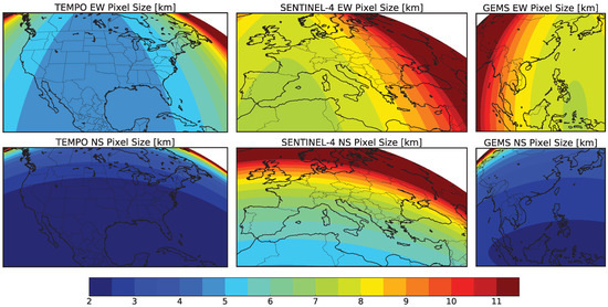
Figure 1.
Spatial resolution of TEMPO, SENTINEL-4, and GEMS. Pixel sizes were determined according to a geostationary projection on the globe from the satellites’ respective longitudes.

Table 1.
Instrument specifications for the geostationary constellation.
2.2. GEOS-5 Nature Run Aerosol Simulation
The GEOS-5 Nature Run (G5NR) is a 2-year (May 2005–May 2007) global 7 km non-hydrostatic mesoscale simulation based on the Ganymed version of GEOS-5, the NASA GMAO Earth system model. The Goddard Chemistry, Aerosol, Radiation, and Transport model (GOCART, [19]) was run online with coupling to the GEOS-5 radiation code [20], and handled the sources, sinks, and chemistry of dust, sulfate, sea salt, black carbon (BC), and organic carbon (OC) aerosols. The model tracked the total mass of sulfate, two modes (hydrophobic and hydrophilic) of organic and black carbon aerosol, and the particle size distributions of dust and sea salt resolved across five non-interacting size bins for each. The G5NR simulation was driven by the following prescribed parameters: (1) sea surface temperature and sea-ice, (2) daily sources of volcanic and biomass burning aerosols and trace gases, (3) high-resolution anthropogenic aerosol and trace gas emissions, (4) sinks of aerosols and trace gases, and (5) biogenic sources and sinks of CO.
Besides a full meteorological description of the atmosphere, the G5NR outputs contain vertical profiles (72 layers from the surface to 0.01 hPa) of concentrations of the 15 aerosol tracers, as well as O, CO, and CO at 30 min time intervals. As the aerosol mass mixing ratios were initialized at zero at the start of the G5NR time period, the first 6 months of the simulation were taken as spin-up in order for aerosol mass mixing ratios to reach equilibrium in the stratosphere. Figure 2 shows an example of the simulated instantaneous concentrations of sea salt, black and organic carbon, dust, and sulfate, and illustrates the high spatial resolution of the G5NR.
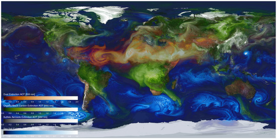
Figure 2.
The 7 km G5NR aerosol simulation for 27 July 2006 at 12 Z. Blue shading corresponds to sea salt concentration, green shading corresponds to black and organic carbon concentrations, red-orange shading corresponds to dust, and white shading corresponds to sulfate.
2.2.1. Aerosol Sources and Sinks
The following sources of aerosols were included in the model: (1) wind-speed dependent emissions of dust and sea-salt (for details see [21]), (2) anthropogenic emissions of sulfate and carbonaceous aerosol from fossil fuel combustion, biomass burning, and biofuel consumption (described below), and (3) biogenic emissions of organic carbon (for details see [21]). Oxidation of di-methyl sulfide (DMS) and SO, which had anthropogenic and volcanic sources, was an additional chemical production source for sulfate (SO). The aerosol sinks were dry deposition, wet removal, and convective scavenging. Aerosol hygroscopic growth was considered in computations of particle fall velocity and deposition velocity.
Sulfate emissions from fossil fuel combustion were taken from the Emissions Database for Global Atmospheric Research v4.2 (EDGAR; [22]), which are provided annually at 0.1° resolution. For organic and black carbon fossil fuel and biofuel aerosol emissions, which are not included in EDGAR v4.2, a hybrid database was developed using 0.1° resolution EDGAR-HTAP emissions [23] and 1° resolution emissions from the Aerosol Comparisons between Observations and Models (AeroCom) [24] Phase II project. EDGAR-HTAP emission totals for 2005 over 1° areas were adjusted to match yearly AeroCom 1° emissions estimates for 2005–2007. The relative spatial distribution of 0.1° resolution EDGAR-HTAP emissions within in each 1° area was retained. Thus, the resulting emissions database draws global total emissions and inter-annual variability from AeroCom, while using EDGAR-HTAP to achieve a high spatial resolution.
SO and SO emissions from ships were derived in the same manner from EDGAR-HTAP and AeroCom emissions. Non-shipping emissions of SO were taken directly from EDGAR v4.1 estimates for 2005 because of errors in AeroCom emissions. DMS emissions from marine algae were based on the monthly varying climatology described in [25].
Biomass burning emissions of OC, BC, and SO were obtained from the Quick Fire Emissions Dataset (QFED) version 2.4-r6 [26]. QFED is based on the fire radiative power (top-down) approach and includes the cloud correction method used in the Global Fire Assimilation System (GFAS) [27]. However, it also employs a more sophisticated treatment of emissions from non-observed land areas. Fire locations and fire radiative power were obtained from the Moderate Resolution Imaging Spectroradiometer (MODIS) Level 2 fire products and the MODIS geolocation products. Daily mean fire emissions were created from the MODIS Level 2 fire products re-gridded to 0.1° × 0.1° horizontal resolution. In the model, a diurnal cycle in fire emissions that is more prominent in the tropics and gradually weakens at higher latitudes in the North hemisphere’s temperate zone was imposed on the daily mean emission values.
The major chemical production and loss pathways of SO, SO, and CO were accounted for by the GOCART tropospheric chemical mechanism, which includes gas-phase and aqueous-phase reactions. The chemical mechanism was driven by prescribed monthly mean concentrations of several key trace gases and radicals, namely methane (CH), hydroxyl radical (OH), nitrate radical (NO) and hydrogen peroxide (HO). The prescribed fields were generated from a simulation of the NASA Global Modeling Initiative (GMI) model driven by assimilated meteorological data from MERRA (Modern-Era Retrospective Analysis for Research and Applications) [28,29,30]. A diurnal variation of OH concentration was computed by scaling the monthly mean fields by the cosine of the solar zenith angle. A diurnal variation of NO was imposed by assuming zero concentration in daylight and the monthly mean concentration at night. Because HO is the limiting agent in the aqueous phase formation of SO, its’ concentration was reset every three hours to the monthly mean values.
2.2.2. Evaluation of G5NR Aerosols
Aerosol concentrations in the G5NR simulation were evaluated with the following datasets [13]: (1) global concentrations from the NASA/GMAO MERRA Aerosol Reanalysis (MERRAero) [31], (2) statistics from the AeroCom Phase I models [32], and (3) CALIOP aerosol attenuated backscatter vertical profiles [33]. The evaluation was meant to assess the overall realism of the simulated aerosols, and mainly focused on broad performance metrics of the simulation such as aerosol residence times, and the spatial and temporal distributions of aerosol composition and AOD. As the G5NR is a free running simulation, differences are to be expected between the distributions of observed and simulated atmospheric composition due to meteorological variability.
G5NR aerosol residence times, and wet and dry removal rates are listed in Table 2. The residence time is defined as the global aerosol total column mass divided by the removal rate (See Section 6 in [32]). Also included in the table are the AeroCom multi-model mean parameters and their standard deviations reported in Textor et al. [32]. The residence times of sea salt, dust, and black carbon agree well with the AeroCom multi-model means. The residence time of organic carbon in G5NR is roughly one day less than the AeroCom mean, but lies well within one standard deviation of the mean. However, the residence time of sulfate aerosol is significantly (36%) lower than what is reported by the AeroCom models. The shorter sulfate residence time in G5NR is due to the relatively high wet removal rate of the simulation of 0.34 days.
Table 2.
Residence and removal rates of aerosols in G5NR. The residence times in parenthesis are multi-model means and standard deviations from the AeroCom project reported in [32].
The 2006 seasonal mean 550 nm AOD (AOD) is shown in Figure 3 from the MERRAero Reanalysis and G5NR. The MERRAero aerosol reanalysis includes assimilation of AOD observations from the MODIS sensor on both Terra and Aqua, and provides a climatology of the aerosol spatio-temporal distribution. Overall, the seasonal and spatial patterns in G5NR are very similar to MERRAero. Patterns of aerosol enhancements agree well with the major sources and transport routes of aerosols. However, over Africa and along the westward transport route of Saharan dust, G5NR AOD is systematically higher than MERRAero. Likewise, G5NR AOD is higher than MERRAero in the regions affected by dust that originate from sources in the Middle East.
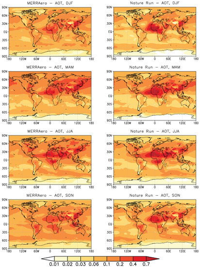
Figure 3.
2006 seasonal mean 550 nm AOD from the MERRAero aerosol reanalysis (left column) and the G5NR (right column). Time-averaged values for DJF, MAM, JJA, and SON are organized from top to bottom.
Figure 4 shows the monthly time series of global mean AOD for MERRAero and G5NR. The G5NR temporal variability and the magnitude of the global mean AOD are similar to the aerosol climatology, which is expected given the similarities in the primary emissions. However, there are significant differences between G5NR and MERRAero in speciated global mean AOD. Underestimated carbon and sulfate were compensated by overestimated dust. This indicates that the wind driven dust emissions and resolution dependent biomass burning emissions should be re-tuned for the mesoscale resolution of G5NR.
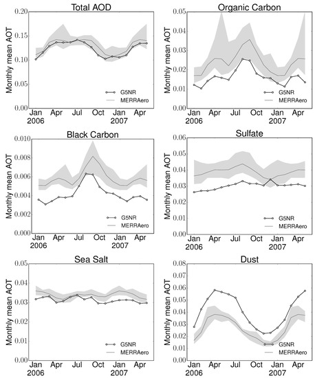
Figure 4.
Time series of global monthly mean 550 nm AOD. Results from the G5NR simulation are in black. The monthly mean climatology from the MERRAero reanalysis is shown in gray; the shaded area encloses the minimum and maximum monthly means from the 14-year time series (2002–2016), while the gray line represents the mean.
The observed similarities between G5NR and MERRAero in the temporal patterns of the speciated 550 nm AODs enables us to derive global scaling factors for each of the aerosol species. The global scaling factors were computed from linear regression of the G5NR and MERRAero AOD while constraining the intercept to zero, and are listed in Table 3. On a global scale, BC, OC, sulfate, and sea salt AOD should be increased by the factors 1.43, 1.36, 1.30, and 1.08, respectively, to match MERRAaero. Meanwhile, dust AOD should be decreased by a factor of 0.67. For certain applications of the G5NR data, such as sampling studies to quantify the likelihood that an orbit will encounter certain aerosol mixtures, it is recommended that users apply these scaling factors to adjust the speciated AOD.
Table 3.
Global 550 nm AOD Scaling Factors.
G5NR simulated aerosol vertical distributions were compared to cloud-cleared CALIOP Level 1.5 aerosol attenuated backscatter vertical profile data [34] in Figure 5 and Figure 6. This is a spatially averaged cloud cleared product suitable for comparison to aerosol transport models. We focused our analysis on two different regions during the month of July, when large plumes of dust and biomass burning aerosol are found off the west coast of Africa. The dust dominated region included the Sahara and the North Atlantic Ocean (60° W – 20° E, 0° N – 30° N), and the biomass burning region covered southern Africa (10° W – 30° E, 0° S – 30° S).
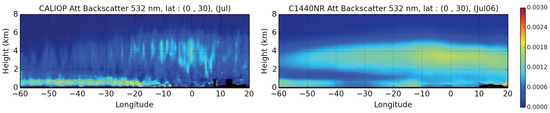
Figure 5.
Vertical profiles of aerosol attenuated backscatter coefficient at 532 nm over the African dust region (60° W – 20° E, 0° N – 30° N). On the left are time-averaged retrievals from CALIOP for July 2011. On the right is the G5NR simulation July 2006.
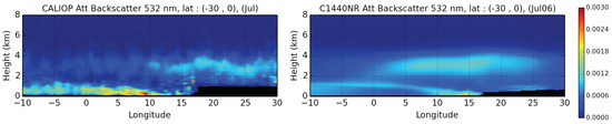
Figure 6.
Same as Figure 5 but for the southern Africa biomass burning region (10° W – 30° E, 0° S – 30° S).
Figure 5 shows the monthly mean comparison over the Saharan dust region between CALIOP and G5NR aerosol attenuated backscatter at 532 nm. The monthly mean for the model was calculated with data for July 2006, while for CALIOP observations from July 2011 were used. Only one observation year was considered due to the limited availability of Level 1.5 data at the time of this analysis. This comparison should be viewed as a qualitative assessment of the G5NR aerosol vertical distributions because the Nature Run has not been sampled along the CALIPSO orbit track. Furthermore, as G5NR is a free running simulation, it does not represent a prediction for a specific observation year. Nevertheless, the observed and simulated aerosol backscatter vertical profiles have similar vertical structures, with a dust plume that extends to roughly 6 km over the Sahara and descends westward to the Caribbean over a shallow marine aerosol layer. However, the magnitude of the attenuated backscatter of the elevated dust plume in G5NR is higher than what is observed by CALIOP. This further indicates that dust emissions in G5NR over this region are likely overestimated. However, these differences could also be due to interannual variability in the spatial distribution of elevated dust in the North Atlantic.
Figure 6 shows the comparison between CALIOP and G5NR over the southern Africa biomass burning region. The simulation and observations again have a similar vertical structure. In this case, the smoke plume extends up to 4 km above a marine aerosol layer that can reach an altitude of ∼1.5 km for both G5NR and CALIOP. While the magnitude of the simulated aerosol backscatter for the smoke plume is in the range of the CALIOP estimates, the simulated backscatter for the marine aerosol layer tends to be weaker than what is observed.
2.3. Surface Reflectance Models
For each satellite domain and observation wavelength, the highest resolution available surface reflectance dataset was used. For simplicity, this first version of the simulator we considered only land surfaces, while future versions will consider water leaving radiance. Over land, for visible and near infrared channels, we used the Ross-Thick Li-Sparse (RTLS) model [35] to represent the variations in surface reflectance as a function of measurement and illumination angles (i.e., the bidirectional reflectance distribution (BRD)). In this model the BRD is calculated by a linear combination of three semi-empirical kernel functions:
where , , are the isotropic (Lambertian), geometric [36], and volumetric [37] kernel functions, and , , and are their respective amplitudes (or weights). The kernels represent different modes of surface scattering. The kernel weights are derived from MODIS observations, such that when the three kernels are scaled by their weights the modeled surface reflectance matches the observations.
Equations (2)–(4) show the formulations for the three kernels based on the solar zenith (), viewing zenith (), and relative azimuth angles, which are defined according to the photon travel direction, such that is the forward scattering direction ( and are the viewing and solar azimuth angles, respectively). In Equation (3), for the Li-Sparse (geometric) kernel, h, b, and r represent the height of the crown center, the vertical crown radius, and horizontal crown radius, respectively. The crown relative height () was set to 2, and the crown shape parameter () was set to 1 (consistent with the MODIS retrievals).
The MCD43D product provides daily kernel weights [35] on a 30 arc second grid. The dataset was gap-filled with a seasonal climatology. Eight-day RTLS kernel weights at 1 km resolution from the MAIAC (Multi-Angle Implementation of Atmospheric Correction) algorithm [38,39] (only available over North America at the time of this work) were used for the TEMPO domain.
When using the RTLS model to represent surface reflectance, VLIDORT treats surface reflectance as “scalar”, i.e., reflectance is only applied to the total intensity (I) term of the Stokes vector; only the (1,1) component of the BRD matrix is non-zero.
Figure 7 shows an example of the change in surface reflectance at 670 nm as would be observed by TEMPO due to the changing sun-sensor geometry on a typical day, and indicates the importance of using a rigorous radiative transfer model with a non-Lambertian surface.
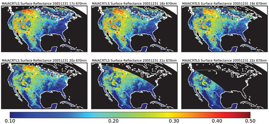
Figure 7.
Simulated surface reflectance according to the MAIAC BRDF retrieval at 670 nm for the TEMPO sun-sensor geometry at 17–22 Z on 31 December 2005. Changes in the surface reflectance throughout the day are due to the bidirectional nature of the surface reflectivity.
For the 354 and 388 nm channels, which fall outside of the range of the MODIS observations, we used a global 0.25° monthly climatology of Lambertian surface reflectance that was based on TOMS observations (Hiren Jethva, personal communication) interpolated to the satellite grids. Figure 8 shows the December Lambertian surface reflectance from the climatology dataset on the three instrument domains.
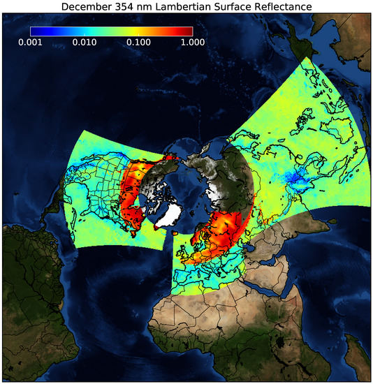
Figure 8.
Lambertian equivalent reflectance mapped to the TEMPO grid from a 0.25° monthly climatology based on TOMS observations.
2.4. TOA Radiance Simulations
Our approach to simulating TOA radiance for TEMPO, GEMS, and SENTINEL-4 is to first simulate radiance at scales smaller than the satellite resolution, and then aggregate the sub-pixels to the satellite resolution using the independent pixel approximation. This approach allows us to simulate realistic sub-grid scale variability of surface and cloud reflectance. The higher resolution radiance dataset also allows us to test different approaches to combining simultaneous measurements from the relatively coarse resolution air quality satellites with higher resolution weather satellites, such as GOES-R. The nominal sub-pixel resolution in our simulations is 1 km, corresponding to, for example, 8 sub-pixels for every one 2 km by 4 km TEMPO pixel.
To achieve this high resolution radiance simulation we use high resolution surface reflectance datasets (when available), and statistically downscale the G5NR simulated moisture fields following the approach in Norris et al. [40], which derives cloud liquid water path, cloud ice water path, and relative humidity for each sub-pixel. Aerosol dry mass mixing ratios in the sub-pixels are derived from interpolating the G5NR model outputs to the coarse TEMPO, GEMS, and SENTINEL-4 grids, which have comparable resolutions. Thus, because we lack a reliable method to downscale the aerosol concentration further, the aerosol dry mass mixing ratios within the coarse satellite pixel is constant. However, the downscaled 1 km relative humidity data is used to determine the aerosol hygroscopic growth, allowing for sub-grid scale variability in aerosol optical properties.
2.4.1. Generating Sub-Grid Cloud Pixels
The 1 km cloud sub-pixels were generated from the G5NR simulation using a statistical model of sub-grid column moisture variability. The approach, described in Norris et al. [40], is to use a parameterized probability density function (PDF) of total water content for each model layer, and a Gaussian copula to vertically correlate the layer PDFs. The parameterized PDF used for the sub-grid moisture variability was a skewed triangle PDF, which is characterized by three parameters: a lower bound, an upper bound, and a mode. For the Gaussian copula, we used a correlation matrix with a fixed vertical decorrelation scale of 100 hPa, and a multiplicative flow-dependent correlation in total water. The details of the calculation of the PDF parameters are described in Norris and da Silva [41]. Once the correlation matrix and PDF are specified, the Gaussian copula correlated ranks of each grid-column layer are generated and then inverted with each layer’s skewed triangle PDF. The result is profiles of total moisture content for the sub-grid pixels that sample the layer PDFs and have the specified vertical correlations. The transformation of layer total sub-grid moisture content to vapor, liquid water, and ice assumes the vapor is capped at the GEOS-5 saturation vapor content and that the excess moisture is condensate, split between the phases using an ice fraction linear in temperature over the −35° to 0 °C range.
The sub-grid condensate moisture columns are subsequently clumped to give horizontal spatial coherence by applying a horizontal Guassian copula to the condensed water path to each layer [42]. The clumping algorithm generates sub-grid clouds with a reasonable horizontal structure, rather than being randomly distributed. This is important for testing cloud masking strategies that rely on spatial variance tests for identifying partially cloudy pixels.
Vertical profiles of effective radii for the sub-grid liquid water and ice are taken from the GEOS-5 simulation, which are based on the grid-column temperature and pressure profiles. Finally, sub-grid liquid water and ice content is combined with the GEOS-5 diagnostic effective radii to generate vertical profiles of sub-grid liquid water and ice optical thickness, which are used as inputs to the radiative transfer model.
2.4.2. Forward Radiative Transfer Calculations with VLIDORT
VLIDORT is a linearized pseudo-spherical vector discrete ordinate radiative transfer model (RTM) for direct and diffuse radiation in a multi-layer atmosphere [43]. The model outputs the Stokes vector and its’ derivatives with respect to any atmospheric or surface property for arbitrary viewing geometry and optical depth. The optical property inputs for VLIDORT are the layer extinction optical depths , layer total single scattering albedos , and layer scattering-matrix expansion coefficients , and surface reflectance . For layer Rayleigh scattering optical thickness, , molecular absorption optical thickness, , aerosol extinction optical thickness, , aerosol single scattering albedo, , liquid water and ice cloud extinction optical thicknesses, and , and liquid water and ice cloud single scattering albedos, and , the total layer atmospheric optical inputs are:
Aerosol optical properties, , , and were derived from G5NR vertical profiles of aerosol dry mass mixing ratios interpolated to the TEMPO, GEMS, and SENTINEL-4 grids. However, the downscaled sub-grid 1 km relative humidity profiles described in the previous section were used to determine the aerosol hygroscopic growth, allowing for sub-grid scale variability in aerosol optical properties. Details of the aerosol optical property calculations, as well as surface reflectance datasets are described in Section 2.3 and Section 2.6, while the details of the Rayleigh optical thickness calculations are described in Section 2.5. The liquid water and ice cloud optical properties were derived from Mie calculations based on gamma water droplet size distributions with an effective variance of 0.1, and bulk ice cloud phase models developed by Baum et al. [44], both consistent with the MODIS operational cloud product, MOD06.
Because the G5NR simulation contains limited trace gas information, the calculated TOA radiance includes aerosol, cloud, and Rayleigh scattering terms only, and is effectively trace gas and water vapor corrected. Future implementations of the forward radiative transfer calculations for the geostationary constellation will be based on a global full chemistry nature run and will include trace gas absorption effects.
TOA radiance was calculated by running VLIDORT in vector mode with 6 discrete ordinate streams and delta-M scaling for sharply peaked phase functions. The full vector solution to the radiative transfer equation is required for accurate TOA radiance calculations in the UV spectral range [45]. VLIDORT was also configured to use an exact single scatter correction, the so-called Nakajima-Tanaka procedure, which replaces the truncated single scatter contribution with an exact solution that uses the complete phase function [46]. An additional correction was applied to the single scatter term to account for the Earth’s curvature effect on the incoming solar beam and the outgoing line-of-sight (referred to as the “outgoing” sphericity correction in VLIDORT). See Appendix A for a comparison of VLIDORT forward radiative transfer benchmark calculations with several RTMs, and an estimate of the uncertainty in the simulated TOA radiance.
Forward radiative transfer calculations were done for 5 channels in the UV-Vis, which span the TEMPO, GEMS, and SENTINEL-5 spectral domains and are currently used for aerosol retrievals: 354, 388, 470, and 550 nm. Additional calculations at 670 nm and 1.3 m were completed for TEMPO only. These data are freely available for download at http://g5nr.nccs.nasa.gov/data/OBS. The radiative transfer calculations described in this paper are applicable throughout the UV-Vis, and additional datasets can be generated by request to the authors.
2.5. Rayleigh Optical Properties
Rayleigh optical thickness vertical profiles were calculated by following the recommendations of Bodhaine et al. [47]. Rayleigh optical thickness for layer l of thickness is given by the product of the layer molecular number density, , the layer Rayleigh scattering cross section, , and :
The layer molecular number density, , was derived from the G5NR layer temperature and pressure using:
where cm, ° K, and hPa are the molecular number density, temperature, and pressure for standard air conditions. The Rayleigh scattering cross section for incident unpolarized light is given by:
Here is the King Factor for the depolarization of air that takes into account the effects of anisotropy of air molecules. It depends on the molecular composition of air, and can be calculated from a weighted average of the depolarization terms for the major constituents of air:
For our forward model simulations we assumed 300 ppm CO . Note Equation (11) does not include water vapor. Tomasi et al. [48] and Bodhaine et al. [47] indicate that ignoring water vapor effects can result in Rayleigh optical thickness errors on the order of 0.01% to 0.2%, comparable to the errors associated with assuming a constant CO concentration.
The calculation of Rayleigh scattering cross section (Equation (10)) also requires the refractive index of air, , which we estimated with the following:
The Rayleigh scattering expansion coefficients were taken from Table 1 in Spurr [43], and depend on the depolarization ratio of air, which was simply set to 0.03.
2.6. Aerosol Optical Properties
In GOCART, aerosols are assumed to be external mixtures, thus the total layer aerosol optical thickness, , can be calculated from the sum of individual aerosol species (dust, sea salt, sulfate, and carbonaceous aerosol) optical thicknesses:
where is the aerosol dry mass concentration, and is the mass extinction efficiency for species s, which is calculated according to Equation (18) [19]. The aerosol mass extinction efficiency is a function of the aerosol effective radius , density , wet mass , and extinction coefficient , which, for hygroscopic aerosols, are all functions of layer relative humidity (RH).
In Equations (18)–(20) below, we have dropped the layer subscript, l, for clarity, but all aerosol physical properties are model layer properties. The parameters in Equation (18) were derived from the prescribed particle size distribution, density, and refractive index of each species.
The size distributions for sulfate, OC, and BC were described by a lognormal distribution function:
where r is the particle radius, is the number concentration of particles with radius r, is the total number of particles per unit volume, S is the geometric standard deviation, and is the radius of the number mode of the distribution. The distributions were truncated between a minimum and maximum radius of and , respectively. The values of S, , , and for sulfate, OC and BC are listed in Table 4.
Table 4.
Lognormal size distribution parameters for dry OC, BC, and sulfate.
The sea salt and dust size distribution were described by five size bins. Each bin has a minimum and maximum radius, which are listed in Table 5 and Table 6 for dry sea salt and dust, respectively. The particle size distribution in each sea salt bin is described by Equation (2) in Gong [49]. While for dust, for the four largest bins, the particle size distribution within the bin is , where is the total number of particles per unit volume in bin i. The smallest dust size bin is broken into 4 sub-bins with mass weighting factors equal to 0.009, 0.081, 0.234, and 0.676. Within each sub-bin the size distribution is also .
Table 5.
Minimum and maximum radius of the five size bins that describe the dry sea salt size distribution.
Table 6.
Minimum and maximum radius of the five size bins that describe the dust size distribution.
Except for dust and hydrophobic OC and BC, all aerosols are hygroscopic. The size distributions of sulfate, hydrophilic OC, and hydrophilic BC grow with RH according to a growth factor, , that was taken from the Global Aerosol Data Set (GADS) [50] and depends on RH. For some RH equal to , the lognormal size distribution mode and maximum radius increases by the factor . For sea salt, particle growth as function of RH was taken from Gong et al. [51] (see Equation (3) and Table 2). The size of each sea salt bin changes as the particles grow.
The effective radius, , for each species at a GEOS-5 downscaled sub-grid layer RH is the area-weighted mean radius of the size distribution. For dust and sea salt, the effective radius is calculated for each size bin. The aerosol particle density is then simply the sum of the dry aerosol density and water density weighted by the volume fraction of dry aerosol and water , respectively (Equation (20)). The dry particle densities for all GOCART species are listed in Table 7.
Table 7.
Dry particle densities for the GOCART species.
Aerosol scattering and extinction coefficients, as well as scattering-matrix expansion coefficients for hydrated sea salt, sulfate, and carbonaceous aerosols were calculated with a Mie-scattering code [52] using an effective refractive index from the volume fraction weighted sum of the water refractive index and dry aerosol refractive index from the OPAC database [53]. Dust optical properties were derived by integrating the Meng et al. [54] database, which includes nonspherical effects (see Colarco et al. [55] for details). The spectral dependence of the dust complex refractive index was described by merging together three datasets: (1) Shettle and Fenn [56] for wavelengths greater than 1.02 m, (2) AERONET observations for 0.44 m to 1.02 m [57], and (3) OMI aerosol index observations at 354 nm and 388 nm [31]. A fit by a log-power law curve was used to merge the complex refractive index values together [55].
The layer aerosol single scattering albedo and scattering matrix is calculated with an optical thickness weighted sum of the species single scattering albedos, , and scattering matrices, :
3. Results
3.1. TEMPO, GEMS, and SENTINEL-4 Synthetic Observations
This section presents typical synthetic observations for the TEMPO, GEMS, and SENTINEL-4 geostationary constellation. Solar and sensor zenith angles were limited to less than 80°. This simulates the expected retrieval opportunities for each region. Figure 9 shows how the spatial coverage of the geostationary constellation evolves over 15 h. Depending on the time of day, two or more of the instruments are observing simultaneously, which will help constrain intercontinental transport of longer lived tracers. Figure 10 shows a simulated true color image for one full TEMPO scan for 15 June 2006 at 21 UTC in the G5NR simulation. The bottom image shows the reflectance from the surface alone, while the top image includes atmospheric scattering from molecules, aerosols, and clouds as well. The figure illustrates the fidelity of the simulated observations with respect to realistic Earth observations in the visible spectral range.
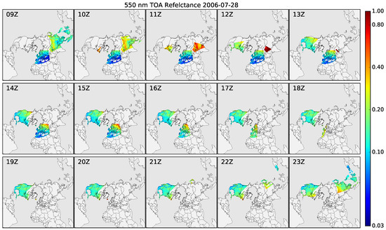
Figure 9.
Simulated 550 nm TOA reflectance as would be observed by the geostationary constellation over 15 h on 28 July 2006.
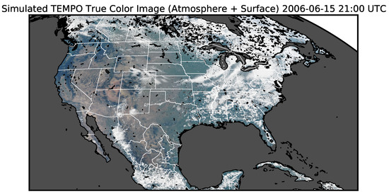
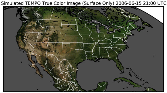
Figure 10.
Simulated true color image for 15 June 2006 21 UTC in the G5NR simulation as would be observed by TEMPO. The images were created by combining the simulated TOA reflectance at 470, 550, and 670 nm. The top image includes surface reflectance as well as atmospheric scattering from molecules, aerosols, and clouds. The bottom image shows surface reflectance alone.
Figure 11b shows a simulated true color image of a portion of the TEMPO domain covering the Northwest United States for the 20 UTC model time step on 27 July 2006. This image was created by combining the 470, 550, and 670 nm simulated TOA reflectance. Figure 11c,d also show the simulated 388 nm TOA reflectance, as well as the simulated ratio of 354 to 388 nm TOA reflectance. The TEMPO synthetic observations indicate several hot spots of enhanced 388 nm TOA reflectance corresponding to high aerosol concentrations from fires, which are apparent in the simulated true color image. These hotspots also correspond to lower values of 354:388 nm TOA reflectance ratio, indicating the presence of absorbing aerosol.
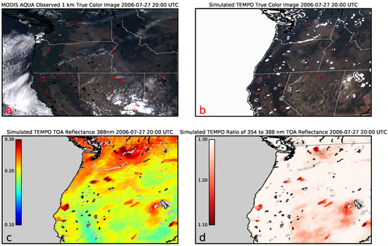
Figure 11.
(a) True color image observed by MODIS Aqua on July 7, 2006 at approximately 20 UTC created by combining the reflectance from channels 1, 3, and 4. (b) Simulated true color image for the same G5NR simulation day as would be observed by TEMPO, created by combining the simulated TOA reflectance at 470, 550, and 670 nm. In (a,b) the red squares represent the MODIS observed active fires (MCD14DL), which are used in G5NR to drive fire emissions calculated with QFED. (c) Simulated TOA reflectance at 388 nm, and (d) the ratio of simulated 354 nm to 388 nm TOA reflectance.
The locations of the simulated fires correspond with MODIS observed active fires for this day, as G5NR used the Quick Fire Emissions Database (QFED) [26] to simulate biomass burning. QFED uses the fire radiative power approach to estimate fire emissions, which relates time-integrated fire radiative energy to amount of fuel burned. Figure 11a shows the observed MODIS Aqua true color image for 27 July 2006 at approximately 20 UTC. Although the simulated and observed true color images indicate the same locations of fire hot spots and smoke emissions, as G5NR is not constrained by meteorological observations, the transport of the fire plume differs between the free running model and observations.
3.2. Application of Synthetic Observations to Study the Synergy between TEMPO and GOES-R
The GOES-R Series is a four-satellite program including GOES-R, GOES-S, GOES-T and GOES-U that will extend the operational GOES satellite system through 2036, and provide advanced imagery and atmospheric measurements of the Earth. The GOES-R Series will maintain the two-satellite operational system implemented by the current GOES satellites. The satellites will be located at 75.2° W and 137° W, providing excellent overlap with the TEMPO field of view. In addition, TEMPO and the GOES-R Series will complement each other in terms of spectral coverage. GOES-R measures 6 bands in the visible to near infrared (NIR) spectral range from 0.47 to 2.25 m, while TEMPO will provide spectral observations in the UV-Vis from 290 to 740 nm. Thus, there is an interest in studying how observations from the two platforms can be used synergistically. One application for the synergy of TEMPO and GOES-R observations is aerosol type detection. The combination of UV-Vis observations from TEMPO and NIR observations from GOES-R has the potential to provide aerosol type discrimination that may not be possible from observations from each sensor alone. In this section, we will describe how simulated observation data for a biomass burning and a dust event were used in a case study designed to demonstrate how future observations from TEMPO could be used in conjunction with simultaneous observations from GOES-R for aerosol type detection. Specifically, the focus for the two case studies was on (1) detecting smoke from the Pacific Northwest fires on 27 July 2006 in the G5NR simulation, and (2) detecting wind-blown dust coming from the Sonoran Desert on 13 May 2007 in the G5NR simulation.
3.2.1. Overview of the VIIRS Aerosol Detection Algorithm
The aerosol detection algorithm used in the case study was initially developed for the Visible Infrared Imaging Radiometer Suite (VIIRS), a key instrument on-board the Suomi National Polar-Orbiting Partnership (SNPP) spacecraft [58]. In the algorithm, the presence of absorbing aerosol is detected by a decrease in the spectral contrast between light reflected at two neighboring deep-blue wavelengths observed by VIIRS (412 nm and 440 nm) relative to a Rayleigh scattering only atmosphere. This spectral contrast is quantified by the Absorbing Aerosol Index (AAI), defined as:
where and are the observed TOA reflectance at 412 and 440 nm, respectively, and and are the TOA reflectance for a Rayleigh scattering atmosphere at 412 and 440 nm calculated with the 6S RTM [59] for the given location and satellite viewing geometry. Observations with large values of AAI indicate the presence of enhanced aerosol absorption.
Because of the large particle size, dust scatters radiation in the shortwave IR. This can be used to distinguish dust from other types of absorbing aerosol (i.e., smoke), which have small particle size and are mostly transparent in this spectral range. The dust smoke discrimination index (DSDI), defined in Equation (24), was developed to aid in separating the dust from smoke, and describes the spectral contrast between TOA reflectance at 412 nm () and 2250 nm (). Observations with large values of both AAI and DSDI indicate enhanced absorption and scattering by dust.
Optimal thresholds for AAI and DSDI that discriminate between cases of enhanced AOD of dust and smoke from clean atmosphere were determined by analyzing MODIS Aqua observations from 2002-2012 in which smoke and dust events could be identified (i.e., supervised training) [58]. Using these thresholds, the VIIRS aerosol detection algorithm flags pixels as smoke, dust, or clear/undetermined. The algorithm was validated with (1) the CALIOP Vertical Feature Mask product [60], which identifies aerosol types (including smoke and dust), and (2) AERONET inversion data, which provides Angstrom Exponent observations, from which aerosols with small particle size (smoke) and aerosols with large particle size (dust) aerosols can be identified [61,62]. The validation indicated that smoke and dust with AOD > 0.2 can be detected by the algorithm to within an accuracy of 80 and 70%, respectively [58].
The GOES-R Series instruments do not have observations in the deep-blue, as the shortest channel is 470 nm, precluding absorbing aerosol detection using the AAI. However, TEMPO will have measurements in the UV-Vis, though it will lack the short-wave IR observation needed to discriminate dust from smoke. Thus, a joint TEMPO/GOES-R aerosol type detection algorithm will be needed. The simulated observations derived from the G5NR simulation provide a unique dataset to study and demonstrate this potential synergy between GOES-R and TEMPO observations. For this end, we applied the VIIRS aerosol detection algorithm to the 412 nm and 440 nm simulated observations from TEMPO, and the 2250 nm observation from GOES-R. No modifications were made to the algorithm, which assumes that surface reflectance is Lambertian. In the next section we will show that this can lead to lower algorithm accuracy for the viewing geometries of TEMPO and GOES-R.
3.2.2. Case Study 1: Smoke Detection
The aerosol detection algorithm code was run using the 27 July 2006 simulated TOA reflectance data as inputs. The 412 nm and 440 nm simulated observations were derived for the TEMPO domain and viewing geometry, while the 2250 nm simulated observations were derived for the GOES-R domain and viewing geometry, assuming 137° W as the sub-satellite longitude. The GOES-R observations falling within each TEMPO pixel were averaged, such that the TOA reflectance at all three channels were on the same grid.
Figure 12 shows aerosol detection results for the simulated data on 27 July 2006 at 20 UTC, corresponding to afternoon for the western US. The shading in Figure 12a indicates the simulated AOD at 550 nm, and the purple curves outline the areas that were detected as smoke. Please note that only pixels with 550 nm AOD greater than 0.2 are shaded in the figures because this is the established detection limit for the aerosol detection algorithm [58]. The shading in Figure 12b indicates the contribution of smoke AOD (defined as the sum of BC and OC AOD) to the total model AOD. The figures show that the VIIRS aerosol detection algorithm identifies most areas of simulated dense smoke. This indicates that (1) the optical properties of the smoke aerosols in the G5NR simulation are consistent with the MODIS observations from which AAI thresholds were derived for the aerosol detection algorithm, and (2) combining TEMPO and GOES-R observations to characterize smoke aerosol is a viable strategy. However, Figure 13a shows that some missed detections of dense smoke, such as in northeast Nevada, occur even in areas with AAI greater than 5, the AAI threshold for identifying smoke. This is because the DSDI is above the threshold to distinguish dust from smoke (DSDI must be less than −3) (Figure 14a). Figure 14b shows that if the DSDI were calculated with hypothetical 2250 nm observations from the TEMPO viewpoint, i.e., the same viewing geometry as 412 nm reflectance, consistent with how the algorithm was developed, the DSDI would be below the threshold to identify smoke in most of the missed detection areas. The lower 2250 nm reflectance at the TEMPO geometry is strongly driven by reduced bidirectional surface reflectance in the simulations when going from the GOES-R to TEMPO viewing geometries (Figure 15). This effect is more significant where there is elevated surface reflectance (Figure 13b), as less of the TOA reflectance comes from aerosol scattering. For greater accuracy, re-training the algorithm thresholds, especially angular dependent thresholds, for the combined GOES-R and TEMPO viewing geometries is recommended.
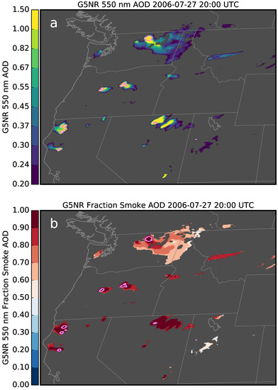
Figure 12.
(a) Simulated 550 nm AOD, (b) fraction of simulated 550 nm AOD coming from smoke for 27 July 2006 at 21 UTC in the G5NR simulation. The purple contours represent the areas that were detected as smoke by the VIIRS aerosol detection algorithm.
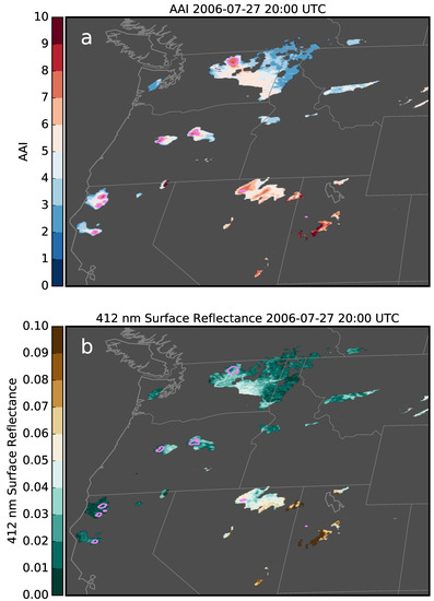
Figure 13.
(a) Simulated Aerosol Absorbing Index (AAI), (b) TEMPO 412 nm surface reflectance used for AAI and DSDI calculations for 27 July 2006 at 21 UTC in the G5NR simulation. The purple contours represent the areas that were detected as smoke by the VIIRS aerosol detection algorithm.
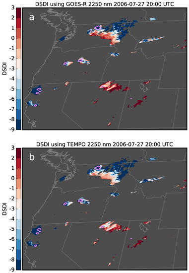
Figure 14.
(a) Simulated Dust-Smoke Discrimination Index (DSDI) using combined TEMPO 412 nm reflectance and GOES-R 2250 nm reflectance, (b) DSDI using only TEMPO 412 nm and 2250 nm reflectance for 27 July 2006 at 21 UTC in the G5NR simulation. The purple contours represent the areas that were detected as smoke by the VIIRS aerosol detection algorithm.
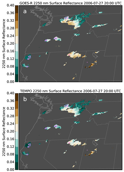
Figure 15.
(a) Simulated GOES-R 2250 nm surface reflectance re-gridded to the TEMPO resolution, and (b) TEMPO 2250 nm surface reflectance for 27 July 2006 at 21 UTC in the G5NR simulation. The purple contours represent the areas that were detected as smoke by the VIIRS aerosol detection algorithm.
Some missed smoke detections, such as the thin to moderately dense parts of the Washington state smoke plume that was transported away from the fire and mixed with other aerosol, occurred even over dark surfaces because the AAI was too low. As we know the true aerosol composition in each pixel, we can examine how the algorithm performs as a function of the contribution of smoke to the total AOD. The diurnal variation of the accuracy of the algorithm is shown in Figure 16. Accuracy is defined as:
where (true positive) is the number of pixels where the algorithm correctly detects smoke, (true negative) is the number of pixels where the algorithm correctly detects there is no smoke, (false positive) is the number of pixels where the algorithm falsely detects smoke, and is the number of pixels where smoke is present but the algorithm fails to detect it.
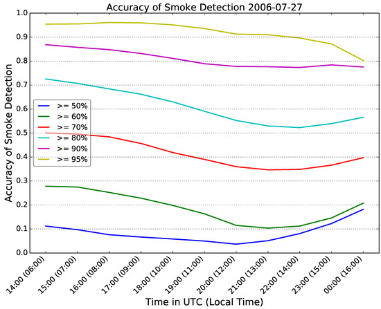
Figure 16.
Accuracy of smoke detection on 27 July 2006 (solid lines). The different colored lines represent the accuracy when a “true smoke” pixel is defined by different thresholds of the contribution of smoke to the total AOD. The highest accuracy occurs when only pixels with pure smoke (>95% of total AOD coming from smoke) are considered as “true smoke”.
Figure 16 indicates that the algorithm has the highest accuracy when only pixels with pure smoke (>95% of total AOD coming from smoke) are considered as “true smoke”. For this case, the accuracy of the retrieval is greater than 80%, in agreement with the results from the validation of the algorithm using real observations [58]. The diurnal variability in the accuracy of the algorithm is due to the fact that fire activity increases in the afternoon, which increases the number of missed detections.
3.2.3. Case 2: Dust Detection
On 13 May 2007 in the G5NR simulation, wind-blown dust coming from the Sonoran Desert led to elevated AOD in the area southwest of Phoenix, along the US-Mexico border. As before, the aerosol detection algorithm code was run using the simulated TEMPO and GOES-R TOA reflectance data for this day as inputs. The contour lines in Figure 17 outline the areas that are detected as containing dust at the 20 UTC simulation time step, the model hour with the highest dust AOD. The figure shows that the algorithm tends to underestimate the extent of the dust plume. Overlaying the dust detection contours over the surface reflectance RTM inputs (Figure 18) shows that the combination of low surface reflectance spectral contrast and high surface reflectance leads to elevated AAI that is interpreted by the algorithm as absorbing aerosol. This is a known uncertainty in the retrieval methodology, and is most relevant over bright surfaces and low dust optical thickness, where light reflected by the surface contributes significantly to TOA reflectance. This case study indicates that the detection threshold of dust over land is probably higher than the value of 0.2 that has been assumed before, as the accuracy for this case study was less than 50% for this day. The suggestion in Ciren and Kondragunta [58] of deriving AAI thresholds for different land surface types has merit and could improve the retrieval.
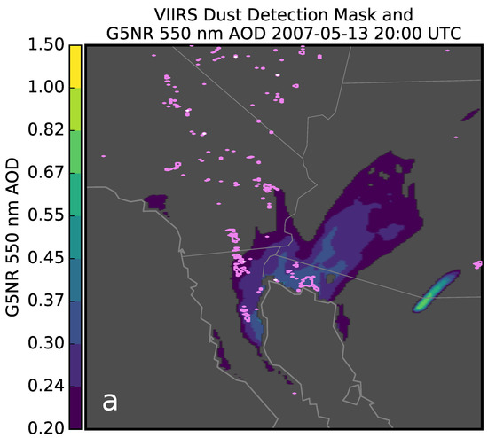
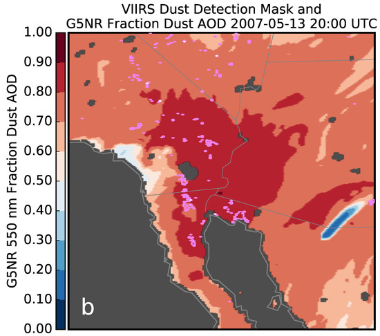
Figure 17.
(a) Simulated 550 nm AOD, (b) fraction of simulated 550 nm AOD coming from dust for 13 May 2007 at 20 UTC. The purple contours represent the areas that were detected as smoke by the VIIRS aerosol detection algorithm.
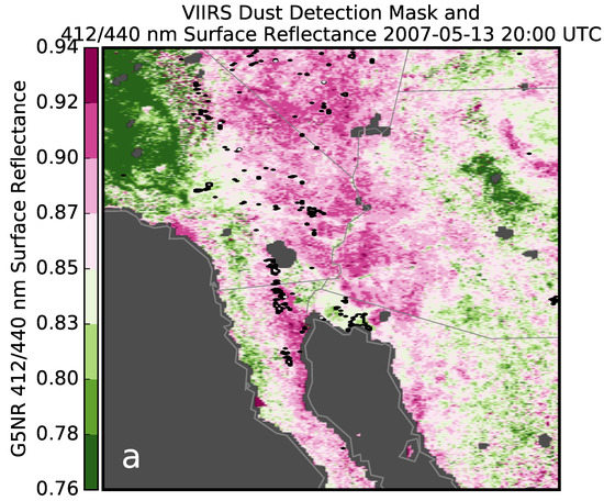
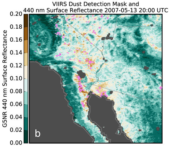
Figure 18.
(a) Ratio of simulated 412 nm to 440 nm surface reflectance, and (b) simulated 440 nm surface reflectance for 13 May 2007 at 20 UTC. The black and purple contours represent the areas that were detected as smoke by the VIIRS aerosol detection algorithm.
4. Concluding Remarks and Outlook
In this paper we described a detailed and accurate (less than 1.0% uncertainty) model for calculating TOA radiance from the GEOS-5 nature run for a constellation of geostationary sensors for observing air quality. The current generation of aerosol retrieval algorithms are optimized for specific conditions such as afternoon well-mixed atmospheres, and limited viewing and illumination angles. The G5NR and the simulated observations described in this document provide an opportunity to test these algorithms globally over a realistic dynamic range. A combined TEMPO and GOES-R retrieval algorithm for aerosol type detection based on empirical thresholds of aerosol index derived from MODIS observations was demonstrated and evaluated using the simulated observations. We found that the combination of UV-Vis observations from TEMPO and near-infrared observations from GOES-R can be used to accurately detect dense smoke. However, to achieve greater accuracy in aerosol detection, re-training the algorithm thresholds for the combined GOES-R and TEMPO viewing geometries is recommended as neglecting the difference in surface bidirectional reflectance between the different viewing angles can lead to missed detections. To improve dust detection, deriving aerosol index thresholds for different land surface types is recommended. This analysis coincidentally showed that the optical properties of the smoke aerosols in the simulated observations are consistent with the MODIS observations from which the aerosol index thresholds were derived.
There are many more potential applications for the simulated observations described in this paper, such as establishing new retrievals or instrument requirements during the development of new mission concepts. For example, the data will be used to prototype retrievals using polarized multi-angle and multi-channel observations spanning the UV and visible wavelengths, which have the potential to provide several pieces of information beyond AOD such as aerosol absorption and fine mode fraction. The synthetic observations will also be used to analyze how the new time resolved measurements and the increase in spatial coverage from geostationary orbit effects chemical weather forecasts and data analysis, particularly with respect to the current suite of LEO observations.
Future development of the instrument simulator capabilities will focus on including molecular absorption effects from water vapor and trace gases in the radiance calculation. This will be required for applications that use the hyperspectral feature of the new instruments. This will also require trace gas vertical profile inputs from a full chemistry nature run [63]. Furthermore, we are currently developing instrument simulator capabilities for ocean color instruments, such as PACE (Plankton, Aerosol, Cloud, ocean Ecosystem), that include detailed hyperspectral water leaving radiance calculations. These developments will provide the opportunity to test strategies for handling complex trace gas, aerosol, cloud, and surface interactions in retrieval algorithms [11,64,65].
Author Contributions
Conceptualization, P.C. (Patricia Castellanos), A.M.d.S., A.S.D. and S.K.; Data curation, P.C. (Patricia Castellanos), A.S.D., V.B., R.C.G. and P.C. (Pubu Ciren); Formal analysis, P.C. (Patricia Castellanos), A.S.D., V.B. and P.C. (Pubu Ciren); Funding acquisition, A.M.d.S. and S.K.; Investigation, P.C. (Patricia Castellanos) and P.C. (Pubu Ciren); Methodology, P.C. (Patricia Castellanos), A.M.d.S. and A.S.D.; Project administration, A.M.d.S.; Resources, A.M.d.S. and S.K.; Software, P.C. (Patricia Castellanos); Supervision, A.M.d.S. and S.K.; Validation, P.C. (Patricia Castellanos), A.S.D. and V.B.; Visualization, P.C. (Patricia Castellanos), A.S.D. and V.B.; Writing—original draft, P.C. (Patricia Castellanos), A.S.D. and P.C. (Pubu Ciren); Writing—review & editing, P.C. (Patricia Castellanos), A.M.d.S. and V.B.
Funding
This research was funded by the NASA GEO-CAPE pre-formulation study.
Conflicts of Interest
The authors declare no conflict of interest. The funding sponsors had no role in the design of the study; in the collection, analyses, or interpretation of data; in the writing of the manuscript, and in the decision to publish the results.
Appendix A. VLIDORT Benchmarking and TOA Radiance Uncertainty Estimate
Here we present uncertainty estimates of the vector radiative transfer calculations from VLIDORT by comparing TOA radiances calculated with VLIDORT to that of five other polarized radiative transfer models. Spurr [46] and Wang et al. [11] reported on benchmarking results against the solutions of Coulson et al. [66] and Siewert [67] for the Rayleigh and aerosol slab problems, respectively, and found that VLIDORT was able to reproduce their results to the reported level of accuracy of the benchmark datasets. In the following, VLIDORT is benchmarked for five additional scenarios, including realistic atmospheric profiles and spheroidal aerosol particles. Table A2 describes the seven scenarios that were considered, consisting of four single layer problems, and three 32-layer problems containing various configurations of Rayleigh scattering, aerosol scattering, and molecular absorption. For this analysis, VLIDORT was run in the same configuration as described in Section 2.4.2.
Table A1 lists the various RTMs considered in the intercomparison and their solution strategies, which were either discrete ordinates (similar to VLIDORT), or rigorous Monte Carlo solutions. In general, all models in Table A1 were run in high accuracy mode (e.g., 128 streams for spheroidal aerosol cases), and the results provide a good dataset for analyzing the accuracy of the low (6) stream VLIDORT approximation. Details of each model can be found in Emde et al. [68], and the model outputs for all scenarios were downloaded from the following website: http://www.meteo.physik.uni-muenchen.de/~iprt/doku.php?id=intercomparisons:intercomparisons.
Table A1.
Benchmark intercomparison polarized radiative transfer models.
Table A1.
Benchmark intercomparison polarized radiative transfer models.
| Name | Solution Method | Reference |
|---|---|---|
| MYSTIC | Monte Carlo | Mayer [69] Emde et al. [70] |
| PSTAR | Discrete Ordinate | Ota et al. [71] |
| SPARTA | Monte Carlo | Barlakas et al. [72] |
| SHDOM | Discrete Ordinate | Evans [73] |
| IPOL | Discrete Ordinate | ftp://climate1.gsfc.nasa.gov/skorkin/IPOL |
Table A2.
Benchmark intercomparison scenarios. Viewing zenith angles range from 0° to 80° with an increment of 5°. Viewing azimuth angles range from 0° to 360° with an increment of 5°.
Table A2.
Benchmark intercomparison scenarios. Viewing zenith angles range from 0° to 80° with an increment of 5°. Viewing azimuth angles range from 0° to 360° with an increment of 5°.
| Scenario Name | Description |
|---|---|
| A1 | Rayleigh Slab |
| Optical Thickness = 0.5 | |
| Surface Albedo = 0.0 | |
| Case 1: SZA = 0°, SAA = 65°, Depolarization Factor = 0.00 | |
| Case 2: SZA = 30°, SAA = 0°, Depolarization Factor = 0.03 | |
| Case 3: SZA = 30°, SAA = 65°, Depolarization Factor = 0.10 | |
| A2 | Rayleigh Slab over a Lambertian Surface |
| Optical Thickness = 0.1 | |
| Surface Albedo = 0.3 | |
| Depolarization Factor = 0.03 | |
| SZA = 50°, SAA = 0° | |
| A3 | Aerosol Slab—Spherical Particles |
| AOD = 0.2 | |
| Surface Albedo = 0.0 | |
| Phase matrix corresponds to water soluble aerosol at 50% RH from OPAC database | |
| SZA = 30°, SAA = 0° | |
| A4 | Aerosol Slab—Spheroidal Particles |
| AOD = 0.2 | |
| Surface Albedo = 0.0 | |
| Phase matrix corresponds to prolate spheroid with aspect ratio of 3.0 | |
| SZA = 40°, SAA = 0° | |
| B1 | Rayleigh Scattering Vertical Profile—Standard Atmosphere |
| Rayleigh optical thickness profile typical of 450 nm | |
| Surface Albedo = 0.0 | |
| Depolarization Factor = 0.03 | |
| SZA = 60°, SAA = 0° | |
| B2 | Rayleigh Scattering and Molecular Absorption Vertical Profile—Standard Atmosphere |
| Rayleigh optical thickness and molecular absorption profile typical of 325 nm | |
| Surface Albedo = 0.0 | |
| Depolarization Factor = 0.03 | |
| SZA = 60°, SAA = 0° | |
| B3 | Aerosol Vertical Profile - Standard Atmosphere |
| Rayleigh optical thickness and molecular absorption profile typical of 350 nm | |
| Profile of spheroidal aerosols (same as scenario A4) | |
| Surface Albedo = 0.0 | |
| Depolarization Factor = 0.03 | |
| SZA = 30°, SAA = 0° |
Figure A1 shows the difference between VLIDORT and the Monte Carlo model, MYSTIC, which is generally the median the of the five benchmark models, for the aerosol vertical profile scenario (B3). The VLIDORT solutions fall within the 2-sigma uncertainty reported by the Monte Carlo RTM for nearly all scattering geometries. Table A3 shows the root mean square error between VLIDORT and the six benchmark RTMs for all seven radiative transfer scenarios considered. For all the benchmark scenarios the VLIDORT 6 stream approximation generally agrees to within at least 0.1% of most models. The largest mean error between the benchmark models and VLIDORT is 0.68%, which is comparable to the measurement errors in the UV-Vis for sensors such as OMI [74].
Table A3.
Root mean square error (RMSE) and relative RMSE (shown in parenthesis) between VLIDORT and the intercomparison RTMs for reflected total intensity. The values in the row labeled Average represent the RMSE between VLIDORT and the average of all the models.
Table A3.
Root mean square error (RMSE) and relative RMSE (shown in parenthesis) between VLIDORT and the intercomparison RTMs for reflected total intensity. The values in the row labeled Average represent the RMSE between VLIDORT and the average of all the models.
| Scenarios | Models | |||||
|---|---|---|---|---|---|---|
| MYSTIC | IPOL | SPARTA | PSTAR | SHDOM3 | Average | |
| A1 Case 1 | (0.02%) | (0.01%) | (0.05%) | (0.01%) | (0.04%) | (0.01%) |
| A1 Case 2 | (0.02%) | (0.01%) | (0.12%) | (0.01%) | (0.04%) | (0.02%) |
| A1 Case 3 | (0.02%) | (0.01%) | (0.16%) | (0.01%) | (0.04%) | (0.03%) |
| A2 | (0.01%) | (0.01%) | (0.01%) | (0.01%) | (0.06%) | (0.02%) |
| A3 | (0.11%) | (0.09%) | (0.11%) | (0.09%) | (0.18%) | (0.10%) |
| A4 | (0.67%) | (0.68%) | (0.68%) | (0.68%) | (0.68%) | (0.68%) |
| B1 | (0.05%) | (0.05%) | (0.04%) | (0.05%) | (0.10%) | (0.06%) |
| B2 | (0.01%) | (0.004%) | (0.01%) | (0.004%) | (0.05%) | (0.01%) |
| B3 | (0.01%) | (0.01%) | (0.02%) | (0.01%) | (0.06%) | (0.02%) |

Figure A1.
Difference in total intensity between VLIDORT and MYSITC for the aerosol profile scenario (B3). The gray lines represent the 2-sigma uncertainty reported by MYSTIC, a Monte Carlo RTM.
Figure A1.
Difference in total intensity between VLIDORT and MYSITC for the aerosol profile scenario (B3). The gray lines represent the 2-sigma uncertainty reported by MYSTIC, a Monte Carlo RTM.

References
- Zoogman, P.; Liu, X.; Suleiman, R.M.; Pennington, W.F.; Flittner, D.E.; Al-Saadi, J.A.; Hilton, B.B.; Nicks, D.K.; Newchurch, M.J.; Carr, J.L.; et al. Tropospheric emissions: Monitoring of pollution (TEMPO). J. Quant. Spectrosc. Radiat. Transf. 2017, 186, 17–39. [Google Scholar] [CrossRef]
- Ingmann, P.; Veihelmann, B.; Langen, J.; Lamarre, D.; Stark, H.; Courrèges-Lacoste, G.B. Requirements for the GMES Atmosphere Service and ESA’s implementation concept: Sentinels-4/-5 and -5p. Remote Sens. Environ. 2012, 120, 58–69. [Google Scholar] [CrossRef]
- Bak, J.; Kim, J.H.; Liu, X.; Chance, K.; Kim, J. Evaluation of ozone profile and tropospheric ozone retrievals from GEMS and OMI spectra. Atmos. Meas. Tech. 2013, 6, 239–249. [Google Scholar] [CrossRef]
- Uno, I.; Eguchi, K.; Yumimoto, K.; Takemura, T.; Shimizu, A.; Uematsu, M.; Liu, Z.; Wang, Z.; Hara, Y.; Sugimoto, N. Asian dust transported one full circuit around the globe. Nat. Geosci. 2009, 2, 557–560. [Google Scholar] [CrossRef]
- Pérez, C.; Nickovic, S.; Pejanovic, G.; Baldasano, J.M.; Özsoy, E. Interactive dust-radiation modeling: A step to improve weather forecasts. J. Geophys. Res. Atmos. 2006, 111, 977. [Google Scholar] [CrossRef]
- Sokolik, I.N.; Toon, O.B. Direct radiative forcing by anthropogenic airborne mineral aerosols. Nature 1996, 381, 681–683. [Google Scholar] [CrossRef]
- Seinfeld, J.H.; Carmichael, G.R.; Arimoto, R.; Conant, W.C.; Brechtel, F.J.; Bates, T.S.; Cahill, T.A.; Clarke, A.D.; Doherty, S.J.; Flatau, P.J.; et al. ACE-ASIA: Regional Climatic and Atmospheric Chemical Effects of Asian Dust and Pollution. Bull. Am. Meteorol. Soc. 2004, 85, 367–380. [Google Scholar] [CrossRef]
- Li, L.; Sokolik, I.N. The Dust Direct Radiative Impact and Its Sensitivity to the Land Surface State and Key Minerals in the WRF-Chem-DuMo Model: A Case Study of Dust Storms in Central Asia. J. Geophys. Res. Atmos. 2018, 123, 4564–4582. [Google Scholar] [CrossRef]
- Sassen, K.; DeMott, P.J.; Prospero, J.M.; Poellot, M.R. Saharan dust storms and indirect aerosol effects on clouds: CRYSTAL-FACE results. Geophys. Res. Lett. 2003, 30, 1199. [Google Scholar] [CrossRef]
- Coopman, Q.; Garrett, T.J.; Finch, D.P.; Riedi, J. High Sensitivity of Arctic Liquid Clouds to Long-Range Anthropogenic Aerosol Transport. Geophys. Res. Lett. 2018, 45, 372–381. [Google Scholar] [CrossRef]
- Wang, J.; Xu, X.; Ding, S.; Zeng, J.; Spurr, R.; Liu, X.; Chance, K.; Mishchenko, M. A numerical testbed for remote sensing of aerosols, and its demonstration for evaluating retrieval synergy from a geostationary satellite constellation of GEO-CAPE and GOES-R. J. Quant. Spectrosc. Radiat. Transf. 2014, 146, 510–528. [Google Scholar] [CrossRef]
- Putman, W.; da Silva, A.; Ott, L.E.; Darmenov, A. Model Configuration for the 7-km GEOS-5 Nature Run, Ganymed Release; Technical Report GMAO Office Note No 5 (Version 1.0); Goddard Space Flight Center, National Aeronautics and Space Administration: Pasadena, CA, USA, 2014.
- Gelaro, R.; Putman, W.; Pawson, S.; Draper, C.; Molod, A.; Norris, P.M.; Ott, L.E.; Prive, N.; Reale, O.; Achuthavarier, D.; et al. Evaluation of the 7-km GEOS-5 Nature Run; Technical Report NASA/TM-2014-104606; Goddard Space Flight Center, National Aeronautics and Space Administration: Pasadena, CA, USA, 2015.
- Edwards, D.P.; Arellano, A.F.J.; Deeter, M.N. A satellite observation system simulation experiment for carbon monoxide in the lowermost troposphere. J. Geophys. Res. Atmos. 2009, 114. [Google Scholar] [CrossRef]
- Zoogman, P.; Jacob, D.J.; Chance, K.; Zhang, L.; Le Sager, P.; Fiore, A.M.; Eldering, A.; Liu, X.; Natraj, V.; Kulawik, S.S. Ozone air quality measurement requirements for a geostationary satellite mission. Atmos. Environ. 2011, 45, 7143–7150. [Google Scholar] [CrossRef]
- Claeyman, M.; Attié, J.L.; Peuch, V.H.; El Amraoui, L.; Lahoz, W.A.; Josse, B.; Joly, M.; Barré, J.; Ricaud, P.; Massart, S.; et al. A thermal infrared instrument onboard a geostationary platform for CO and O3 measurements in the lowermost troposphere: Observing System Simulation Experiments (OSSE). Atmos. Meas. Tech. 2011, 4, 1637–1661. [Google Scholar] [CrossRef]
- Barré, J.; Edwards, D.; Worden, H.; da Silva, A.; Lahoz, W. On the feasibility of monitoring carbon monoxide in the lower troposphere from a constellation of Northern Hemisphere geostationary satellites. (Part 1). Atmos. Environ. 2015, 113, 63–77. [Google Scholar] [CrossRef]
- Timmermans, R.M.A.; Schaap, M.; Builtjes, P.; Elbern, H.; Siddans, R.; Tjemkes, S.; Vautard, R. An Observing System Simulation Experiment (OSSE) for Aerosol Optical Depth from Satellites. J. Atmos. Ocean. Technol. 2009, 26, 2673–2682. [Google Scholar] [CrossRef]
- Chin, M.; Ginoux, P.; Kinne, S.; Torres, O.; Holben, B.N.; Duncan, B.N.; Martin, R.V.; Logan, J.A.; Higurashi, A.; Nakajima, T. Tropospheric Aerosol Optical Thickness from the GOCART Model and Comparisons with Satellite and Sun Photometer Measurements; American Meteorological Society: Boston, MA, USA, 2002. [Google Scholar] [CrossRef]
- Colarco, P.; da Silva, A.; Chin, M.; Diehl, T. Online simulations of global aerosol distributions in the NASA GEOS-4 model and comparisons to satellite and ground-based aerosol optical depth. J. Geophys. Res. Atmos. 2010, 115. [Google Scholar] [CrossRef]
- Randles, C.A.; da Silva, A.M.; Buchard, V.; Colarco, P.R.; Darmenov, A.; Govindaraju, R.; Smirnov, A.; Holben, B.; Ferrare, R.; Hair, J.; et al. The MERRA-2 Aerosol Reanalysis, 1980 Onward. Part I: System Description and Data Assimilation Evaluation. J. Clim. 2017, 30, 6823–6850. [Google Scholar] [CrossRef]
- Olivier, J.G.J.; Bouwman, A.F.; van der Maas, C.W.M.; Berdowski, J.J.M. Emission database for global atmospheric research (Edgar). Environ. Monit. Assess. 1994, 31, 93–106. [Google Scholar] [CrossRef]
- Janssens-Maenhout, G.; Dentener, F.; van Aardenne, J.; Monni, S.; Pagliari, V.; Orlandini, L.; Klimont, Z.; Kurokawa, J.i.; Akimoto, H.; Ohara, T.; et al. EDGAR-HTAP: A Harmonized Gridded Air Pollution Emissoin Dataset Based on National Inventories; Technical Report EUR 25229; European Commissions Joint Research Centre Institute for Environment and Sustainability: Luxembourg, 2012. [Google Scholar]
- Myhre, G.; Samset, B.H.; Schulz, M.; Balkanski, Y.; Bauer, S.; Berntsen, T.K.; Bian, H.; Bellouin, N.; Chin, M.; Diehl, T.; et al. Radiative forcing of the direct aerosol effect from AeroCom Phase II simulations. Atmos. Chem. Phys. 2013, 13, 1853–1877. [Google Scholar] [CrossRef]
- Lana, A.; Bell, T.G.; Simó, R.; Vallina, S.M.; Ballabrera-Poy, J.; Kettle, A.J.; Dachs, J.; Bopp, L.; Saltzman, E.S.; Stefels, J.; Johnson, J.E.; et al. An updated climatology of surface dimethlysulfide concentrations and emission fluxes in the global ocean. Glob. Biogeochem. Cycles 2011, 25. [Google Scholar] [CrossRef]
- Darmenov, A.; da Silva, A.M. The Quick Fire Emissions Dataset (QFED): Documentation of Versions 2.1, 2.2 and 2.4; Technical Report NASA/TM2015104606; Global Modeling and Assimilation Office, NASA Goddard Space Flight Center: Greenbelt, MD, USA, 2015.
- Kaiser, J.W.; Heil, A.; Andreae, M.O.; Benedetti, A.; Chubarova, N.; Jones, L.; Morcrette, J.J.; Razinger, M.; Schultz, M.G.; Suttie, M.; et al. Biomass burning emissions estimated with a global fire assimilation system based on observed fire radiative power. Biogeosciences 2012, 9, 527–554. [Google Scholar] [CrossRef]
- Duncan, B.N.; Strahan, S.E.; Yoshida, Y.; Steenrod, S.D.; Livesey, N. Model study of the cross-tropopause transport of biomass burning pollution. Atmos. Chem. Phys. 2007, 7, 3713–3736. [Google Scholar] [CrossRef]
- Strahan, S.E.; Duncan, B.N.; Hoor, P. Observationally derived transport diagnostics for the lowermost stratosphere and their application to the GMI chemistry and transport model. Atmos. Chem. Phys. 2007, 7, 2435–2445. [Google Scholar] [CrossRef]
- Strahan, S.E.; Douglass, A.R.; Newman, P.A. The contributions of chemistry and transport to low arctic ozone in March 2011 derived from Aura MLS observations. J. Geophys. Res. Atmos. 2013, 118, 1563–1576. [Google Scholar] [CrossRef]
- Buchard, V.; da Silva, A.M.; Colarco, P.R.; Darmenov, A.; Randles, C.A.; Govindaraju, R.; Torres, O.; Campbell, J.; Spurr, R. Using the OMI aerosol index and absorption aerosol optical depth to evaluate the NASA MERRA Aerosol Reanalysis. Atmos. Chem. Phys. 2015, 15, 5743–5760. [Google Scholar] [CrossRef]
- Textor, C.; Schulz, M.; Guibert, S.; Kinne, S.; Balkanski, Y.; Bauer, S.; Berntsen, T.; Berglen, T.; Boucher, O.; Chin, M.; et al. Analysis and quantification of the diversities of aerosol life cycles within AeroCom. Atmos. Chem. Phys. 2006, 6, 1777–1813. [Google Scholar] [CrossRef]
- Winker, D.M.; Pelon, J.; Coakley, J.A., Jr.; Ackerman, S.A.; Charlson, R.J.; Colarco, P.R.; Flamant, P.; Fu, Q.; Hoff, R.M.; Kittaka, C.; et al. The CALIPSO Mission: A Global 3D View of Aerosols and Clouds. Bull. Am. Meteorol. Soc. 2010, 91, 1211–1229. [Google Scholar] [CrossRef]
- Grigas, T.; Hervo, M.; Gimmestad, G.; Forrister, H.; Schneider, P.; Preißler, J.; Tarrason, L.; O’Dowd, C. CALIOP near-real-time backscatter products compared to EARLINET data. Atmos. Chem. Phys. 2015, 15, 12179–12191. [Google Scholar] [CrossRef]
- Lucht, W.; Schaaf, C.B.; Strahler, A.H. An algorithm for the retrieval of albedo from space using semiempirical BRDF models. IEEE Trans. Geosci. Remote Sens. 2000, 38, 977–998. [Google Scholar] [CrossRef]
- Li, X.; Strahler, A.H. Geometric-optical bidirectional reflectance modeling of the discrete crown vegetation canopy: Effect of crown shape and mutual shadowing. IEEE Trans. Geosci. Remote Sens. 1992, 30, 276–292. [Google Scholar] [CrossRef]
- Roujean, J.L.; Leroy, M.; Deschanps, P.Y. A Bidirectional Reflectance Model of the Earth’s Surface for the Correction of Remote Sensing Data. J. Geophys. Res. 1992, 97, 20455–20468. [Google Scholar] [CrossRef]
- Lyapustin, A.; Martonchik, J.; Wang, Y.; Laszlo, I.; Korkin, S. Multiangle implementation of atmospheric correction (MAIAC): 1. Radiative transfer basis and look-up tables. J. Geophys. Res. Atmos. 2011, 116, D03210. [Google Scholar] [CrossRef]
- Lyapustin, A.; Wang, Y.; Laszlo, I.; Kahn, R.; Korkin, S.; Remer, L.; Levy, R.; Reid, J.S. Multiangle implementation of atmospheric correction (MAIAC): 2. Aerosol algorithm. J. Geophys. Res. Atmos. 2011, 116, D03211. [Google Scholar] [CrossRef]
- Norris, P.M.; Oreopoulos, L.; Hou, A.Y.; Tao, W.K.; Zeng, X. Representation of 3D heterogeneous cloud fields using copulas: Theory for water clouds. Q. J. R. Meteorol. Soc. 2008, 134, 1843–1864. [Google Scholar] [CrossRef]
- Norris, P.M.; da Silva, A.M. Monte Carlo Bayesian inference on a statistical model of sub-gridcolumn moisture variability using high-resolution cloud observations. Part 1: Method. Q. J. R. Meteorol. Soc. 2016, 142, 2505–2527. [Google Scholar] [CrossRef] [PubMed]
- Wind, G.; da Silva, A.M.; Norris, P.M.; Platnick, S. Multi-sensor cloud retrieval simulator and remote sensing from model parameters—Part 1: Synthetic sensor radiance formulation. Geosci. Model Dev. 2013, 6, 2049–2062. [Google Scholar] [CrossRef]
- Spurr, R. VLIDORT: A linearized pseudo-spherical vector discrete ordinate radiative transfer code for forward model and retrieval studies in multilayer multiple scattering media. J. Quant. Spectrosc. Radiat. Transf. 2006, 102, 316–342. [Google Scholar] [CrossRef]
- Baum, B.A.; Heymsfield, A.J.; Yang, P.; Bedka, S.T. Bulk Scattering Properties for the Remote Sensing of Ice Clouds. Part I: Microphysical Data and Models. J. Appl. Meteorol. 2005, 44, 1885–1895. [Google Scholar] [CrossRef]
- Mishchenko, M.I.; Lacis, A.A.; Travis, L.D. Errors induced by the neglect of polarization in radiance calculations for rayleigh-scattering atmospheres. J. Quant. Spectrosc. Radiat. Transf. 1994, 51, 491–510. [Google Scholar] [CrossRef]
- Spurr, R. LIDORT and VLIDORT: Linearized pseudo-spherical scalar and vector discrete ordinate radiative transfer models for use in remote sensing retrieval problems. In Light Scattering Reviews 3; Springer: Berlin/Heidelberg, Geramny, 2008; pp. 229–275. [Google Scholar]
- Bodhaine, B.A.; Wood, N.B.; Dutton, E.G.; Slusser, J.R. On Rayleigh Optical Depth Calculations. J. Atmos. Ocean. Technol. 1999, 16, 1854–1861. [Google Scholar] [CrossRef]
- Tomasi, C.; Vitale, V.; Petkov, B.; Lupi, A.; Cacciari, A. Improved algorithm for calculations of Rayleigh-scattering optical depth in standard atmospheres. Appl. Opt. 2005, 44, 3320. [Google Scholar] [CrossRef] [PubMed]
- Gong, S.L. A parameterization of sea-salt aerosol source function for sub- and super-micron particles. Glob. Biogeochem. Cycles 2003, 17. [Google Scholar] [CrossRef]
- Koepke, P.; Hess, M.; Schult, I.; Shettle, E.P. Global Aerosol Data Set; Technical Report 243; MPI Meteorologie: Hamburg, Germany, 1997. [Google Scholar]
- Gong, S.L.; Barrie, L.A.; Blanchet, J.P. Modeling sea-salt aerosols in the atmosphere: 1. Model development. J. Geophys. Res. Atmos. 1997, 102, 3805–3818. [Google Scholar] [CrossRef]
- Wiscombe, W.J. Improved Mie scattering algorithms. Appl. Opt. 1980, 19, 1505–1509. [Google Scholar] [CrossRef]
- Hess, M.; Koepke, P.; Schult, I. Optical Properties of Aerosols and Clouds: The Software Package OPAC. Bull. Am. Meteorol. Soc. 1998, 79, 831–844. [Google Scholar] [CrossRef]
- Meng, Z.; Yang, P.; Kattawar, G.W.; Bi, L.; Liou, K.N.; Laszlo, I. Single-scattering properties of tri-axial ellipsoidal mineral dust aerosols: A database for application to radiative transfer calculations. J. Aerosol Sci. 2010, 41, 501–512. [Google Scholar] [CrossRef]
- Colarco, P.R.; Nowottnick, E.P.; Randles, C.A.; Yi, B.; Yang, P.; Kim, K.M.; Smith, J.A.; Bardeen, C.G. Impact of radiatively interactive dust aerosols in the NASA GEOS-5 climate model: Sensitivity to dust particle shape and refractive index. J. Geophys. Res. Atmos. 2014, 119, 753–786. [Google Scholar] [CrossRef]
- Shettle, E.P.; Fenn, R.W. Models for the Aerosols of the Lower Atmosphere and Effects of Humidity Variation on Their Optical Properties; Technical Report AFGL-TR-79-0214; Air Force Geophysics Laboratory: Hanscom AFB, MA, USA, 1979. [Google Scholar]
- Kim, D.; Chin, M.; Yu, H.; Eck, T.F.; Sinyuk, A.; Smirnov, A.; Holben, B.N. Dust optical properties over North Africa and Arabian Peninsula derived from the AERONET dataset. Atmos. Chem. Phys. 2011, 11, 10733–10741. [Google Scholar] [CrossRef]
- Ciren, P.; Kondragunta, S. Dust aerosol index (DAI) algorithm for MODIS. J. Geophys. Res. Atmos. 2014, 119, 4770–4792. [Google Scholar] [CrossRef]
- Kotchenova, S.Y.; Vermote, E.F.; Matarrese, R.; Klemm, F.J., Jr. Validation of a vector version of the 6S radiative transfer code for atmospheric correction of satellite data Part I: Path radiance. Appl. Opt. 2006, 45, 6762–6774. [Google Scholar] [CrossRef] [PubMed]
- Winker, D.M.; Vaughan, M.A.; Omar, A.; Hu, Y.; Powell, K.A.; Liu, Z.; Hunt, W.H.; Young, S.A. Overview of the CALIPSO Mission and CALIOP Data Processing Algorithms. J. Atmos. Ocean. Technol. 2009, 26, 2310–2323. [Google Scholar] [CrossRef]
- Dubovik, O.; Holben, B.; Eck, T.F.; Smirnov, A.; Kaufman, Y.J.; King, M.D.; Tanré, D.; Slutsker, I. Variability of Absorption and Optical Properties of Key Aerosol Types Observed in Worldwide Locations. J. Atmos. Sci. 2002, 59, 590–608. [Google Scholar] [CrossRef]
- Dubovik, O.; Sinyuk, A.; Lapyonok, T.; Holben, B.N.; Mishchenko, M.; Yang, P.; Eck, T.F.; Volten, H.; Muñoz, O.; Veihelmann, B.; et al. Application of spheroid models to account for aerosol particle nonsphericity in remote sensing of desert dust. J. Geophys. Res. 2006, 111, 156. [Google Scholar] [CrossRef]
- Hu, L.; Keller, C.A.; Long, M.S.; Sherwen, T.; Auer, B.; da Silva, A.; Nielsen, J.E.; Pawson, S.; Thompson, M.A.; Trayanov, A.L.; et al. Global simulation of tropospheric chemistry at 12.5 km resolution: Performance and evaluation of the GEOS-Chem chemical module (v10-1) within the NASA GEOS Earth system model (GEOS-5 ESM). Geosci. Model Dev. 2018, 11, 4603–4620. [Google Scholar] [CrossRef]
- Lin, J.T.; Liu, Z.; Zhang, Q.; Liu, H.; Mao, J.; Zhuang, G. Modeling uncertainties for tropospheric nitrogen dioxide columns affecting satellite-based inverse modeling of nitrogen oxides emissions. Atmos. Chem. Phys. 2012, 12, 12255–12275. [Google Scholar] [CrossRef]
- Castellanos, P.; Boersma, K.F.; Torres, O.; de haan, J.F. OMI tropospheric NO2 air mass factors over South America: Effects of biomass burning aerosols. Atmos. Meas. Tech. 2015, 8, 3831–3849. [Google Scholar] [CrossRef]
- Coulson, K.L.; Dave, J.V.; Sekera, Z. Tables Related to Radiation Emerging from a Planetary Atmosphere with Rayleigh Scattering; University of California Press: Berkeley, CA, USA, 1960. [Google Scholar]
- Siewert, C.E. A discrete-ordinates solution for radiative-transfer models that include polarization effects. J. Quant. Spectrosc. Radiat. Transf. 2000, 64, 227–254. [Google Scholar] [CrossRef]
- Emde, C.; Barlakas, V.; Cornet, C.; Evans, F. IPRT polarized radiative transfer model intercomparison project—Phase A. J. Quant. Spectrosc. Radiat. Transf. 2015, 209, 19–44. [Google Scholar] [CrossRef]
- Mayer, B. Radiative transfer in the cloudy atmosphere. Eur. Phys. J. Conf. 2009, 1, 75–99. [Google Scholar] [CrossRef]
- Emde, C.; Buras, R.; Mayer, B.; Blumthaler, M. The impact of aerosols on polarized sky radiance: Model development, validation, and applications. Atmos. Chem. Phys. 2010, 10, 383–396. [Google Scholar] [CrossRef]
- Ota, Y.; Higurashi, A.; Nakajima, T.; Yokota, T. Matrix formulations of radiative transfer including the polarization effect in a coupled atmosphere—Ocean system. J. Quant. Spectrosc. Radiat. Transf. 2010, 111, 878–894. [Google Scholar] [CrossRef]
- Barlakas, V.; Macke, A.; Wendisch, M. SPARTA—Solver for Polarized Atmospheric Radiative Transfer Applications: Introduction and application to Saharan dust fields. J. Quant. Spectrosc. Radiat. Transf. 2016, 178, 77–92. [Google Scholar] [CrossRef]
- Evans, K.F. The Spherical Harmonics Discrete Ordinate Method for Three-Dimensional Atmospheric Radiative Transfer. J. Atmos. Sci. 1998, 55, 429–446. [Google Scholar] [CrossRef]
- Liu, X.; Bhartia, P.K.; Chance, K.; Spurr, R.J.D.; Kurosu, T.P. Ozone profile retrievals from the Ozone Monitoring Instrument. Atmos. Chem. Phys. 2010, 10, 2521–2537. [Google Scholar] [CrossRef]


© 2018 by the authors. Licensee MDPI, Basel, Switzerland. This article is an open access article distributed under the terms and conditions of the Creative Commons Attribution (CC BY) license (http://creativecommons.org/licenses/by/4.0/).