Filling Gaps in Hourly Air Temperature Data Using Debiased ERA5 Data

Abstract
1. Introduction
2. Experiments
2.1. Data Set Description
2.1.1. ERA5 Reanalysis Data
2.1.2. Measured Weather Data
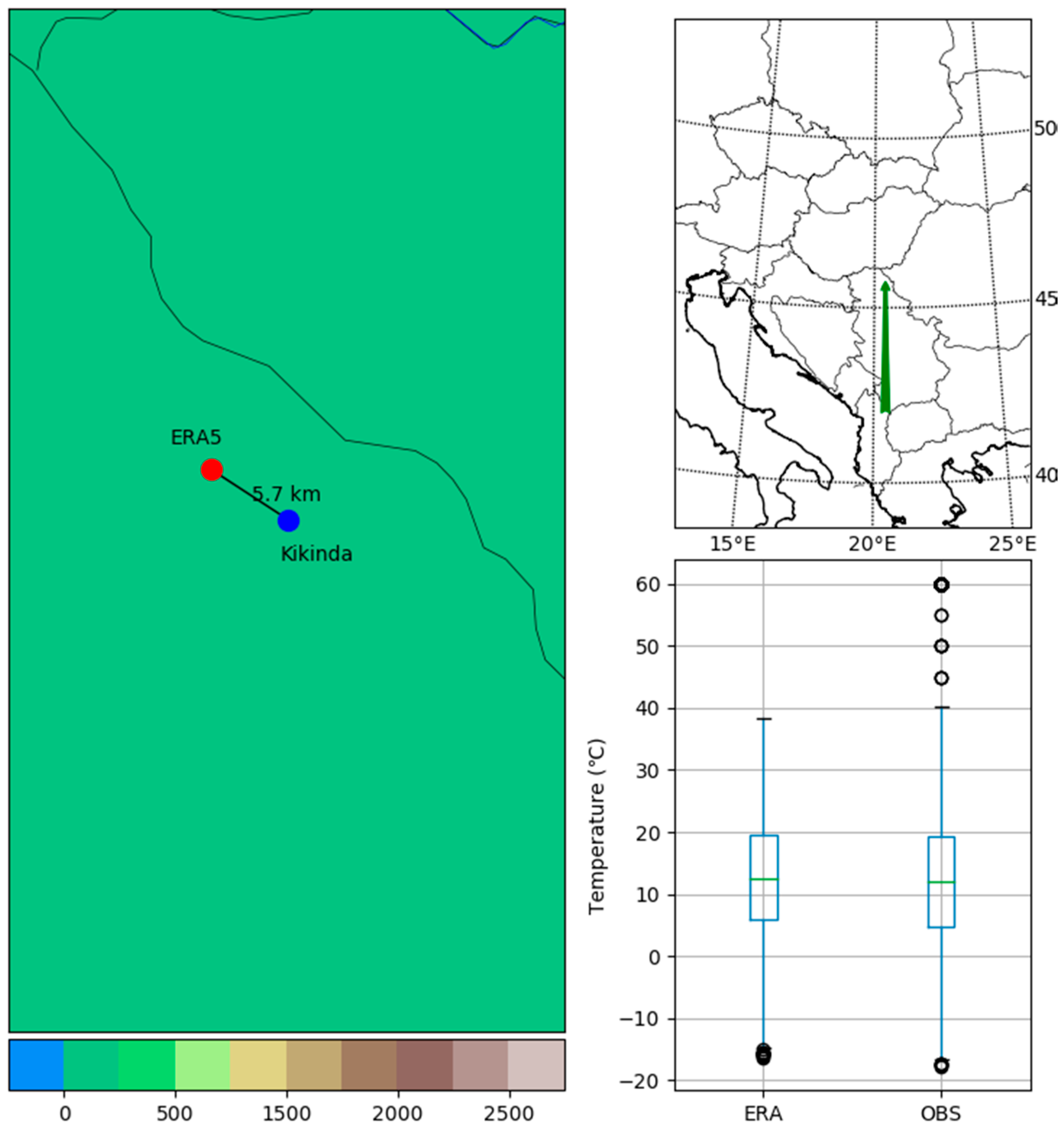
- Canopy measurements due to the impact of plants on micrometeorological conditions that cannot be identified by ERA5 due to the resolution of the land use map and the model itself;
- Mountain regions due to difficulties resulting from the distribution of orography over grid elements and the representation of mountains in the model used to produce ERA5 data;
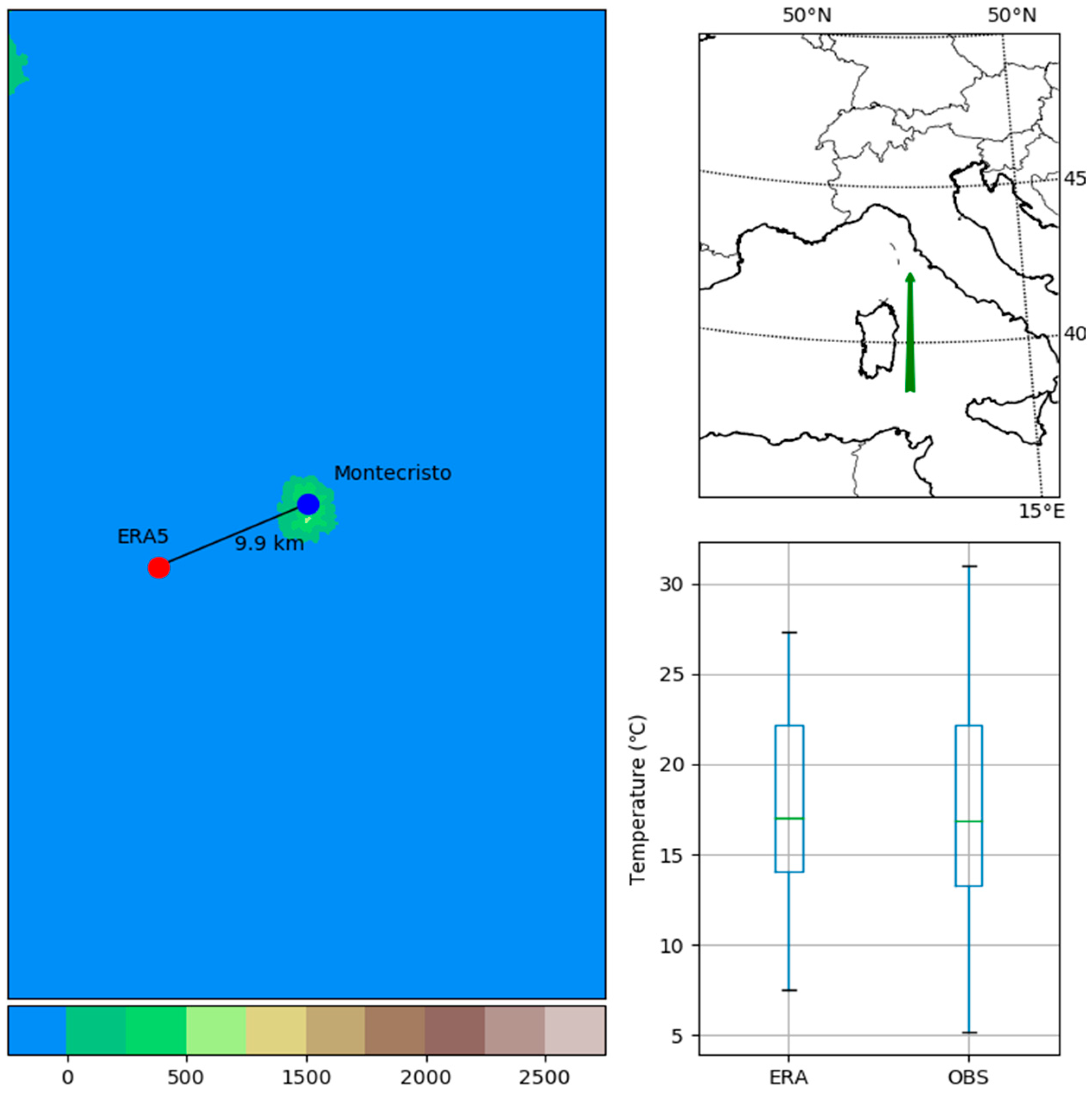
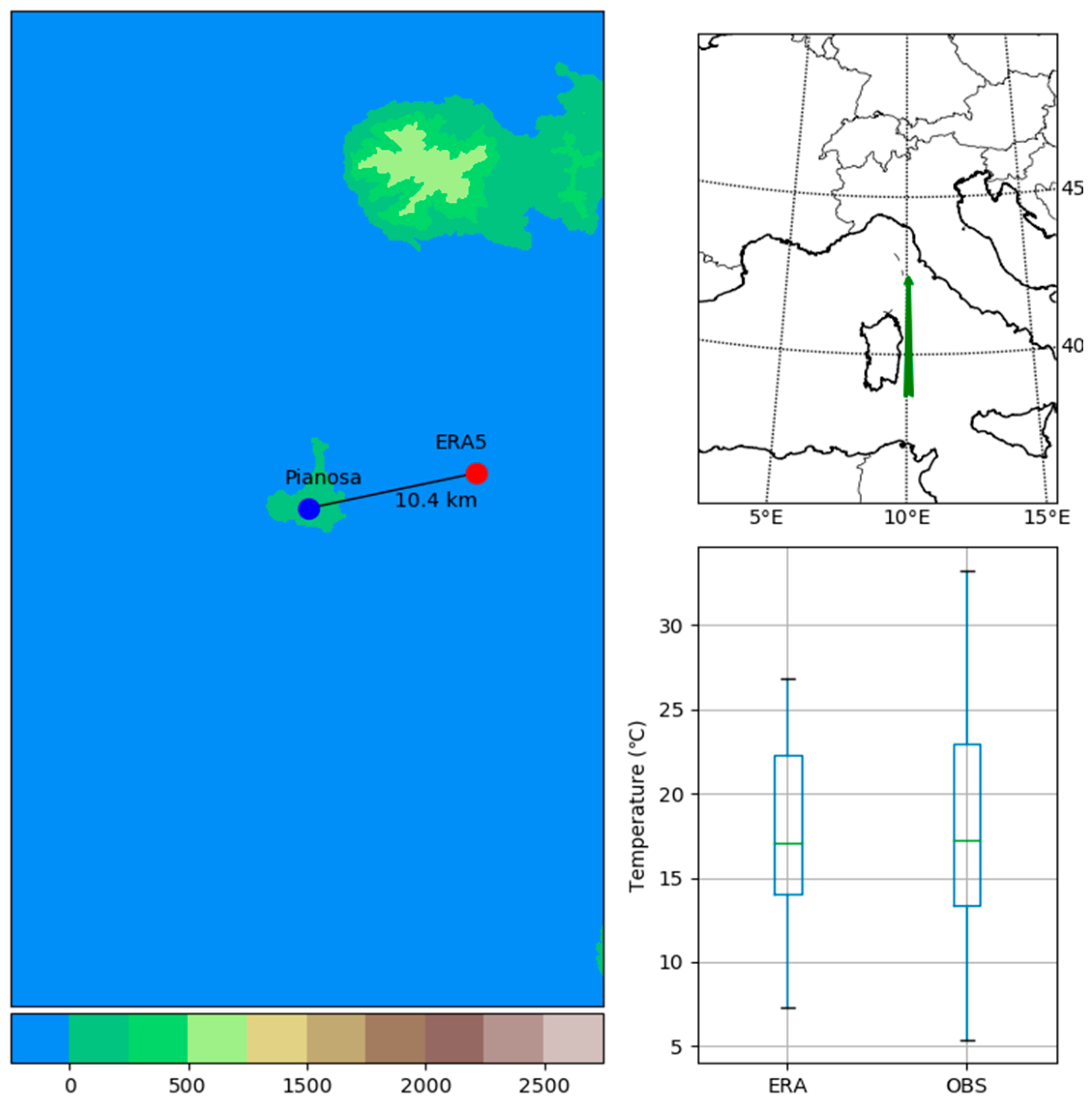
- Islands due to the coupling of sea surface processes and atmospheric processes and, in the case of small islands, their “visibility” on a 30 km resolution grid, which is highly questionable; and
- Desert oases, due to the position of these oases in tropical and subtropical areas where the meteorological measurement network is sparse.
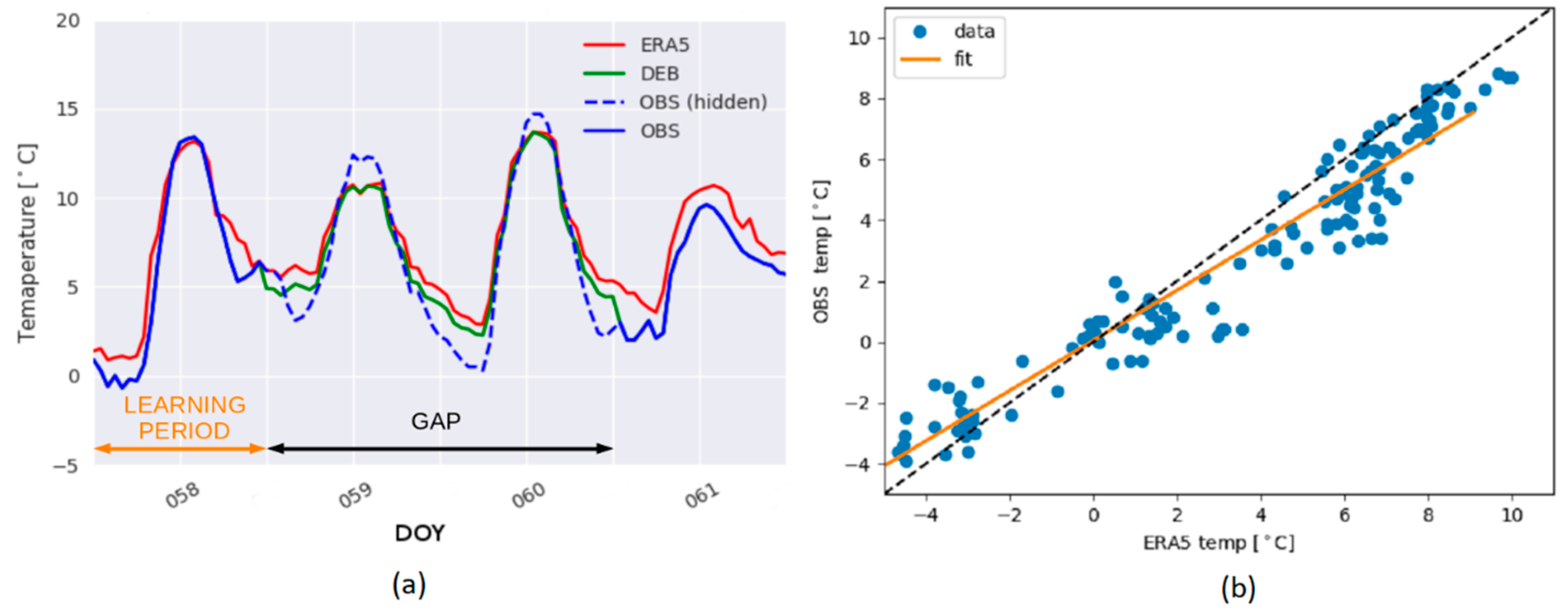
2.2. Gap Filling Method Description
- In the case of temperature data, due to the high autocorrelation of the time series, important information is contained within the time series before and after the gap [27]. Therefore, a portion of the time series that is not missing is used for the bias correction of ERA5 data;
- It is important to limit the amount of data used for the gap filling method (learning period) to avoid seasonal changes in temperature data; however, it is also important to use enough data to be able to exploit the high autocorrelation in the time series. The determination coefficient R2 was used to validate that enough data was present in the fitting process;
- Diurnal temperature biases [23] are recognized as a possible problem and new technique for filtering the learning data was applied to improve this methodology.
- To efficiently fill gaps in large datasets, a simple, fast, and reliable approach of linear regression was selected.
3. Results
3.1. Lowland Data Sets
3.2. Mountain Data Sets
3.3. Desert Data Sets
3.4. Island Data Sets
4. Discussion
5. Conclusions
Supplementary Materials
Author Contributions
Funding
Acknowledgments
Conflicts of Interest
Appendix A

| Pearson r | p Value | |||||||
|---|---|---|---|---|---|---|---|---|
| Min | Mean | Median | Max | Min | Mean | Median | Max | |
| Kikinda | 0.896 | 0.950 | 0.955 | 0.979 | 9.18 × 10−77 | 2.24 × 10−40 | 1.31 × 10−55 | 2.85 × 10−38 |
| Bahariya | 0.730 | 0.904 | 0.914 | 0.966 | 7.02 × 10−63 | 1.52 × 10⁻¹² | 1.72 × 10−38 | 1.83 × 10⁻¹⁰ |
| Gumpenstein | 0.762 | 0.889 | 0.894 | 0.957 | 4.01 × 10−36 | 7.66 × 10⁻¹⁰ | 8.25 × 10⁻²⁵ | 1.07 × 10⁻⁷ |
| Montecristo | 0.707 | 0.834 | 0.846 | 0.912 | 9.93 × 10⁻²⁸ | 5.80 × 10⁻¹⁰ | 3.75 × 10⁻¹⁸ | 3.49 × 10⁻⁸ |
| Pianosa | 0.545 | 0.760 | 0.747 | 0.939 | 5.69 × 10−36 | 0.002 | 1.83 × 10⁻⁹ | 0.029 |
| Input Quantity | Description | Location | Input Estimate | Standard Uncertainty | Pearson r | Measurement Unit | Type of Evaluation |
|---|---|---|---|---|---|---|---|
| M | Measured two-meter temperature | Kikinda | 17.2 | 5.2 | °C | A | |
| Gumpenstein | 12.8 | 4.4 | °C | A | |||
| Bahariya | 27.2 | 5.5 | °C | A | |||
| Montecristo | 21.3 | 1.9 | °C | A | |||
| Pianosa | 22.0 | 2.4 | °C | A | |||
| Predicted two-meter temperature (ERA5 reanalysis) | Kikinda | 17.6 | 4.4 | 0.966 | °C | A | |
| Gumpenstein | 8.4 | 4.3 | 0.849 | °C | A | ||
| Bahariya | 26.4 | 5.1 | 0.940 | °C | A | ||
| Montecristo | 21.3 | 1.1 | 0.753 | °C | A | ||
| Pianosa | 21.3 | 1.1 | 0.562 | °C | A | ||
| Predicted two-meter temperature (DEBIAS) | Kikinda | 17.2 | 5.1 | 0.969 | °C | A | |
| Gumpenstein | 13.3 | 4.2 | 0.905 | °C | A | ||
| Bahariya | 27.1 | 5.4 | 0.961 | °C | A | ||
| Montecristo | 21.6 | 1.6 | 0.854 | °C | A | ||
| Pianosa | 22.3 | 2.1 | 0.862 | °C | A |
Appendix B


Appendix C


References
- Eischeid, J.K.; Pasteris, P.A.; Diaz, H.F.; Plantico, M.S.; Lott, N.J. Creating a serially complete, national daily time series of temperature and precipitation for the western United States. J. Appl. Meteorol. 2000, 39, 1580–1591. [Google Scholar] [CrossRef]
- Henn, B.; Raleigh, M.S.; Fisher, A.; Lundquist, J.D. A comparison of methods for filling gaps in hourly near-surface air temperature data. J. Hydrometeorol. 2013, 14, 929–945. [Google Scholar] [CrossRef]
- Vuichard, N.; Papale, D. Filling the gaps in meteorological continuous data measured at FLUXNET sites with ERA-Interim reanalysis. Earth Syst. Sci. Data 2015, 7, 157–171. [Google Scholar] [CrossRef]
- Daly, S.F.; Davis, R.; Ochs, E.; Pangburn, T. An approach to spatially distributed snow modelling of the Sacramento and San Joaquin basins, California. Hydrol. Process. 2000, 14, 3257–3271. [Google Scholar] [CrossRef]
- Daly, C.; Gibson, W.P.; Taylor, G.H.; Johnson, G.L.; Pasteris, P. A knowledge-based approach to the statistical mapping of climate. Clim. Res. 2002, 22, 99–113. [Google Scholar] [CrossRef]
- Tobin, C.; Nicotina, L.; Parlange, M.B.; Berne, A.; Rinaldo, A. Improved interpolation of meteorological forcings for hydrologic applications in a Swiss Alpine region. J. Hydrol. 2011, 401, 77–89. [Google Scholar] [CrossRef]
- Garen, D.C.; Johnson, G.L.; Hanson, C.L. Mean Areal Precipitation for daily hydrologic modeling in mountainous regions. JAWRA J. Am. Water Resour. Assoc. 1994, 30, 481–491. [Google Scholar] [CrossRef]
- Hartkamp, A.D.; De Beurs, K.; Stein, A.; White, J.W. Interpolation Techniques for Climate Variables; Cimmyt: Mexico City, Mexico, 1999. [Google Scholar]
- Stahl, K.; Moore, R.D.; Floyer, J.A.; Asplin, M.G.; McKendry, I.G. Comparison of approaches for spatial interpolation of daily air temperature in a large region with complex topography and highly variable station density. Agric. For. Meteorol. 2006, 139, 224–236. [Google Scholar] [CrossRef]
- Pape, R.; Wundram, D.; Löffler, J. Modelling near-surface temperature conditions in high mountain environments: An appraisal. Clim. Res. 2009, 39, 99–109. [Google Scholar] [CrossRef]
- Minder, J.R.; Mote, P.W.; Lundquist, J.D. Surface temperature lapse rates over complex terrain: Lessons from the Cascade Mountains. J. Geophys. Res. Atmos. 2010, 115. [Google Scholar] [CrossRef]
- Rolland, C. Spatial and seasonal variations of air temperature lapse rates in Alpine regions. J. Clim. 2003, 16, 1032–1046. [Google Scholar] [CrossRef]
- Dodson, R.; Marks, D. Daily air temperature interpolated at high spatial resolution over a large mountainous region. Clim. Res. 1997, 8, 1–20. [Google Scholar] [CrossRef]
- Claridge, D.E.; Chen, H. Missing data estimation for 1–6 h gaps in energy use and weather data using different statistical methods. Int. J. Energy Res. 2006, 30, 1075–1091. [Google Scholar] [CrossRef]
- Liston, G.E.; Elder, K. A meteorological distribution system for high-resolution terrestrial modeling (MicroMet). J. Hydrometeorol. 2006, 7, 217–234. [Google Scholar] [CrossRef]
- Von Storch, H.; Zwiers, F.W.; Livezey, R.E. Statistical analysis in climate research. Nature 2000, 404, 544. [Google Scholar]
- Beckers, J.-M.; Rixen, M. EOF calculations and data filling from incomplete oceanographic datasets. J. Atmos. Ocean. Technol. 2003, 20, 1839–1856. [Google Scholar] [CrossRef]
- Blyth, E.; Gash, J.; Lloyd, A.; Pryor, M.; Weedon, G.P.; Shuttleworth, J. Evaluating the JULES land surface model energy fluxes using FLUXNET data. J. Hydrometeorol. 2010, 11, 509–519. [Google Scholar] [CrossRef]
- Stöckli, R.; Lawrence, D.M.; Niu, G.-Y.; Oleson, K.W.; Thornton, P.E.; Yang, Z.-L.; Bonan, G.B.; Denning, A.S.; Running, S.W. Use of FLUXNET in the Community Land Model development. J. Geophys. Res. Biogeosci. 2008, 113. [Google Scholar] [CrossRef]
- Papale, D. Data gap filling. In Eddy Covariance; Springer: Berlin, Germany, 2012; pp. 159–172. [Google Scholar]
- Puri, K. Numerical weather prediction in the tropics. J. Meteorol. Soc. Jpn. Ser II 1986, 64, 605–631. [Google Scholar] [CrossRef]
- Sandu, I.; Bechtold, P.; Beljaars, A.; Bozzo, A.; Pithan, F.; Shepherd, T.G.; Zadra, A. Impacts of parameterized orographic drag on the Northern Hemisphere winter circulation. J. Adv. Model. Earth Syst. 2016, 8, 196–211. [Google Scholar] [CrossRef]
- Haiden, T.; Sandu, I.; Balsamo, G.; Arduini, G.; Beljaar, A. Addressing Biases in Near-Surface Forecasts; ECMWF Newsletter; European Centre for Medium-Range Weather Forecasts: Shinfield Park, Reading, UK, 2018; p. 157. [Google Scholar]
- Lim, Y.-K.; Cai, M.; Kalnay, E.; Zhou, L. Observational evidence of sensitivity of surface climate changes to land types and urbanization. Geophys. Res. Lett. 2005, 32. [Google Scholar] [CrossRef]
- ERA5 Data Documentation—Copernicus Knowledge Base—ECMWF Confluence Wiki. Available online: https://confluence.ecmwf.int//display/CKB/ERA5+data+documentation (accessed on 5 November 2018).
- LaMMA Consortium. Available online: http://www.lamma.rete.toscana.it/ (accessed on 24 November 2018).
- Raible, C.C.; Bischof, G.; Fraedrich, K.; Kirk, E. Statistical single-station short-term forecasting of temperature and probability of precipitation: Area interpolation and NWP combination. Weather Forecast. 1999, 14, 203–214. [Google Scholar] [CrossRef]
- FDA U. NIST: Multi-Agency Radiological Laboratory Analytical Protocols Manual (MARLAP); FDA, USGS, NUREG-1576. EPA 402-B-04-001C, NTIS PB2004-105421; FDA: Alexandria, VA, USA, 2004. [Google Scholar]
- D’Agostino, R.B. An omnibus test of normality for moderate and large size samples. Biometrika 1971, 58, 341–348. [Google Scholar] [CrossRef]
- D’Agostino, R.B.; Pearson, E.S. Tests for departure from normality. Empirical results for the distributions of b 2 and√ b. Biometrika 1973, 60, 613–622. [Google Scholar] [CrossRef]
- Pavlovič, F.; Nastran, J.; Nedeljković, D. Determining the 95% Confidence Interval of Arbitrary Non-Gaussian probability distributions. Available online: http://www.imeko2009.it.pt/Papers/FP_81.pdf (accessed on 13 October 2018).
- Dumas, M.D. Changes in temperature and temperature gradients in the French Northern Alps during the last century. Theor. Appl. Climatol. 2013, 111, 223–233. [Google Scholar] [CrossRef]
- Evans, J.D. Straightforward Statistics for the Behavioral Sciences; Brooks/Cole Publishing Company: Pacific Grove, CA, USA, 1996; ISBN 978-0-534-23100-2. [Google Scholar]
- Cao, H.X.; Mitchell, J.F.B.; Lavery, J.R. Simulated Diurnal Range and Variability of Surface Temperature in a Global Climate Model for Present and Doubled CO2 Climates. J. Clim. 1992, 5, 920–943. [Google Scholar] [CrossRef]
- Decker, M.; Brunke, M.A.; Wang, Z.; Sakaguchi, K.; Zeng, X.; Bosilovich, M.G. Evaluation of the reanalysis products from GSFC, NCEP, and ECMWF using flux tower observations. J. Clim. 2012, 25, 1916–1944. [Google Scholar] [CrossRef]
- Chen, Z. A Serially Complete, U.S. Dataset of Temperature and Precipitation for Decision Support Systems. J. Environ. Inform. 2006, 8, 86–99. [Google Scholar] [CrossRef]


| Location | Time Series | Landscape | Position | ERA5 | ||||
|---|---|---|---|---|---|---|---|---|
| Latitude (°) | Longitude (°) | Altitude (m) | Latitude (°) | Longitude (°) | Altitude (m) | |||
| Kikinda | 2014–2017 | Lowland | 45.87 | 20.46 | 82 | 45.9 | 20.4 | 75 |
| Gumpenstein | 2014–2017 | Mountains | 47.49 | 14.09 | 700 | 47.4 | 14.1 | 1080 |
| Bahariya | 2017 | Desert | 28.41 | 28.93 | 99 | 28.4 | 28.9 | 97 |
| Montecristo | 2016 | Island | 42.34 | 10.31 | 645 | 42.3 | 10.2 | * |
| Pianosa | 2016 | Island | 42.58 | 10.08 | 29 | 42.6 | 10.2 | * |
| Mean B | Mean U(B) | Mean RMSE | ||||
|---|---|---|---|---|---|---|
| ERA5 | DEB | ERA5 | DEB | ERA5 | DEB | |
| Kikinda | 0.387 | −0.027 | 6.56 | 5.61 | 1.563 | 1.321 |
| Bahariya | −0.723 | −0.033 | 8.39 | 6.67 | 2.046 | 1.536 |
| Gumpenstein | −4.385 | 0.556 | 10.18 | 7.37 | 4.969 | 1.877 |
| Montecristo | −0.009 | 0.284 | 5.58 | 4.27 | 1.367 | 1.079 |
| Pianosa | −0.769 | 0.222 | 8.69 | 5.32 | 2.158 | 1.260 |
| Location | Bahariya (°C) | Gumpenstein (°C) | Kikinda (°C) | Montecristo (°C) | Pianosa (°C) |
|---|---|---|---|---|---|
| max(|RMSEDEB-RMSEERA5|) for hourly data | 1.81 | 6.34 | 0.87 | 0.95 | 2.12 |
| max(|RMSEDEB-RMSEERA5|) for daily average | 1.31 | 7.32 | 1.03 | 1.08 | 1.63 |
| max(|RMSEDEB|) for hourly data | 2.54 | 4.19 | 2.21 | 2.18 | 2.31 |
| max(|RMSEDEB|) for daily average | 1.82 | 4.02 | 1.69 | 2.06 | 1.98 |
© 2019 by the authors. Licensee MDPI, Basel, Switzerland. This article is an open access article distributed under the terms and conditions of the Creative Commons Attribution (CC BY) license (http://creativecommons.org/licenses/by/4.0/).
Share and Cite
Lompar, M.; Lalić, B.; Dekić, L.; Petrić, M. Filling Gaps in Hourly Air Temperature Data Using Debiased ERA5 Data. Atmosphere 2019, 10, 13. https://doi.org/10.3390/atmos10010013
Lompar M, Lalić B, Dekić L, Petrić M. Filling Gaps in Hourly Air Temperature Data Using Debiased ERA5 Data. Atmosphere. 2019; 10(1):13. https://doi.org/10.3390/atmos10010013
Chicago/Turabian StyleLompar, Miloš, Branislava Lalić, Ljiljana Dekić, and Mina Petrić. 2019. "Filling Gaps in Hourly Air Temperature Data Using Debiased ERA5 Data" Atmosphere 10, no. 1: 13. https://doi.org/10.3390/atmos10010013
APA StyleLompar, M., Lalić, B., Dekić, L., & Petrić, M. (2019). Filling Gaps in Hourly Air Temperature Data Using Debiased ERA5 Data. Atmosphere, 10(1), 13. https://doi.org/10.3390/atmos10010013