Habitat Fragmentation Reduces Genetic Diversity and Connectivity of the Mexican Spotted Owl: A Simulation Study Using Empirical Resistance Models


Abstract
1. Introduction
2. Materials and Methods
2.1. Study Species
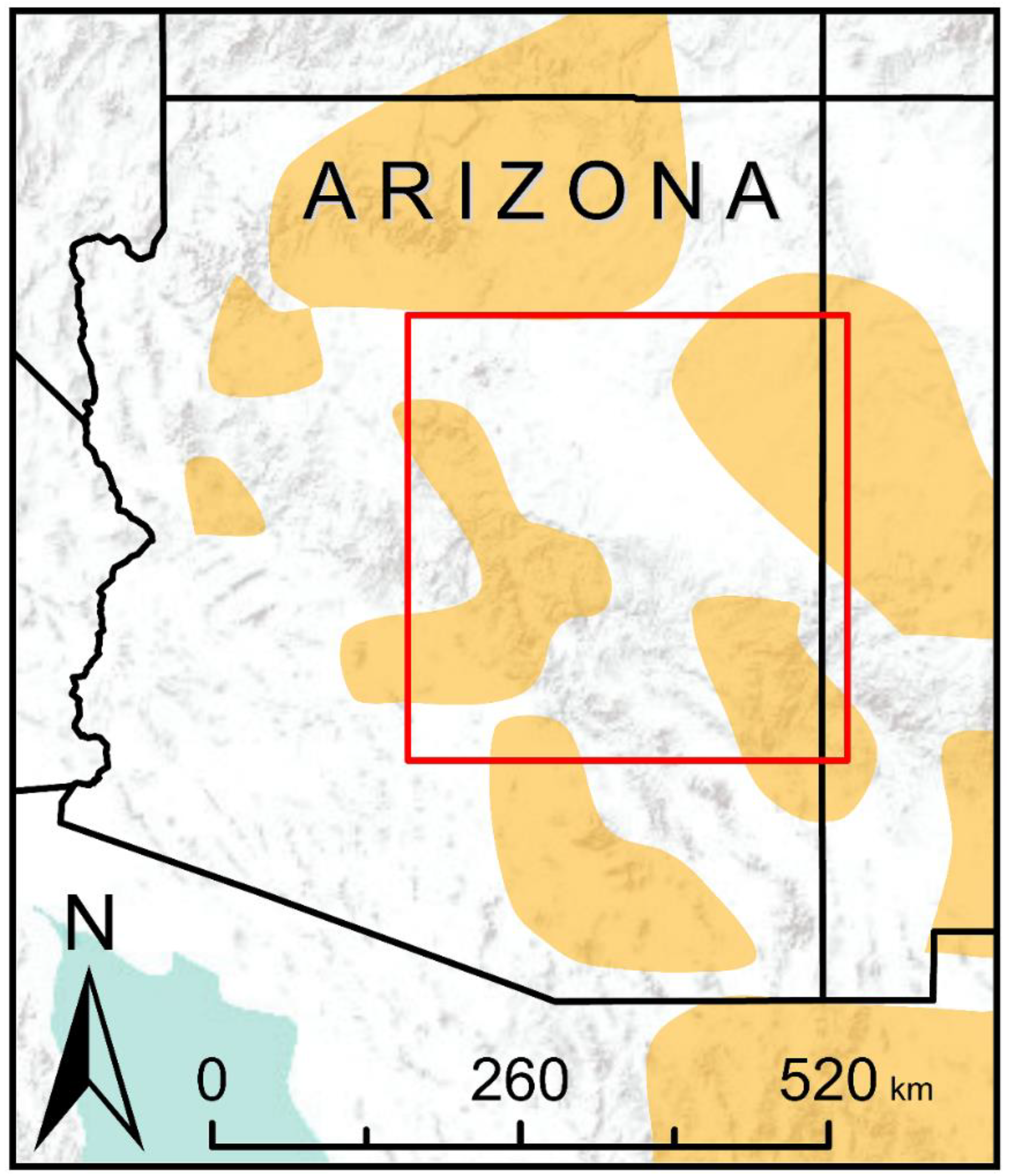
2.2. Study Area
2.3. Resistance Models
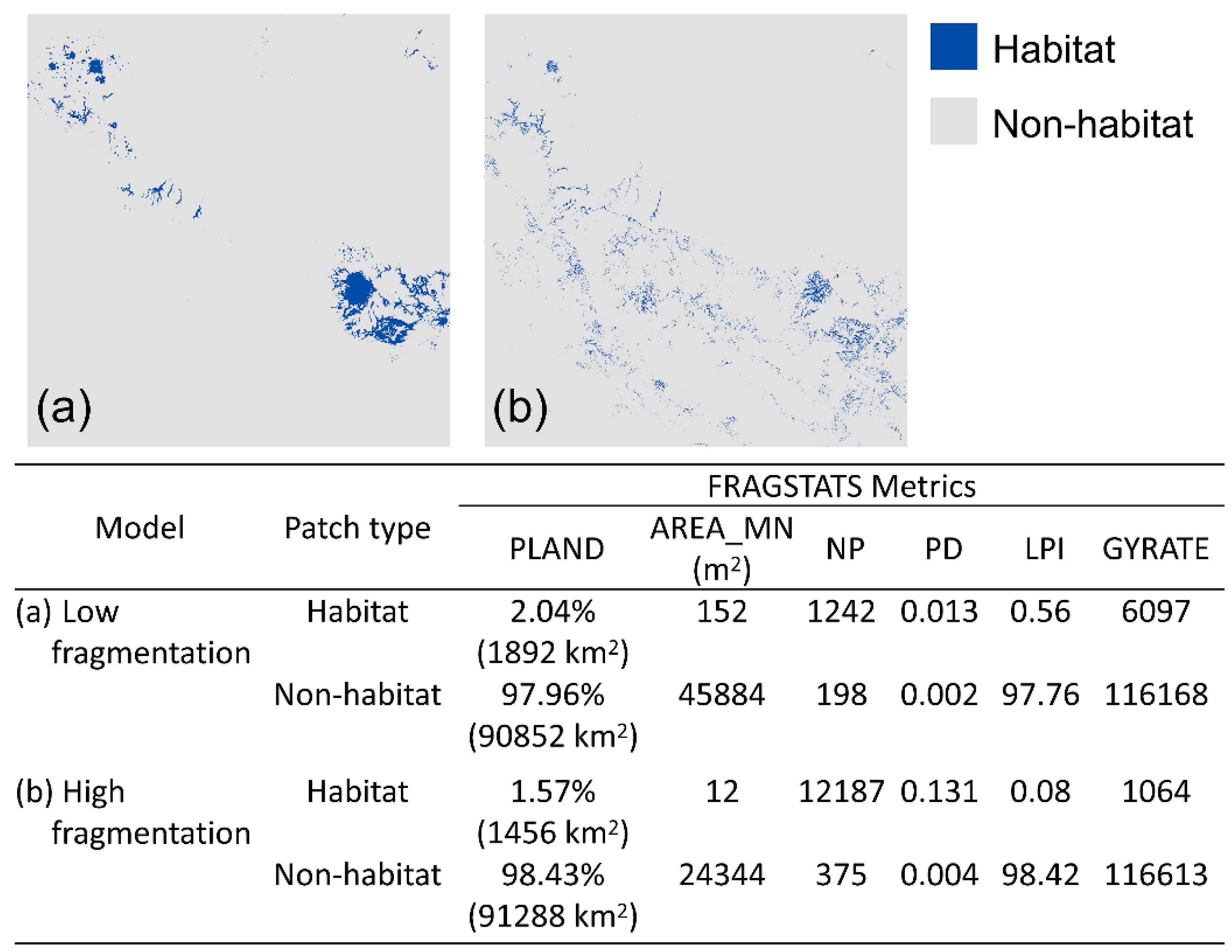
2.4. Fragmentation Analysis
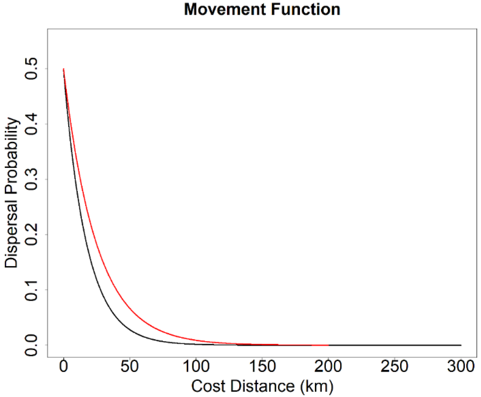
2.5. Landscape Genetics Simulation
- Isolation-by-distance (IBD): This hypothesis serves as a null model and assumes that species movement decisions are affected purely by geographic distance, and genetic exchange occurs more frequently between proximate individuals than distant individuals.
- Isolation-by-resistance (IBR): This hypothesis posits that species movement decisions and resulting gene flow are influenced by landscape features and patterns associated with resource selection.
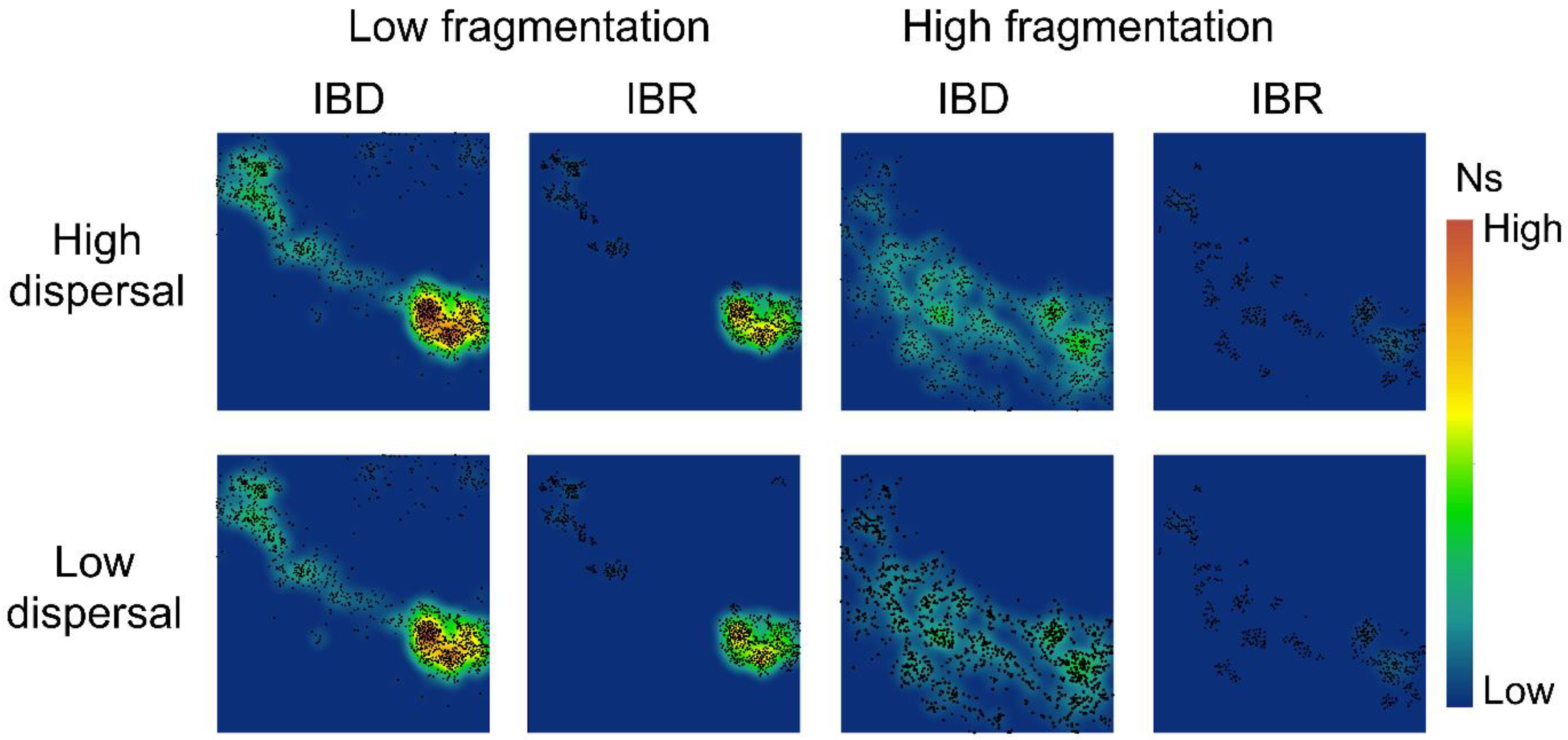
2.6. Spatial Population Patterns
2.7. Genetic Diversity
2.8. Resistance Cost Distance and Genetic Distance
2.9. Genetic Diversity and Landscape Connectivity Relationships
3. Results
3.1. Fragmentation Analysis
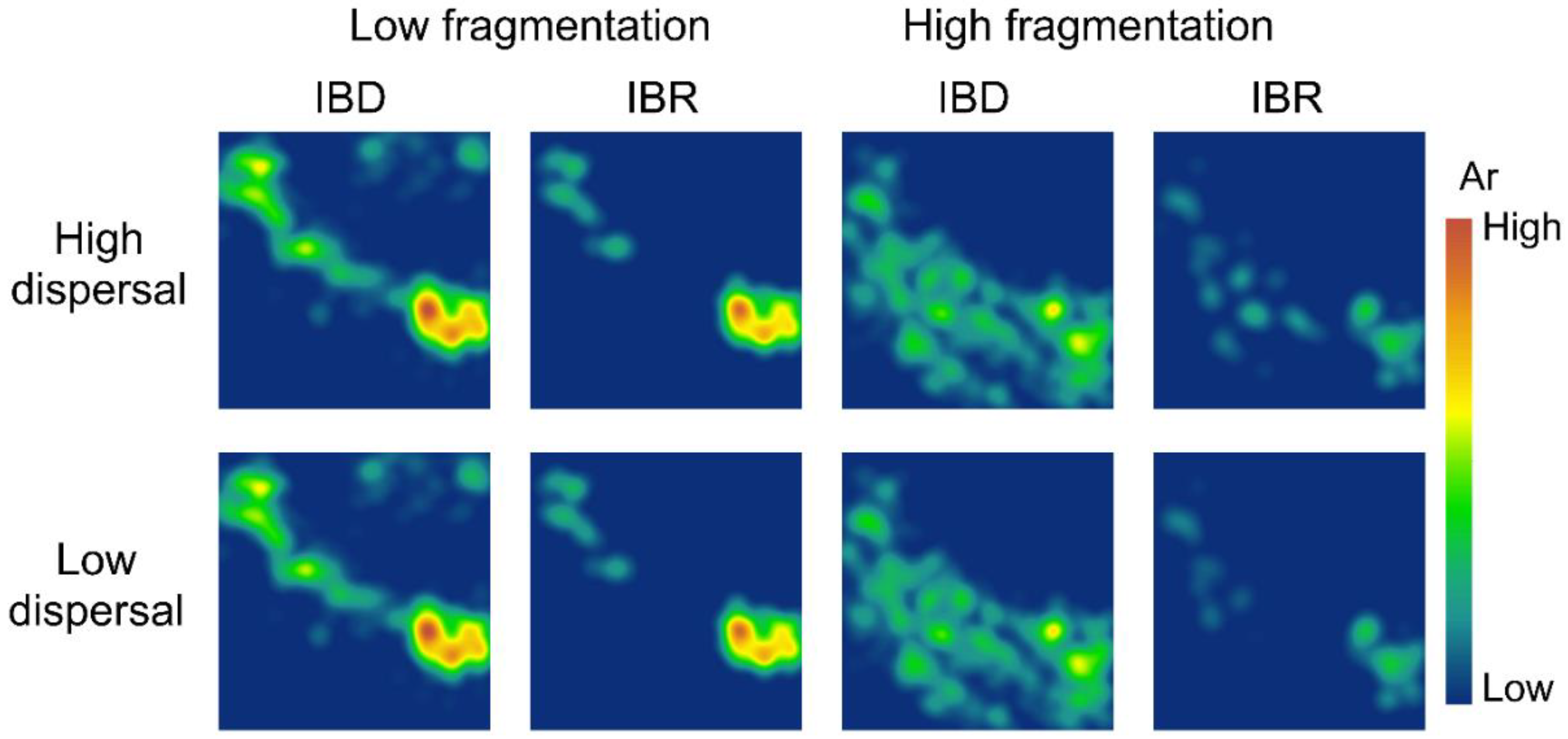
3.2. Spatial Patterns of Effective Population Size and Genetic Diversity
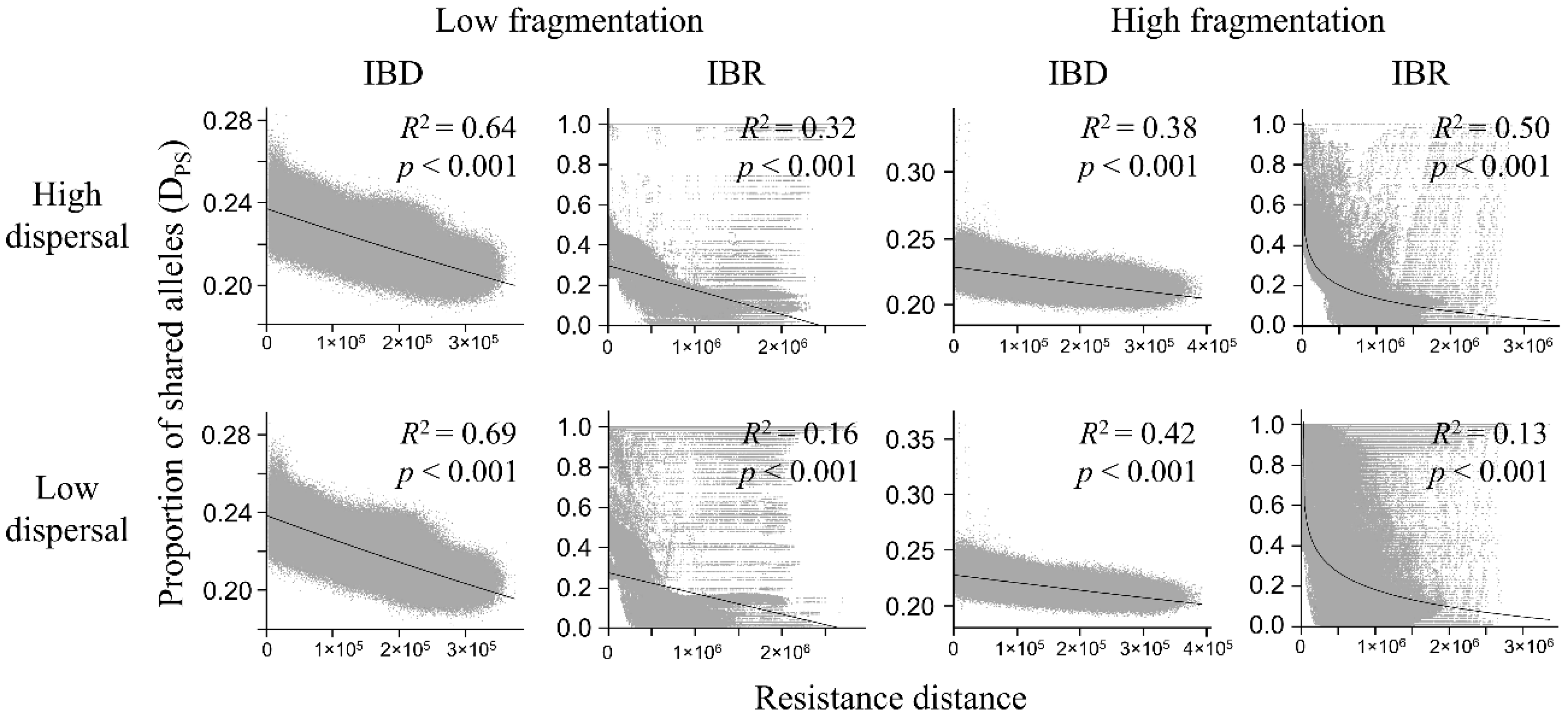
3.3. Genetic Distance Increased with Resistance Distance
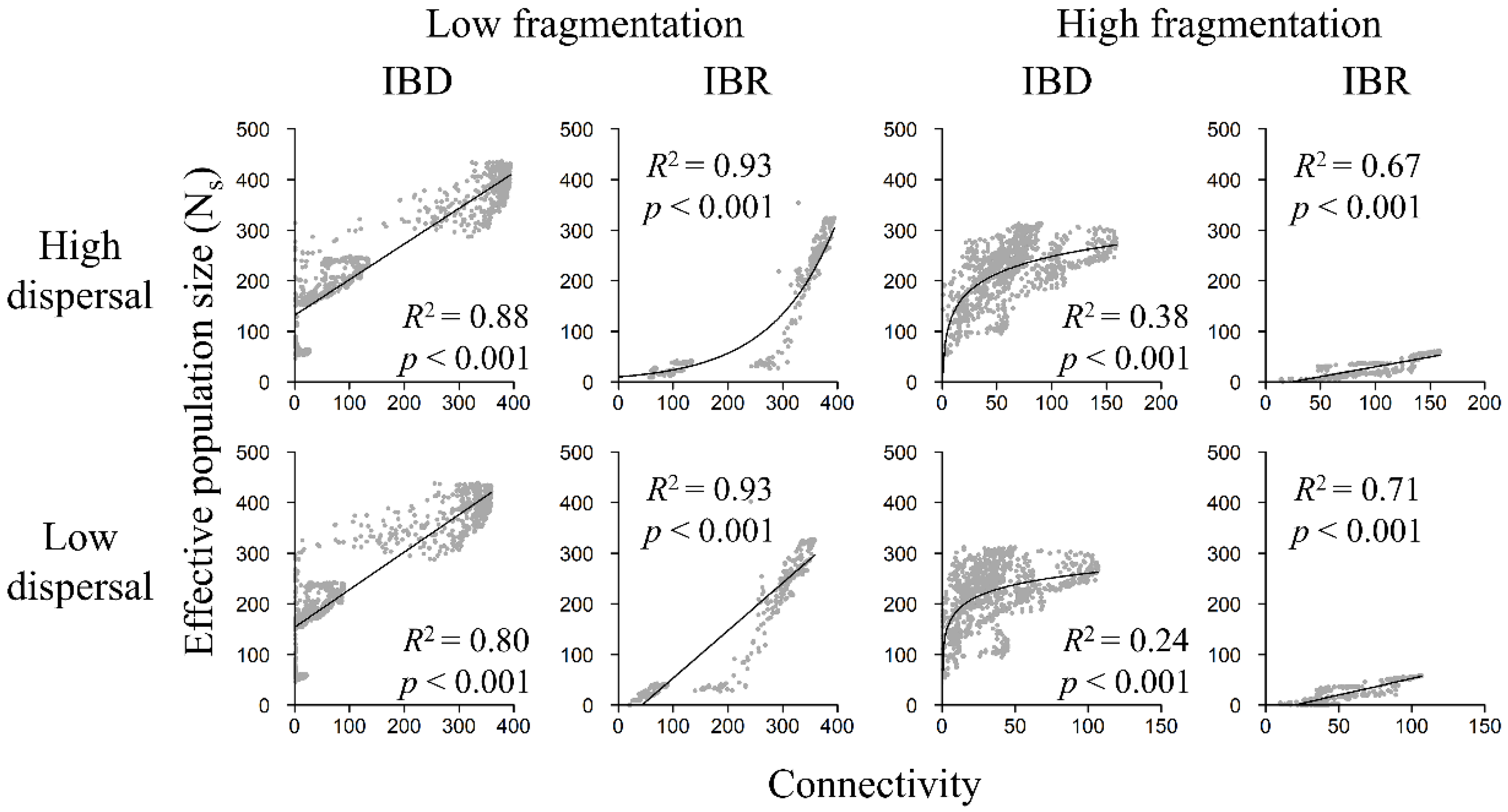
3.4. Population Size and Landscape Connectivity Relationships
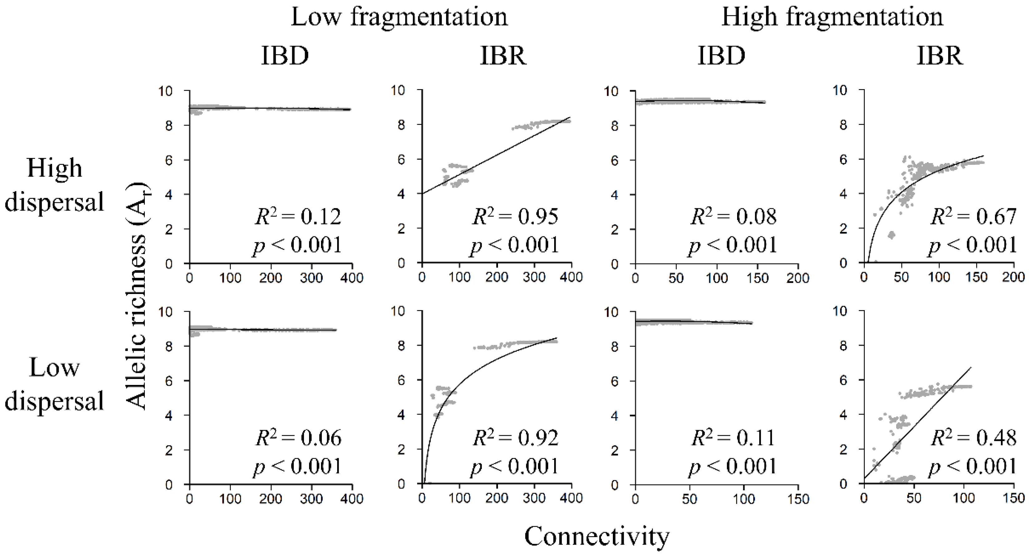
3.5. Genetic Diversity and Landscape Connectivity Relationships
4. Discussion
4.1. Connectivity Facilitated Gene Flow
4.2. Linear, Logarithmic, and Exponential Relationships
4.3. Aggregated and Concentrated vs. Fragmented and Widespread Landscapes
4.4. Comparison with Empirical Data on Genetic Structure
5. Conclusions
Supplementary Materials
Author Contributions
Funding
Acknowledgments
Conflicts of Interest
References
- Fahrig, L. Effects of habitat fragmentation on biodiversity. Annu. Rev. Ecol. Evol. Syst. 2003, 34, 487–515. [Google Scholar] [CrossRef]
- Pimm, S.L.; Jenkins, C.N.; Abell, R.; Brooks, T.M.; Gittleman, J.L.; Joppa, L.N.; Raven, P.H.; Roberts, C.M.; Sexton, J.O. The biodiversity of species and their rates of extinction, distribution, and protection. Science 2014, 344, 1246752. [Google Scholar] [CrossRef] [PubMed]
- Newbold, T.; Hudson, L.N.; Hill, S.L.; Contu, S.; Lysenko, I.; Senior, R.A.; Börger, L.; Bennett, D.J.; Choimes, A.; Collen, B.; et al. Global effects of land use on local terrestrial biodiversity. Nature 2015, 520, 45–50. [Google Scholar] [CrossRef] [PubMed]
- IUCN Species Survival Commission. 2015 Annual Report of the Species Survival Commission and the Global Species Programme; International Union for Conservation of Nature: Gland, Switzerland, 2015. [Google Scholar]
- Cushman, S.A. Effects of habitat loss and fragmentation on amphibians: A review and prospectus. Biol. Conserv. 2006, 128, 231–240. [Google Scholar] [CrossRef]
- Leidner, A.K.; Haddad, N.M. Combining measures of dispersal to identify conservation strategies in fragmented landscapes. Conserv. Biol. 2011, 25, 1022–1031. [Google Scholar] [CrossRef] [PubMed]
- Frankham, R. Genetics and extinction. Biol. Conserv. 2005, 126, 131–140. [Google Scholar] [CrossRef]
- Honnay, O.; Jacquemyn, H. Susceptibility of common and rare plant species to the genetic consequences of habitat fragmentation. Conserv. Biol. 2007, 21, 823–831. [Google Scholar] [CrossRef] [PubMed]
- Aguilar, R.; Quesada, M.; Ashworth, L.; Herrerias–Diego, Y.; Lobo, J. Genetic consequences of habitat fragmentation in plant populations: Susceptible signals in plant traits and methodological approaches. Mol. Ecol. 2008, 17, 5177–5188. [Google Scholar] [CrossRef] [PubMed]
- Mech, S.; Hallett, J.G. Evaluating the effectiveness of corridors: A genetic approach. Conserv. Biol. 2001, 15, 467–474. [Google Scholar] [CrossRef]
- Gilbert–Norton, L.; Wilson, R.; Stevens, J.R.; Beard, K.H. A meta–analytic review of corridor effectiveness. Conserv. Biol. 2010, 24, 660–668. [Google Scholar] [CrossRef] [PubMed]
- Manel, S.; Schwartz, M.K.; Luikart, G.; Taberlet, P. Landscape genetics: Combining landscape ecology and population genetics. Trends Ecol. Evol. 2003, 18, 189–197. [Google Scholar] [CrossRef]
- Balkenhol, N.; Cushman, S.A.; Storfer, A.; Waits, L.P. Introduction to landscape genetics—concepts, methods, applications. In Landscape Genetics: Concepts, Methods, Applications; Balkenhol, N., Cushman, S.A., Storfer, A.T., Waits, L.P., Eds.; John Wiley and Sons: Chichester, UK, 2016; pp. 1–7. ISBN 978-1-118-52529-6. [Google Scholar]
- Holderegger, R.; Wagner, H.H. A brief guide to landscape genetics. Landsc. Ecol. 2006, 21, 793–796. [Google Scholar] [CrossRef]
- Storfer, A.; Murphy, M.A.; Evans, J.S.; Goldberg, C.S.; Robinson, S.; Spear, S.F.; Dezzani, R.; Delmelle, E.; Vierling, L.; Waits, L.P. Putting the ‘landscape’ in landscape genetics. Heredity 2007, 98, 128–142. [Google Scholar] [CrossRef] [PubMed]
- Balkenhol, N.; Waits, L.P.; Dezzani, R.J. Statistical approaches in landscape genetics: An evaluation of methods for linking landscape and genetic data. Ecography 2009, 32, 818–830. [Google Scholar] [CrossRef]
- Manel, S.; Joost, S.; Epperson, B.K.; Holderegger, R.; Storfer, A.; Rosenberg, M.S.; Scribner, K.T.; Bonin, A.; Fortin, M. Perspectives on the use of landscape genetics to detect genetic adaptive variation in the field. Mol. Ecol. 2010, 19, 3760–3772. [Google Scholar] [CrossRef] [PubMed]
- Landguth, E.L.; Holden, Z.A.; Mahalovich, M.F.; Cushman, S.A. Using landscape genetics simulations for planting blister rust resistant whitebark pine in the US Northern Rocky Mountains. Front. Genet. 2017, 8, 9. [Google Scholar] [CrossRef] [PubMed]
- Thatte, P.; Joshi, A.; Vaidyanathan, S.; Landguth, E.; Ramakrishnan, U. Maintaining tiger connectivity and minimizing extinction into the next century: Insights from landscape genetics and spatially-explicit simulations. Biol. Conserv. 2018, 218, 181–191. [Google Scholar] [CrossRef]
- Wasserman, T.N.; Cushman, S.A.; Shirk, A.S.; Landguth, E.L.; Littell, J.S. Simulating the effects of climate change on population connectivity of American marten (Martes americana) in the northern Rocky Mountains, USA. Landsc. Ecol. 2012, 27, 211–225. [Google Scholar] [CrossRef]
- Wasserman, T.N.; Cushman, S.A.; Littell, J.S.; Shirk, A.J.; Landguth, E.L. Population connectivity and genetic diversity of American marten (Martes americana) in the United States northern Rocky Mountains in a climate change context. Conserv. Genet. 2013, 14, 529–541. [Google Scholar] [CrossRef]
- Cushman, S.A.; McKelvey, K.S.; Schwartz, M.K. Use of empirically derived source-destination models to map regional conservation corridors. Conserv. Biol. 2009, 23, 368–376. [Google Scholar] [CrossRef] [PubMed]
- Brodie, J.F.; Giordano, A.J.; Dickson, B.G.; Hebblewhite, M.; Bernard, H.; Mohd–Azlan, J.; Anderson, J.; Ambu, L. Evaluating multispecies landscape connectivity in a threatened tropical mammal community. Conserv. Biol. 2015, 29, 122–132. [Google Scholar] [CrossRef] [PubMed]
- Zeller, K.A.; Vickers, T.W.; Ernest, H.B.; Boyce, W.M. Multi–level, multi–scale resource selection functions and resistance surfaces for conservation planning: Pumas as a case study. PLoS ONE 2017, 12, e0179570. [Google Scholar] [CrossRef] [PubMed]
- Landguth, E.L.; Muhlfeld, C.C.; Waples, R.S.; Jones, L.; Lowe, W.H.; Whited, D.; Lucotch, J.; Neville, H.; Luikart, G. Combining demographic and genetic factors to assess population vulnerability in stream species. Ecol. Appl. 2014, 24, 1505–1524. [Google Scholar] [CrossRef] [PubMed]
- Van Strien, M.J.; Keller, D.; Holderegger, R.; Ghazoul, J.; Kienast, F.; Bolliger, J. Landscape genetics as a tool for conservation planning: Predicting the effects of landscape change on gene flow. Ecol. Appl. 2014, 24, 327–339. [Google Scholar] [CrossRef] [PubMed]
- Bothwell, H.M.; Cushman, S.A.; Woolbright, S.A.; Hersch-Green, E.I.; Evans, L.M.; Whitham, T.G.; Allan, G.J. Conserving threatened riparian ecosystems in the American West: Precipitation gradients and river networks drive genetic connectivity and diversity in a foundation riparian tree (Populus angustifolia). Mol. Ecol. 2017, 26, 5114–5132. [Google Scholar] [CrossRef] [PubMed]
- Cushman, S.A.; McKelvey, K.S.; Hayden, J.; Schwartz, M.K. Gene flow in complex landscapes: Testing multiple hypotheses with causal modeling. Am. Nat. 2006, 168, 486–499. [Google Scholar] [CrossRef] [PubMed]
- McRae, B.H. Isolation by resistance. Evolution 2006, 60, 1551–1561. [Google Scholar] [CrossRef] [PubMed]
- Spear, S.F.; Balkenhol, N.; Fortin, M.; McRae, B.H.; Scribner, K. Use of resistance surfaces for landscape genetic studies: Considerations for parameterization and analysis. Mol. Ecol. 2010, 19, 3576–3591. [Google Scholar] [CrossRef] [PubMed]
- Cushman, S.A.; Shirk, A.J.; Landguth, E.L. Landscape genetics and limiting factors. Conserv. Genet. 2013, 14, 263–274. [Google Scholar] [CrossRef]
- Kozakiewicz, C.P.; Carver, S.; Burridge, C.P. Under–representation of avian studies in landscape genetics. Int. J. Avian Sci. 2018, 160, 1–12. [Google Scholar] [CrossRef]
- Bonnet, X.; Shine, R.; Lourdais, O. Taxonomic chauvinism. Trends Ecol. Evol. 2002, 17, 1–3. [Google Scholar] [CrossRef]
- Clark, J.A.; May, R.M. Taxonomic bias in conservation research. Science 2002, 297, 191–192. [Google Scholar] [CrossRef] [PubMed]
- Pawar, S. Taxonomic chauvinism and the methodologically challenged. BioScience 2003, 53, 861–864. [Google Scholar] [CrossRef]
- Seddon, P.J.; Soorae, P.S.; Launay, F. Taxonomic bias in reintroduction projects. Anim. Conserv. 2005, 8, 51–58. [Google Scholar] [CrossRef]
- Taborsky, M. Biased citation practice and taxonomic parochialism. Ethology 2009, 115, 105–111. [Google Scholar] [CrossRef]
- Stahlschmidt, Z.R. Taxonomic chauvinism revisited: Insight from parental care research. PLoS ONE 2011, 6, e24192. [Google Scholar] [CrossRef] [PubMed]
- Martínez–Cruz, B.; Godoy, J.A.; Negro, J.J. Population fragmentation leads to spatial and temporal genetic structure in the endangered Spanish imperial eagle. Mol. Ecol. 2007, 16, 477–486. [Google Scholar] [CrossRef] [PubMed]
- Peery, M.Z.; Hall, L.A.; Sellas, A.; Beissinger, S.R.; Moritz, C.; Berube, M.; Raphael, M.G.; Nelson, S.K.; Golightly, R.T.; McFarlane-Tranquilla, L.; et al. Genetic analyses of historic and modern marbled murrelets suggest decoupling of migration and gene flow after habitat fragmentation. Proc. Royal Soc. Lond. B Biol. Sci. 2010, 277, 697–706. [Google Scholar] [CrossRef] [PubMed]
- Edelaar, P.; Alonso, D.; Lagerveld, S.; Senar, J.C.; Bjorklund, M. Population differentiation and restricted gene flow in Spanish crossbills: Not isolation–by–distance but isolation–by–ecology. J. Evol. Biol. 2012, 25, 417–430. [Google Scholar] [CrossRef] [PubMed]
- U.S. Department of Interior. Final Recovery Plan for the Mexican Spotted Owl (Strix occidentalis lucida), First Revision; U.S. Fish and Wildlife Service: Albuquerque, NM, USA, 2012.
- Gutiérrez, R.J.; Seamans, M.E.; Peery, M.Z. Intermountain movement by Mexican spotted owls (Strix occidentalis lucida). Gt. Basin Nat. 1996, 56, 87–89. [Google Scholar]
- Ganey, J.L.; Block, W.M.; Dwyer, J.K.; Strohmeyer, B.E.; Jenness, J.S. Dispersal movements and survival rates of juvenile Mexican spotted owls in northern Arizona. Wilson Bull. 1998, 110, 206–217. [Google Scholar]
- Willey, D.W.; van Riper, C., III. First-year movements by juvenile Mexican spotted owls in the canyonlands of Utah. J. Raptor Res. 2000, 34, 1–7. [Google Scholar]
- Ganey, J.L.; Jenness, J.S. An Apparent Case of Long Distance Breeding Dispersal by a Mexican Spotted Owl in New Mexico; Research Note RMRS–RN–53WWW; U.S. Department of Agriculture, Forest Service, Rocky Mountain Research Station: Fort Collins, CO, USA, 2013.
- Wan, H.Y. Habitat, Connectivity, and Gene Flow of Mexican Spotted Owl in southwestern Forests. Ph.D. Dissertation, Northern Arizona University, Flagstaff, AZ, USA, 2018. [Google Scholar]
- Wan, H.Y.; Cushman, S.A.; Ganey, J.L. Improving habitat and connectivity model predictions with multi-scale resource selection functions from two geographic areas. Landsc. Ecol. 2018. under review. [Google Scholar]
- Ganey, J.L.; Balda, R.P. Distribution and habitat use of Mexican spotted owls in Arizona. Condor 1989, 91, 355–361. [Google Scholar] [CrossRef]
- Ganey, J.L.; Balda, R.P. Habitat selection by Mexican spotted owls in northern Arizona. Auk 1994, 111, 162–169. [Google Scholar] [CrossRef]
- Seamans, M.E.; Gutiérrez, R.J. Breeding habitat of the Mexican spotted owl in the Tularosa Mountains, New Mexico. Condor 1995, 97, 944–952. [Google Scholar] [CrossRef]
- Ganey, J.L.; Block, W.M.; Jenness, J.S.; Wilson, R.A. Mexican spotted owl home range and habitat use in pine–oak forest: Implications for forest management. For. Sci. 1999, 45, 127–135. [Google Scholar]
- Peery, M.Z.; Gutiérrez, R.J.; Seamans, M.E. Habitat composition and configuration around Mexican spotted owl nest and roost sites in the Tularosa Mountains, New Mexico. J. Wildl. Manag. 1999, 63, 36–43. [Google Scholar] [CrossRef]
- Willey, D.W.; van Riper, C., III. Home range characteristics of Mexican spotted owls in the Canyonlands of Utah. J. Raptor Res. 2007, 41, 10–15. [Google Scholar] [CrossRef]
- Timm, B.C.; McGarigal, K.; Cushman, S.A.; Ganey, J.L. Multi–scale Mexican spotted owl (Strix occidentalis lucida) nest/roost habitat selection in Arizona and a comparison with single–scale modeling results. Landsc. Ecol. 2016, 31, 1209–1225. [Google Scholar] [CrossRef]
- Wan, H.Y.; McGarigal, K.; Ganey, J.L.; Lauret, V.; Timm, B.C.; Cushman, S.A. Meta-replication reveals nonstationarity in multi-scale habitat selection of Mexican Spotted Owl. Condor 2017, 119, 641–658. [Google Scholar] [CrossRef]
- Seamans, M.E.; Gutiérrez, R.J.; May, C.A.; Peery, M.Z. Demography of two Mexican spotted owl populations. Conserv. Biol. 1999, 13, 744–754. [Google Scholar] [CrossRef]
- Stacey, P.B.; Peery, M.Z. Population trends of the Mexican spotted owl in west–central New Mexico. New Mex. Ornithol. Soc. Bull. 2002, 30, 42. [Google Scholar]
- U.S. Department of Interior. Endangered and threatened wildlife and plants; Final rule to list the Mexican Spotted Owl as a threatened species, U.S. Fish and Wildlife Service. Fed. Regist. 1993, 58, 14248–14271. [Google Scholar]
- Ganey, J.L.; Wan, H.Y.; Cushman, S.A.; Vojta, C.D. Conflicting perspectives on spotted owls, wildfire, and forest restoration. Fire Ecol. 2017, 13, 146–165. [Google Scholar] [CrossRef]
- Wan, H.Y.; Ganey, J.L.; Vojta, C.D.; Cushman, S.A. Managing emerging threats to spotted owls. J. Wildl. Manag. 2018, 82, 682–697. [Google Scholar] [CrossRef]
- Mateo-Sánchez, M.C.; Balkenhol, N.; Cushman, S.; Pérez, T.; Domínguez, A.; Saura, S. A comparative framework to infer landscape effects on population genetic structure: Are habitat suitability models effective in explaining gene flow? Landsc. Ecol. 2015, 30, 1405–1420. [Google Scholar] [CrossRef]
- McGarigal, K.; Wan, H.Y.; Zeller, K.A.; Timm, B.C.; Cushman, S.A. Multi-scale habitat selection modeling: A review and outlook. Landsc. Ecol. 2016, 31, 1157–1160. [Google Scholar] [CrossRef]
- McGarigal, K.; Cushman, S.A.; Ene, E. FRAGSTATS v4: Spatial pattern analysis program for categorical and continuous maps. Computer software program produced by the authors at the University of Massachusetts, Amherst. 2012. Available online: http://www.umass.edu/landeco/research/fragstats/fragstats.html (accessed on 25 May 2018).
- Landguth, E.L.; Cushman, S.A. CDPOP: A spatially explicit cost distance population genetics program. Mol. Ecol. Resour. 2010, 10, 156–161. [Google Scholar] [CrossRef] [PubMed]
- Funk, W.C.; Forsman, E.D.; Mullins, T.D.; Haig, S.M. Introgression and dispersal among spotted owl (Strix occidentalis) subspecies. Evol. Appl. 2008, 1, 161–171. [Google Scholar] [CrossRef] [PubMed]
- Arsenault, D.P.; Hodgson, A.; Stacey, P.B. Dispersal movements of juvenile Mexican spotted owls (Strix occidentalis lucida) in New Mexico. In Biology and Conservation of Owls of the Northern Hemisphere, General Technical Report NC–190; Duncan, J.R., Johnson, D.H., Nicholls, T.H., Eds.; North Central Forest Experiment Station, Forest Service, U.S. Department of Agriculture: St. Paul, MN, USA, 1997; pp. 47–57. [Google Scholar]
- Forsman, E.D.; Anthony, R.G.; Reid, J.A.; Loschl, P.J.; Sovern, S.G.; Taylor, M.; Biswell, B.L.; Ellingson, A.; Meslow, E.C.; Miller, G.S.; et al. Natal and breeding dispersal of northern spotted owls. Wildl. Monogr. 2002, 149, 1–35. [Google Scholar]
- Ward, J.P., Jr. Ecological Responses by Mexican Spotted Owls to Environmental Variation in the Sacramento Mountains, New Mexico. Ph.D. Dissertation, Colorado State University, Fort Collins, CO, USA, 2001. [Google Scholar]
- Gutiérrez, R.J.; May, C.A.; Petersburg, M.L.; Seamans, M.E. Temporal and Spatial Variation in the Demographic Rates of Two Mexican Spotted Owl Populations; Final Report; Rocky Mountain Research Station, Forest Service, U.S. Department of Agriculture: Flagstaff, AZ, USA, 2003.
- Ganey, J.L.; White, G.C.; Ward, J.P., Jr.; Kyle, S.C.; Apprill, D.L.; Rawlinson, T.A.; Jonnes, R.S. Demography of Mexican spotted owls in the Sacramento Mountains, New Mexico. J. Wildl. Manag. 2014, 78, 42–49. [Google Scholar] [CrossRef]
- Shirk, A.J.; Cushman, S.A. sGD: Software for estimating spatially explicit indices of genetic diversity. Mol. Ecol. Resour. 2011, 11, 922–934. [Google Scholar] [CrossRef] [PubMed]
- Shirk, A.J.; Cushman, S.A. Spatially–explicit estimation of Wright’s neighborhood size in continuous populations. Front. Ecol. Evol. 2014, 2, 1–12. [Google Scholar] [CrossRef]
- Goslee, S.C.; Urban, D.L. The ecodist package for dissimilarity–based analysis of ecological data. J. Stat. Softw. 2007, 22, 1–19. [Google Scholar] [CrossRef]
- Jombart, T. adegenet: A R package for the multivariate analysis of genetic markers. Bioinformatics 2008, 24, 1403–1405. [Google Scholar] [CrossRef] [PubMed]
- Mantel, N. The detection of disease clustering and a generalized regression approach. Cancer Res. 1967, 27, 209–220. [Google Scholar] [PubMed]
- Compton, B.W.; McGarigal, K.; Cushman, S.A.; Gamble, L.R. A resistant-kernel model of connectivity for amphibians that breed in vernal pools. Conserv. Biol. 2007, 21, 788–799. [Google Scholar] [CrossRef] [PubMed]
- Landguth, E.L.; Hand, B.K.; Glassy, J.; Cushman, S.A.; Sawaya, M.A. UNICOR: A species connectivity and corridor network simulator. Ecography 2012, 35, 9–14. [Google Scholar] [CrossRef]
- Kaszta, Ż.; Cushman, S.A.; Claudio, S.; Wolff, E.; Jorgelina, M. Where buffalo and cattle meet: Modelling interspecific contact risk using cumulative resistant kernels. Ecography 2018, 41, 1–11. [Google Scholar] [CrossRef]
- Hollenbeck, J.P.; Haig, S.M.; Forsman, E.D.; Wiens, J.D. Geographic variation in natal dispersal of Northern Spotted Owls over 28 years. Condor 2018, 120, 530–542. [Google Scholar] [CrossRef]
- Graves, T.A.; Beier, P.; Royle, J.A. Current approaches using genetic distances produce poor estimates of landscape resistance to interindividual dispersal. Mol. Ecol. 2013, 22, 3888–3903. [Google Scholar] [CrossRef] [PubMed]
- Shirk, A.J.; Landguth, E.L.; Cushman, S.A. A comparison of individual-based genetic distance metrics for landscape genetics. Mol. Ecol. Resour. 2017, 17, 1308–1317. [Google Scholar] [CrossRef] [PubMed]
- Ruiz-González, A.; Gurrutxaga, M.; Cushman, S.A.; Madeira, M.J.; Randi, E.; Gómez-Moliner, B.J. Landscape genetics for the empirical assessment of resistance surfaces: The European pine marten (Martes martes) as a target-species of a regional ecological network. PLoS ONE 2014, 9, e110552. [Google Scholar] [CrossRef] [PubMed]
- Ruiz-Gonzalez, A.; Cushman, S.A.; Madeira, M.J.; Randi, E.; Gómez-Moliner, B.J. Isolation by distance, resistance and/or clusters? Lessons learned from a forest-dwelling carnivore inhabiting a heterogeneous landscape. Mol. Ecol. 2015, 24, 5110–5129. [Google Scholar] [CrossRef] [PubMed]
- Diamond, J.M. The island dilemma: Lessons of modern biogeographic studies for the design of natural reserves. Biol. Conserv. 1975, 7, 129–146. [Google Scholar] [CrossRef]
- Simberloff, D.S.; Abele, L.G. Island biogeography theory and conservation practice. Science 1976, 191, 285–286. [Google Scholar] [CrossRef] [PubMed]
- Wright, S. Isolation by distance. Genetics 1943, 28, 114–138. [Google Scholar] [PubMed]
- Trumbo, D.R.; Spear, S.F.; Baumsteiger, J.; Storfer, A. Rangewide landscape genetics of an endemic Pacific northwestern salamander. Mol. Ecol. 2013, 22, 1250–1266. [Google Scholar] [CrossRef] [PubMed]
- Rico, Y.; Holderegger, R.; Boehmer, H.J.; Wagner, H.H. Directed dispersal by rotational shepherding supports landscape genetic connectivity in a calcareous grassland plant. Mol. Ecol. 2014, 23, 832–842. [Google Scholar] [CrossRef] [PubMed]
- Barr, K.R.; Kus, B.E.; Preston, K.L.; Howell, S.; Perkins, E.; Vandergast, A.G. Habitat fragmentation in coastal southern California disrupts genetic connectivity in the cactus wren (Campylorhynchus brunneicapillus). Mol. Ecol. 2015, 24, 2349–2363. [Google Scholar] [CrossRef] [PubMed]
- Fahrig, L. Rethinking patch size and isolation effects: The habitat amount hypothesis. J. Biogeogr. 2013, 40, 1649–1663. [Google Scholar] [CrossRef]
- DiLeo, M.F.; Wagner, H.H. A landscape ecologist’s agenda for landscape genetics. Curr. Landsc. Ecol. Rep. 2016, 1, 115–126. [Google Scholar] [CrossRef]
- Bruggeman, D.J.; Wiegand, T.; Fernandez, N. The relative effects of habitat loss and fragmentation on population genetic variation in the red-cockaded woodpecker (Picoides borealis). Mol. Ecol. 2010, 19, 3679–3691. [Google Scholar] [CrossRef] [PubMed]
- Cushman, S.A.; Shirk, A.J.; Landguth, E.L. Separating the effects of habitat area, fragmentation and matrix resistance on genetic differentiation in complex landscapes. Landsc. Ecol. 2012, 27, 369–380. [Google Scholar] [CrossRef]
- Jackson, N.D.; Fahrig, L. Habitat amount, not habitat configuration, best predicts population genetic structure in fragmented landscapes. Landsc. Ecol. 2016, 31, 951–968. [Google Scholar] [CrossRef]
- Barrowclough, G.F.; Gutiérrez, R.J. Genetic variation and differentiation in the spotted owl (Strix occidentalis). Auk 1990, 107, 737–744. [Google Scholar] [CrossRef]
- Barrowclough, G.F.; Groth, J.G. Demographic inferences from coalescent patterns: mtDNA sequences from a population of Mexican spotted owls. In Proceedings of the 22nd International Ornithological Congress, Durban, South Africa, 16–22 August 1998; Adams, N.J., Slotow, R.H., Eds.; BirdLife: Johannesburg, South Africa, 1999; pp. 1914–1921. [Google Scholar]
- Barrowclough, G.F.; Gutiérrez, R.J.; Groth, J.G. Phylogeography of spotted owl (Strix occidentalis) populations based on mitochondrial DNA sequences: Gene flow, genetic structure, and a novel biogeographic pattern. Evolution 1999, 53, 919–931. [Google Scholar] [CrossRef] [PubMed]
- Haig, S.M.; Wagner, R.S.; Forsman, E.D.; Mullins, T.D. Geographic variation and genetic structure in spotted owls. Conserv. Genet. 2001, 2, 25–40. [Google Scholar] [CrossRef]
- Barrowclough, G.F.; Groth, J.G.; Mertz, L.A.; Gutiérrez, R.J. Genetic structure of Mexican spotted owl (Strix occidentalis lucida) populations in a fragmented landscape. Auk 2006, 123, 1090–1102. [Google Scholar] [CrossRef]
- Wasserman, T.N.; Cushman, S.A.; Schwartz, M.K.; Wallin, D.O. Spatial scaling and multi-model inference in land scape genetics: Martes americana in northern Idaho. Landsc. Ecol. 2010, 25, 1601–1612. [Google Scholar] [CrossRef]
- Shirk, A.J.; Wallin, D.O.; Cushman, S.A.; Rice, C.G.; Warheit, K.I. Inferring landscape effects on gene flow: A new model selection framework. Mol. Ecol. 2010, 19, 3603–3619. [Google Scholar] [CrossRef] [PubMed]
- Vergara, M.; Cushman, S.A.; Ruiz–González, A. Ecological differences and limiting factors in different regional contexts: Landscape genetics of the stone marten in the Iberian Peninsula. Landsc. Ecol. 2017, 32, 1269–1283. [Google Scholar] [CrossRef]


| Model | Dispersal | Isolation | Mantel r | p |
|---|---|---|---|---|
| Low fragmentation | High | IBD | −0.800 | <0.001 |
| IBR | −0.569 | <0.001 | ||
| Low | IBD | −0.830 | <0.001 | |
| IBR | −0.402 | <0.001 | ||
| High fragmentation | High | IBD | −0.613 | <0.001 |
| IBR | −0.648 | <0.001 | ||
| Low | IBD | −0.646 | <0.001 | |
| IBR | −0.322 | <0.001 |
© 2018 by the authors. Licensee MDPI, Basel, Switzerland. This article is an open access article distributed under the terms and conditions of the Creative Commons Attribution (CC BY) license (http://creativecommons.org/licenses/by/4.0/).
Share and Cite
Wan, H.Y.; Cushman, S.A.; Ganey, J.L. Habitat Fragmentation Reduces Genetic Diversity and Connectivity of the Mexican Spotted Owl: A Simulation Study Using Empirical Resistance Models. Genes 2018, 9, 403. https://doi.org/10.3390/genes9080403
Wan HY, Cushman SA, Ganey JL. Habitat Fragmentation Reduces Genetic Diversity and Connectivity of the Mexican Spotted Owl: A Simulation Study Using Empirical Resistance Models. Genes. 2018; 9(8):403. https://doi.org/10.3390/genes9080403
Chicago/Turabian StyleWan, Ho Yi, Samuel A. Cushman, and Joseph L. Ganey. 2018. "Habitat Fragmentation Reduces Genetic Diversity and Connectivity of the Mexican Spotted Owl: A Simulation Study Using Empirical Resistance Models" Genes 9, no. 8: 403. https://doi.org/10.3390/genes9080403
APA StyleWan, H. Y., Cushman, S. A., & Ganey, J. L. (2018). Habitat Fragmentation Reduces Genetic Diversity and Connectivity of the Mexican Spotted Owl: A Simulation Study Using Empirical Resistance Models. Genes, 9(8), 403. https://doi.org/10.3390/genes9080403