
Genetic Analysis and Status of Brown Bear Sub-Populations in Three National Parks of Greece Functioning as Strongholds for the Species’ Conservation


 ,
,  and
and
Abstract
:1. Introduction
- (a)
- The population structure (number of bears present in the three sub-populations, sex ratio, etc.) through the estimation of the census (Nc) and effective (Ne) population size and testing for signatures of past bottlenecks.
- (b)
- The genetic variability of the brown bears in Greece and possible differentiation between the eastern and the two western sub-populations,
- (c)
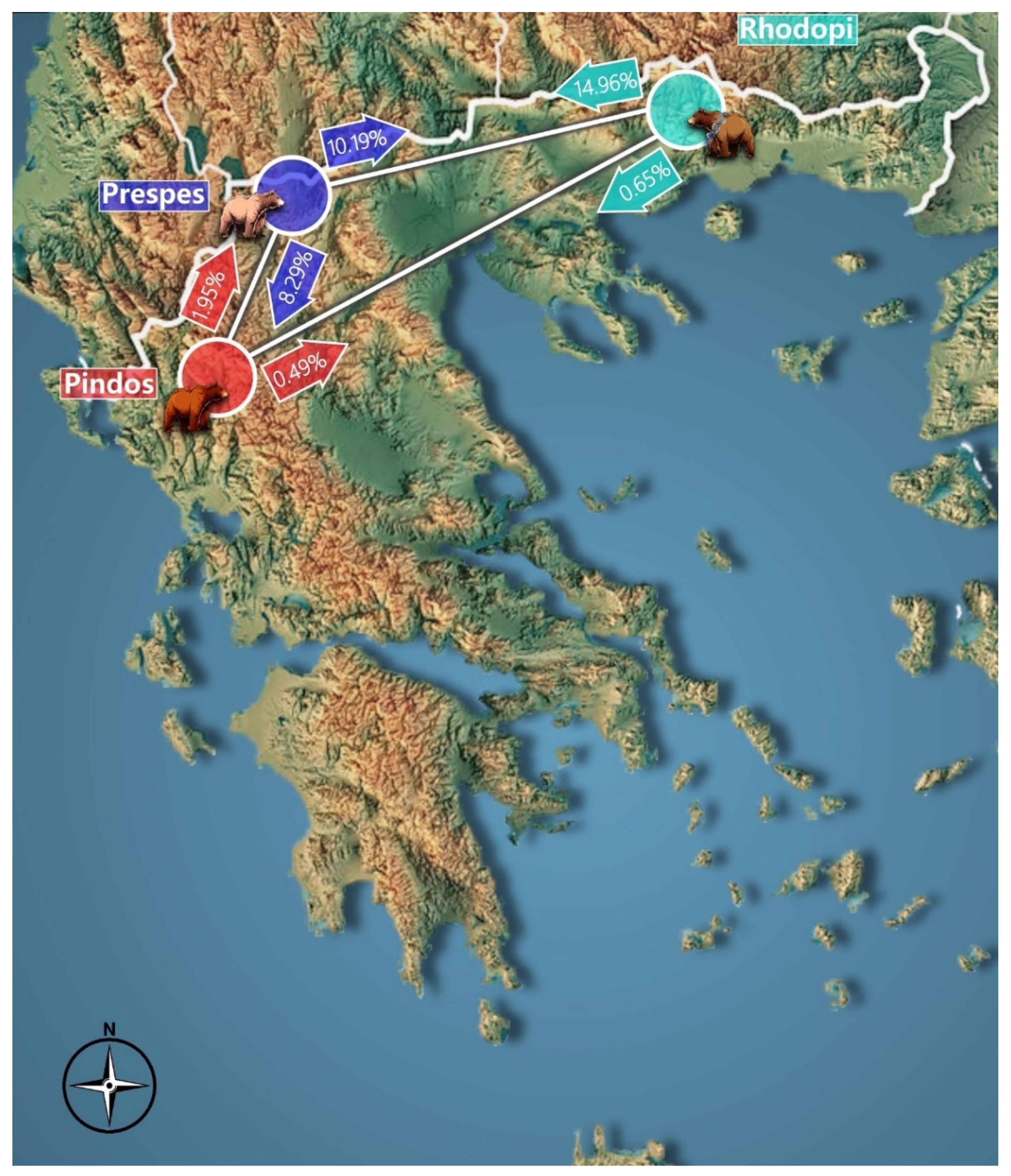
- Evidence of possible connectivity and migration of bears between the abovementioned study areas.
2. Materials and Methods
2.1. Sampling
2.2. DNA Extraction
2.3. PCR Amplification
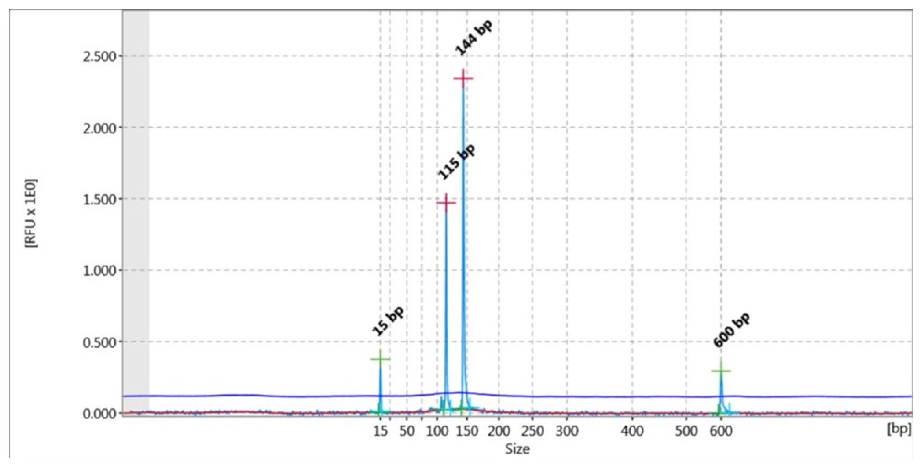
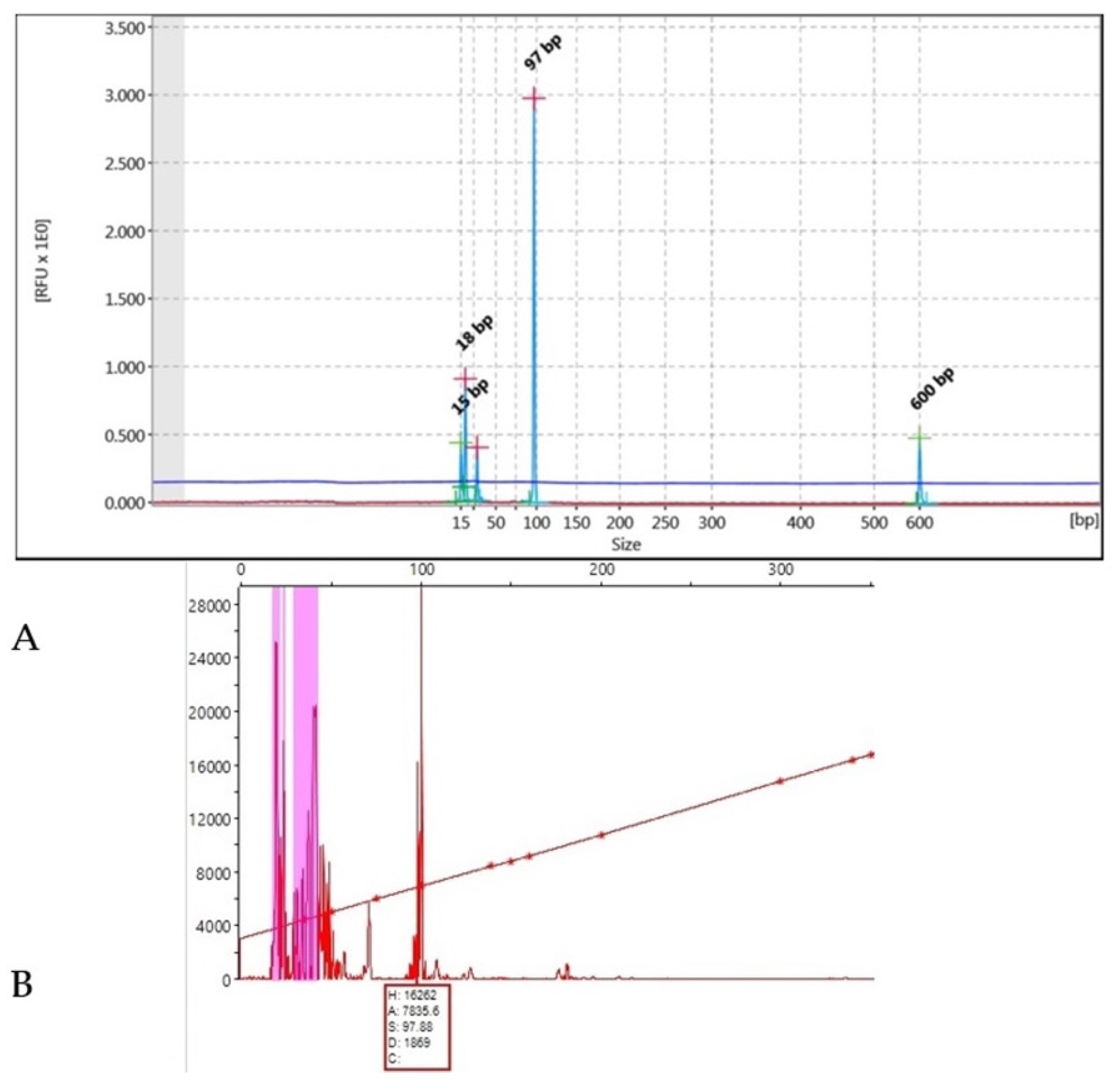
2.4. Capillary Electrophoresis
2.5. DNA Fragment Analysis
2.6. Statistical and Computational Analysis
3. Results
3.1. Samples That Were Analysed
3.2. Unique Genotypes and Sex Ratio
3.3. Genetic Diversity
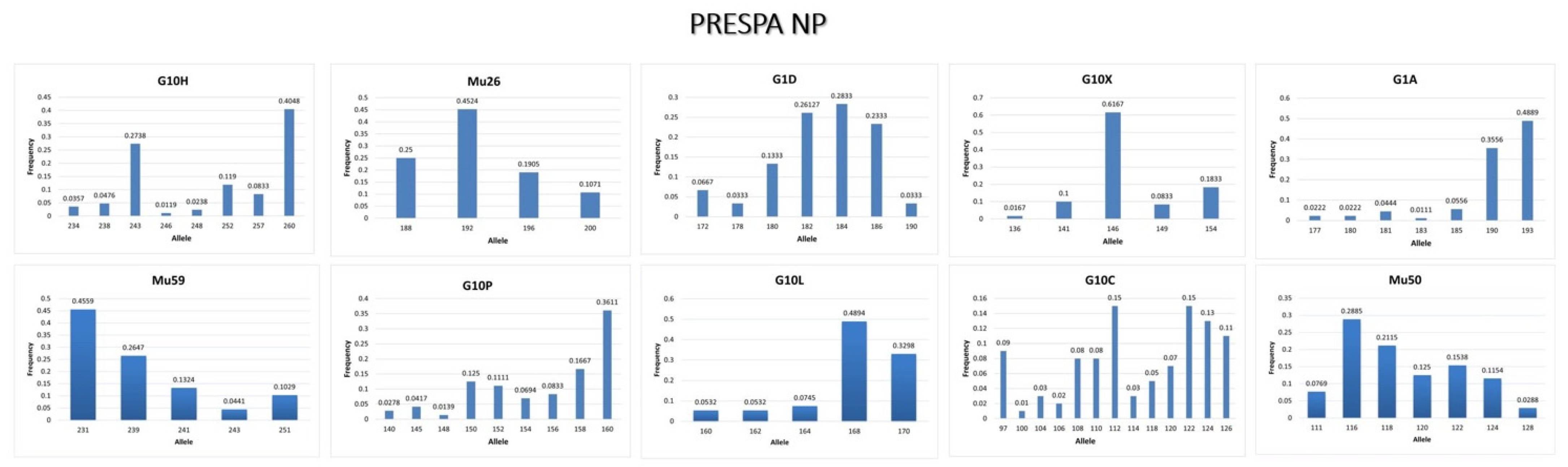
3.3.1. Prespa NP
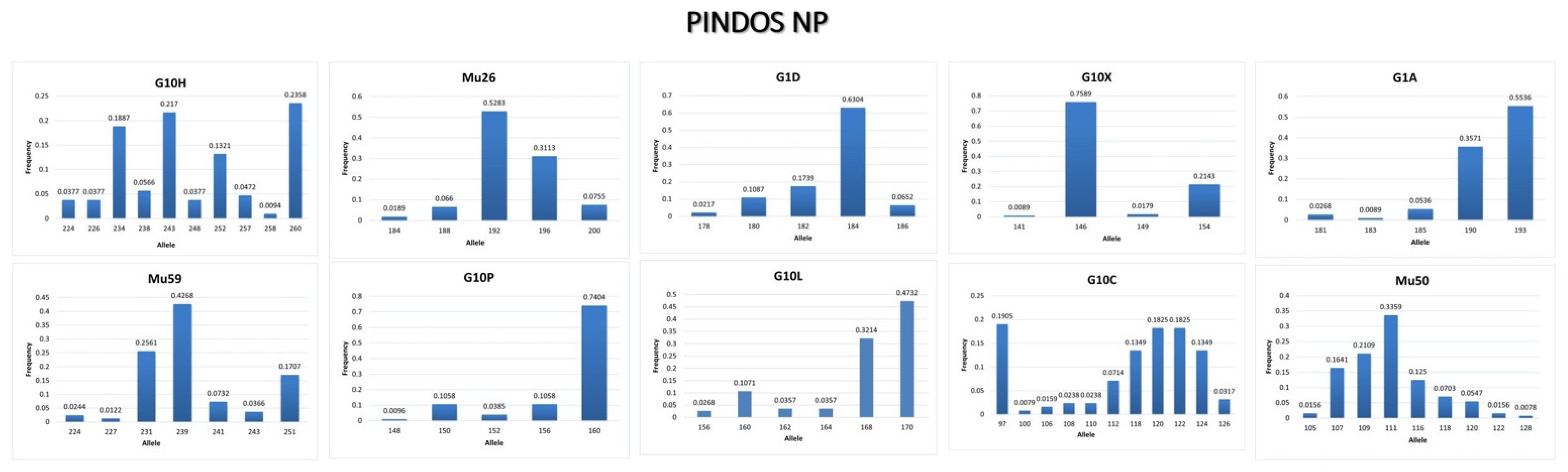
3.3.2. Pindos NP
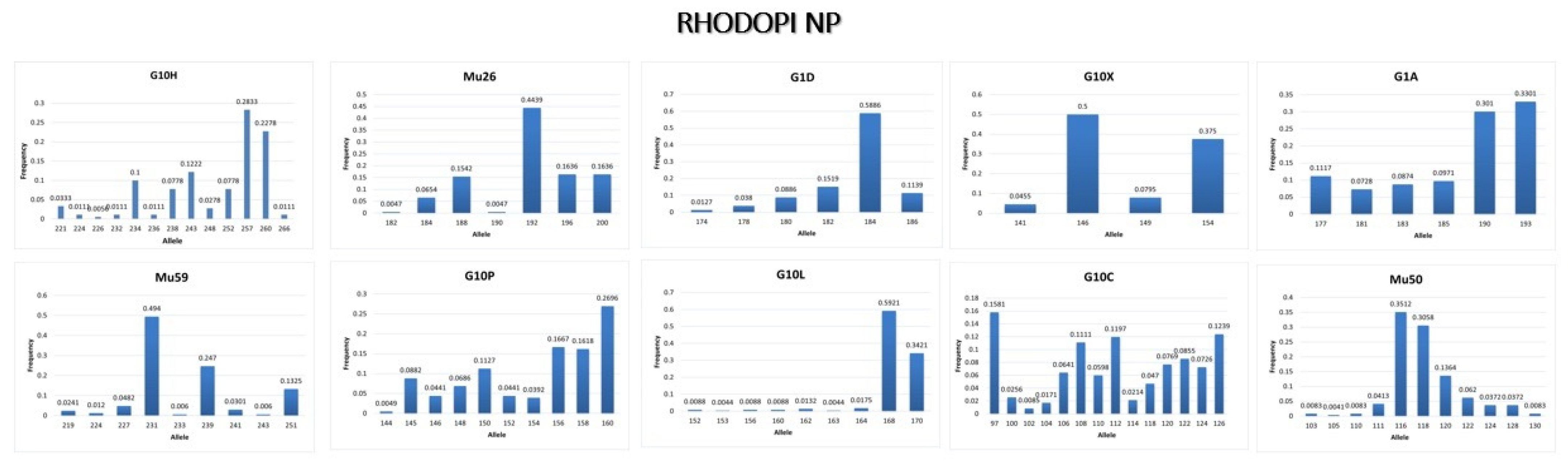
3.3.3. Rhodopi NP
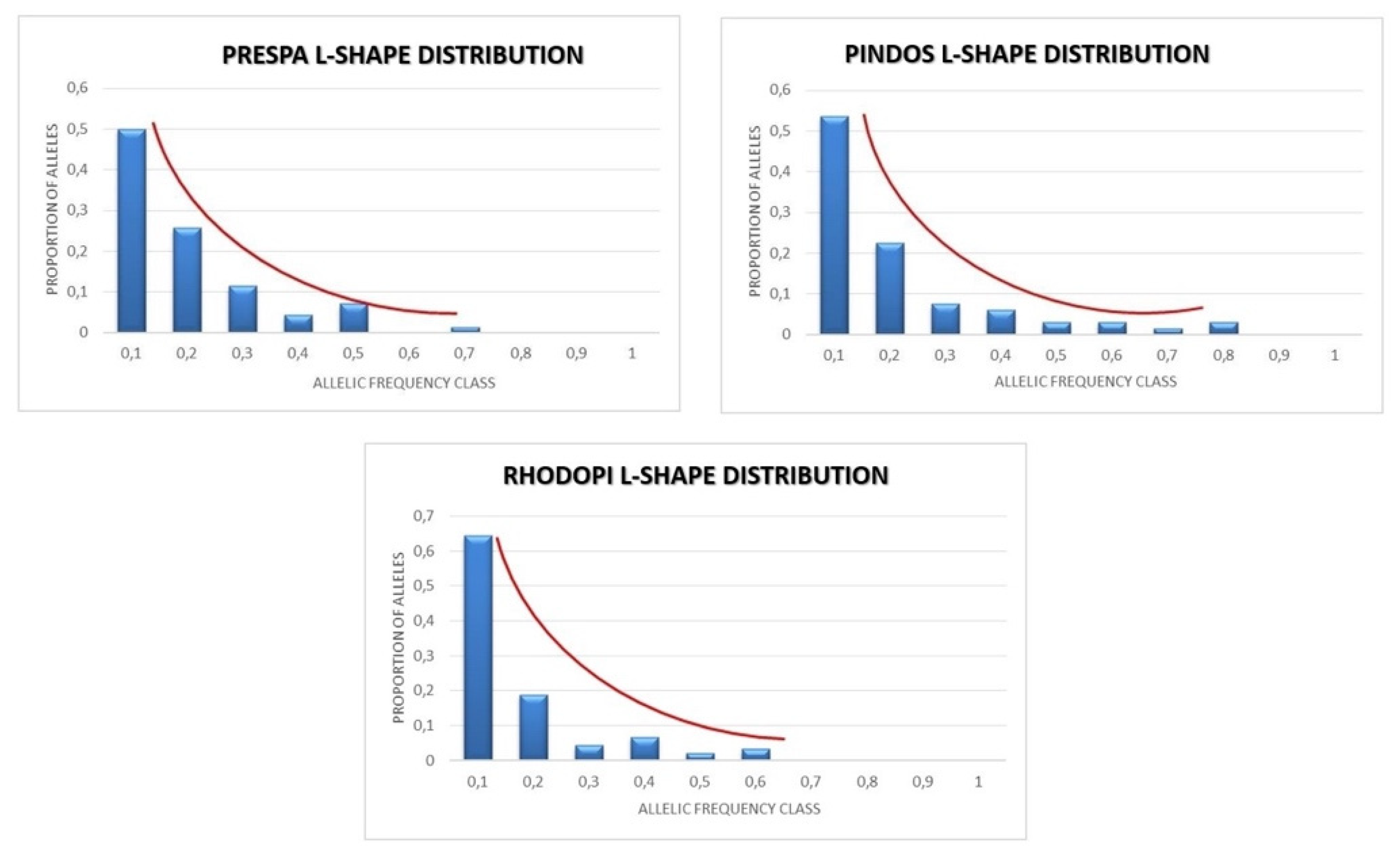
3.4. Bottleneck
3.5. Estimates of the Census Population Size (Nc) and Effective Population Size (Ne) in Prespa, Pindos, and Rhodopi NP
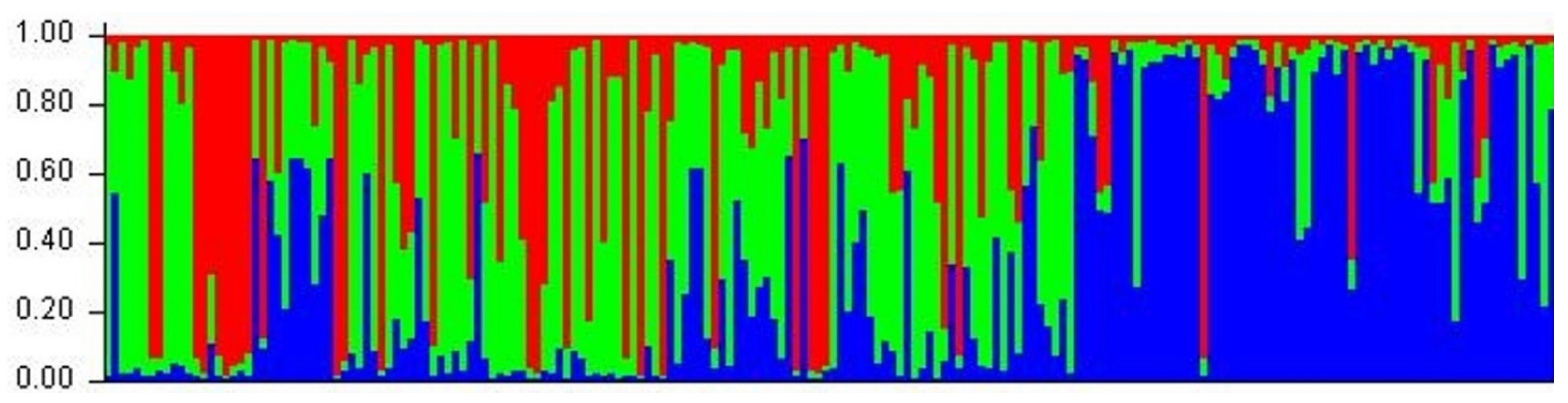
3.6. Inference of Population Genetic Structure
4. Discussion
4.1. Conclusions from the Genetic Analysis in Prespa NP
4.2. Conclusions from the Genetic Analysis in Pindos NP
4.3. Conclusions from the Genetic Analysis in Rhodopi NP
4.4. Comparison of Genetic Data from the Three Project Areas
Supplementary Materials
Author Contributions
Funding
Institutional Review Board Statement
Informed Consent Statement
Data Availability Statement
Acknowledgments
Conflicts of Interest
References
- Kaczensky, P.; Chapron, G.; von Arx, M.; Huber, D.; Andrén, H.; Linnell, J.; Adamec, M.; Álvares, F.; Anders, O.; Balciauskas, L.; et al. Status, Management and Distribution of Large Carnivores–Bear, Lynx, Wolf & Wolverine–in Europe; European Commission: Brussels, Belgium, 2013. [Google Scholar]
- Servheen, C.; Herrero, S. The Status Survey and Conservation Action Plan—Bears—Ecology of Grizzly Bears in the Greater Yellowstone Ecosystem View Project Factors Influencing Grizzly Bear Attacks on Park Visitors View Project; IUCN: Gland, Switzerland, 1999. [Google Scholar]
- Karamanlidis, A.A.; Drosopoulou, E.; de Hernando, M.G.; Georgiadis, L.; Krambokoukis, L.; Pllaha, S.; Zedrosser, A.; Scouras, Z. Noninvasive Genetic Studies of Brown Bears Using Power Poles. Eur. J. Wildl. Res. 2010, 56, 693–702. [Google Scholar] [CrossRef]
- Karamanlidis, A.A.; Skrbinšek, T.; de Gabriel Hernando, M.; Krambokoukis, L.; Munoz-Fuentes, V.; Bailey, Z.; Nowak, C.; Stronen, A.V. History-Driven Population Structure and Asymmetric Gene Flow in a Recovering Large Carnivore at the Rear-Edge of Its European Range. Heredity 2018, 120, 168–182. [Google Scholar] [CrossRef] [PubMed]
- Ashrafzadeh, M.R.; Khosravi, R.; Mohammadi, A.; Naghipour, A.A.; Khoshnamvand, H.; Haidarian, M.; Penteriani, V. Modeling Climate Change Impacts on the Distribution of an Endangered Brown Bear Population in Its Critical Habitat in Iran. Sci. Total Environ. 2022, 837, 155753. [Google Scholar] [CrossRef] [PubMed]
- Mertzanis, G. Assessment of the Distribution, Population Size and Activity of the Brown Bear (Ursus Arctos L.) Subpopulation with the Use of IR Cameras, Genetic Analyses and Biosigns in the Area of Amyndaio, & Florina—NW Greece; Technical Report A2; NGO Callisto: Thessaloniki, Greece, 2018. [Google Scholar]
- Mertzanis, G.; Giannakopoulos, A.; Pylidis, C. Status of the Brown Bear Ursus Arctos (Linnaeus, 1758) in Greece. In Red Data Book of Threatened Vertebrates of Greece; Hellenic Zoological Society: Athens, Greece, 2009. [Google Scholar]
- Karamanlidis, A.A. 1st Genetic evaluation of the brown bear (Ursus arctos) in Greece. Final report to the Hellenic Ministry of Environment, Energy and Climate Cange (In Greek). Hell. Bear Regist. 2011. [Google Scholar] [CrossRef]
- Pylidis, C.; Anijalg, P.; Saarma, U.; Dawson, D.A.; Karaiskou, N.; Butlin, R.; Mertzanis, Y.; Giannakopoulos, A.; Iliopoulos, Y.; Krupa, A.; et al. Multisource Noninvasive Genetics of Brown Bears (Ursus Arctos) in Greece Reveals a Highly Structured Population and a New Matrilineal Contact Zone in Southern Europe. Ecol. Evol. 2021, 11, 6427–6443. [Google Scholar] [CrossRef]
- Can, Ö.E.; D’Cruze, N.; Garshelis, D.L.; Beecham, J.; Macdonald, D.W. Resolving Human-Bear Conflict: A Global Survey of Countries, Experts, and Key Factors. Conserv. Lett. 2014, 7, 501–513. [Google Scholar] [CrossRef]
- Nyhus, P.J. Human–Wildlife Conflict and Coexistence. Annu. Rev. Environ. Resour. Coexistence 2016, 41, 143–171. [Google Scholar] [CrossRef]
- Long, R.A.; MacKay, P.; Ray, J.; Zielinski, W. Nonivasive Survey Methods for Carnivores; Island Press: Washington, DC, USA, 2008. [Google Scholar]
- Nichols, J.D.; Karanth, K.U. Camera Traps in Animal Ecology: Methods and Analyses; O’Connell, A.F., Ed.; Springer: New York, NY, USA, 2011. [Google Scholar]
- Kelly, M.J.; Betsch, J.; Wultsch, C.; Mesa, B.; Mills, L.S. Noninvasive Sampling for Carnivores. In Carnivore Ecology and Conservation: A Handbook of Techniques; Oxford University Press: Oxford, UK, 2012. [Google Scholar]
- Scarpulla, E.; Boattini, A.; Cozzo, M.; Giangregorio, P.; Ciucci, P.; Mucci, N.; Randi, E.; Davoli, F. First Core Microsatellite Panel Identification in Apennine Brown Bears (Ursus Arctos Marsicanus): A Collaborative Approach. BMC Genom. 2021, 22, 623. [Google Scholar] [CrossRef]
- Schwartz, M.K.; Luikart, G.; Waples, R.S. Genetic Monitoring as a Promising Tool for Conservation and Management. Trends Ecol. Evol. 2007, 22, 25–33. [Google Scholar] [CrossRef]
- Belant, J.L. A Hairsnare for Forest Carnivores. In Wildlife Society Bulletin, 31st ed.; Wiley: Hoboken, NJ, USA, 2003. [Google Scholar]
- Long, R.A.; Donovan, T.M.; Mackay, P.; Zielinski, W.J.; Buzas, J.S. Comparing Scat Detection Dogs, Cameras, and Hair Snares for Surveying Carnivores. J. Wildl. Manag. 2007, 71, 2018–2025. [Google Scholar] [CrossRef]
- Castro-Arellano, I.; Madrid-Luna, C.; Lacher, T.E.; León-Paniagua, L. Hair-Trap Efficacy for Detecting Mammalian Carnivores in the Tropics. J. Wildl. Manag. 2008, 72, 1405–1412. [Google Scholar] [CrossRef]
- Taberlet, P.; Camarra, J.-J.; Griffin, S.; Uhrès, E.; Hanotte, O.; Waits, L.P.; Dubois-Paganon, C.; Burke, T.; Bouvet, J. Noninvasive Genetic Tracking of the Endangered Pyrenean Brown Bear Population. Mol. Ecol. 1997, 6, 869–876. [Google Scholar] [CrossRef]
- Poole, K.G.; Mowat, G.; Fear, D.A. DNA-Based Population Estimate for Grizzly Bears Ursus Arctos in Northeastern British Columbia, Canada. Wildl. Biol. 2001, 7, 105–115. [Google Scholar] [CrossRef]
- Boulanger, J.; McLELLAN, B.N.; Woods, J.G.; Proctor, M.F.; Strobeck, C. Sampling Design and Bias in DNA-Based Capture-Mark-Recapture Population and Density Estimates of Grizzly Bears. J. Wildl. Manag. 2004, 68, 457–469. [Google Scholar] [CrossRef]
- Allendorf, F.W.; Christiansen, F.B.; Dobson, T.; Eanes, W.F.; Frydenberg, O. Electrophoretic Variation in Large Mammals. I. The Polar Bear, Thalarctos Maritimus. Hereditas 1979, 91, 19–22. [Google Scholar] [CrossRef]
- Guichoux, E.; Lagache, L.; Wagner, S.; Chaumeil, P.; Léger, P.; Lepais, O.; Lepoittevin, C.; Malausa, T.; Revardel, E.; Salin, F.; et al. Current Trends in Microsatellite Genotyping. Mol. Ecol. Resour. 2011, 11, 591–611. [Google Scholar] [CrossRef]
- Karamanlidis, A.A.; Youlatos, D.; Sgardelis, S.; Scouras, Z. Using Sign at Power Poles to Document Presence of Bears in Greece. Ursus 2007, 18, 54–61. [Google Scholar] [CrossRef]
- Karamanlidis, A.A.; de Gabriel Hernando, M.; Krambokoukis, L.; Gimenez, O. Evidence of a Large Carnivore Population Recovery: Counting Bears in Greece. J. Nat. Conserv. 2015, 27, 10–17. [Google Scholar] [CrossRef]
- Bellemain, E.; Taberlet, P. Improved Noninvasive Genotyping Method: Application to Brown Bear (Ursus Arctos) Faeces. Mol. Ecol. Notes 2004, 4, 519–522. [Google Scholar] [CrossRef]
- Paetkau, D.; Strobeck, C. Ecological Genetic Studies of Bears Using Microsatellite Analysis. Ursus 1998, 10, 299–306. [Google Scholar]
- Taberlet, P.; Griffin, S.; Goossens, B.; Questiau, S.; Manceau, V.; Escaravage, N.; Waits, L.P.; Bouvet, J. Reliable Genotyping of Samples with Very Low DNA Quantities Using PCR. Nucleic Acids Res. 1996, 24, 3189–3194. [Google Scholar] [CrossRef]
- Pagès, M.; Maudet, C.; Bellemain, E.; Taberlet, P.; Hughes, S.; Hänni, C. A System for Sex Determination from Degraded DNA: A Useful Tool for Palaeogenetics and Conservation Genetics of Ursids. Conserv. Genet. 2009, 10, 897–907. [Google Scholar] [CrossRef]
- Roon, D.A.; Thomas, M.E.; Kendall, K.C.; Waits, L.P. Evaluating Mixed Samples as a Source of Error in Non-Invasive Genetic Studies Using Microsatellites. Mol. Ecol. 2005, 14, 195–201. [Google Scholar] [CrossRef]
- Paetkau, D. An Empirical Exploration of Data Quality in DNA-Based Population Inventories. Mol. Ecol. 2003, 12, 1375–1387. [Google Scholar] [CrossRef]
- Miller, C.R.; Joyce, P.; Waits, L.P. Assessing Allelic Dropout and Genotype Reliability Using Maximum Likelihood. Genetics 2002, 160, 357–366. [Google Scholar] [CrossRef]
- Van Oosterhout, C.; Hutchinson, W.F.; Wills, D.P.M.; Shipley, P. MICRO-CHECKER: Software for Identifying and Correcting Genotyping Errors in Microsatellite Data. Mol. Ecol. Notes 2004, 4, 535–538. [Google Scholar] [CrossRef]
- Valière, N. Gimlet: A Computer Program for Analysing Genetic Individual Identification Data. Mol. Ecol. Notes 2002, 2, 377–379. [Google Scholar] [CrossRef]
- Tessier, C.; David, J.; This, P.; Boursiquot, J.M.; Charrier, A. Optimization of the Choice of Molecular Markers for Varietal Identification in Vitis vinifera L. Theor. Appl. Genet. 1999, 98, 171–177. [Google Scholar] [CrossRef]
- Kalinowski, S.T.; Taper, M.L.; Marshall, T.C. Revising How the Computer Program CERVUS Accommodates Genotyping Error Increases Success in Paternity Assignment. Mol. Ecol. 2007, 16, 1099–1106. [Google Scholar] [CrossRef]
- McKelvey, K.S.; Schwartz, M.K. DROPOUT: A Program to Identify Problem Loci and Samples for Noninvasive Genetic Samples in a Capture-Mark-Recapture Framework. Mol. Ecol. Notes 2005, 5, 716–718. [Google Scholar] [CrossRef]
- Rousset, F. GENEPOP’007: A Complete Re-Implementation of the GENEPOP Software for Windows and Linux. Mol. Ecol. Resour. 2008, 8, 103–106. [Google Scholar] [CrossRef] [PubMed]
- Piry, S.; Luikart, G.; Cornuet, J.M. BOTTLENECK: A Computer Program for Detecting Recent Reductions in the Effective Population Size Using Allele Frequency Data. J. Hered. 1999, 90, 502–503. [Google Scholar] [CrossRef]
- Tóth, B.; Khosravi, R.; Ashrafzadeh, M.R.; Bagi, Z.; Fehér, M.; Bársony, P.; Kovács, G.; Kusza, S. Genetic Diversity and Structure of Common Carp (Cyprinus Carpio L.) in the Centre of Carpathian Basin: Implications for Conservation. Genes 2020, 11, 1268. [Google Scholar] [CrossRef] [PubMed]
- Peel, D.; Peel, S.L.; Ovenden, J.R. NeEstimator: Software for Estimating Effective Population Size; NeEstimator software | Molecular Fisheries Laboratory; Department of Primary Industries and Fisheries, University of QueensLand: Brisbane, Australia, 2003. [Google Scholar]
- Pennell, M.W.; Stansbury, C.R.; Waits, L.P.; Miller, C.R. Capwire: A R Package for Estimating Population Census Size from Non-Invasive Genetic Sampling. Mol. Ecol. Resour. 2013, 13, 154–157. [Google Scholar] [CrossRef]
- Puechmaille, S.J.; Petit, E.J. Empirical Evaluation of Non-Invasive Capture–Mark–Recapture Estimation of Population Size Based on a Single Sampling Session. J. Appl. Ecol. 2007, 44, 843–852. [Google Scholar] [CrossRef]
- Arrendal, J.; Vilà, C.; Björklund, M. Reliability of Noninvasive Genetic Census of Otters Compared to Field Censuses. Conserv. Genet. 2007, 8, 1097–1107. [Google Scholar] [CrossRef]
- Piggott, M.P.; Taylor, A.C. Remote Collection of Animal DNA and Its Applications in Conservation Management and Understanding the Population Biology of Rare and Cryptic Species. Wildl. Res. 2003, 30, 1–13. [Google Scholar] [CrossRef]
- Miller, C.R.; Joyce, P.; Waits, L.P. A New Method for Estimating the Size of Small Populations from Genetic Mark-Recapture Data. Mol. Ecol. 2005, 14, 1991–2005. [Google Scholar] [CrossRef]
- Boulanger, J.; McLellan, B. Closure Violation in DNA-Based Mark-Recapture Estimation of Grizzly Bear Populations. Can. J. Zool. 2001, 79, 642–651. [Google Scholar] [CrossRef]
- Botstein, D.; White, R.L.; Skolnick, M.; Davis, R.W. Construction of a Genetic Linkage Map in Man Using Restriction Fragment Length Polymorphisms. Am. J. Hum. Genet. 1980, 32, 314. [Google Scholar]
- Weir, B.S.; Cockerham, C.C. Estimating F-Statistics for the Analysis of Population Structure. Evolution 1984, 38, 1358–1370. [Google Scholar] [CrossRef]
- Evanno, G.; Regnaut, S.; Goudet, J. Detecting the Number of Clusters of Individuals Using the Software Structure: A Simulation Study. Mol. Ecol. 2005, 14, 2611–2620. [Google Scholar] [CrossRef]
- Wilson, G.A.; Rannala, B. Bayesian Inference of Recent Migration Rates Using Multilocus Genotypes. Genetics 2003, 163, 1177–1191. [Google Scholar] [CrossRef]
- Ellengren, H.; Johansson, M.; Sandberg, K.; Andersson, L. Cloning of Highly Polymorphic Microsatellites in the Horse. Anim. Genet. 1992, 23, 133–142. [Google Scholar] [CrossRef]
- Lander, E.S.; Botstein, S. Mapping Mendelian Factors Underlying Quantitative Traits Using RFLP Linkage Maps. Genetics 1989, 121, 185. [Google Scholar] [CrossRef]
- Hildebrand, C.E.; Torney, D.C.; Wagner, R.P. Informativeness of Polymorphic DNA Markers. Los Alamos Sci. 1992, 20, 100–102. [Google Scholar]
- Wright, S. The Interpretation of Population Structure by F-Statistics with Special Regard to Systems of Mating. Evolution 1965, 19, 395. [Google Scholar] [CrossRef]
- Hartl, D.L. A Primer of Population Genetics, 3rd ed.; Sinauer Associates Incorporated: Sunderland, MA, USA, 2000. [Google Scholar]
- Kimura, M.; Ohta, T. Stepwise Mutation Model and Distribution of Allelic Frequencies in a Finite Population. Proc. Natl. Acad. Sci USA 1978, 75, 2868. [Google Scholar] [CrossRef]
- Tsaparis, D.; Karaiskou, N.; Mertzanis, Y.; Triantafyllidis, A. Non-Invasive Genetic Study and Population Monitoring of the Brown Bear (Ursus Arctos) (Mammalia: Ursidae) in Kastoria Region—Greece. J. Nat. Hist. 2015, 49, 393–410. [Google Scholar] [CrossRef]
- Kasarda, R.; Vostrý, L.; Vostrá-Vydrová, H.; Candráková, K.; Moravčíková, N. Food Resources Biodiversity: The Case of Local Cattle in Slovakia. Sustainability 2021, 13, 1296. [Google Scholar] [CrossRef]
- Kendall, W.L. Robustness of Closed Capture-Recapture Methods to Violations of the Closure Assumption. Ecology 1999, 80, 2517. [Google Scholar] [CrossRef]
- Green, G.I.; Mattson, D.J. Tree Rubbing by Yellowstone Grizzly Bears Ursus Arctos. Wildl. Biol. 2003, 9, 1–9. [Google Scholar] [CrossRef]
- Palstra, F.P.; Ruzzante, D.E. Genetic Estimates of Contemporary Effective Population Size: What Can They Tell Us about the Importance of Genetic Stochasticity for Wild Population Persistence? Mol. Ecol. 2008, 17, 3428–3447. [Google Scholar] [CrossRef]
- Ferchaud, A.L.; Perrier, C.; April, J.; Hernandez, C.; Dionne, M.; Bernatchez, L. Making Sense of the Relationships between Ne, Nb and Nc towards Defining Conservation Thresholds in Atlantic Salmon (Salmo Salar). Heredity 2016, 117, 268–278. [Google Scholar] [CrossRef]
- Boitani, L.; Powell, R.A. Carnivore Ecology and Conservation: A Handbook of Techniques Book Review. J. Mammal. 2013, 94, 1471–1472. [Google Scholar]
- Waits, L.P.; Paetkau, D. Allen Press Noninvasive Genetic Sampling Tools for Wildlife Biologists: A Review of Applications and Recommendations for Accurate Data Collection. Source: J. Wildl. Manag. 2005, 69, 1419–1433. [Google Scholar]
- Pérez, T.; Naves, J.; Vázquez, J.F.; Seijas, J.; Corao, A.; Albornoz, J.; Domínguez, A. Evidence for Improved Connectivity between Cantabrian Brown Bear Subpopulations. Ursus 2010, 21, 104–108. [Google Scholar] [CrossRef]
- Sawaya, M.A.; Stetz, J.B.; Clevenger, A.P.; Gibeau, M.L.; Kalinowski, S.T. Estimating Grizzly and Black Bear Population Abundance and Trend in Banff National Park Using Noninvasive Genetic Sampling. PLoS ONE 2012, 7, e34777. [Google Scholar] [CrossRef]
- Kronforst, M.R.; Fleming, T.H. Lack of Genetic Differentiation among Widely Spaced Subpopulations of a Butterfly with Home Range Behaviour. Heredity 2001, 86, 243–250. [Google Scholar] [CrossRef]
- Woods, J.G.; Paetkau, D.; Lewis, D.; McLellan, B.N.; Proctor, M.; Strobeck, C. Genetic Tagging Free-Ranging Black and Brown Bears. Wildl. Soc. Bull. 1999, 27, 616–627. [Google Scholar]
- Waits, L.P.; Luikart, G.; Taberlet, P. Estimating the Probability of Identity among Genotypes in Natural Populations: Cautions and Guidelines. Mol. Ecol. 2001, 10, 249–256. [Google Scholar] [CrossRef] [PubMed]
- Bartoń, K.A.; Zwijacz-Kozica, T.; Zięba, F.; Sergiel, A.; Selva, N. Bears without Borders: Long-Distance Movement in Human-Dominated Landscapes. Glob. Ecol. Conserv. 2019, 17, e00541. [Google Scholar] [CrossRef]


| Primer Sequence | Length (bp) | References | |
|---|---|---|---|
| G10H F | 5′-CCCAACAAGAAGACCACTGTAA-3′ | 221–257 | [28] |
| G10H R | 5′-CCAGAGACCACCAAGTAGGATA-3′ | ||
| G10L F | 5′-TGTACTGATTTAATTCACATTTCCC-3′ | 153–163 | [28] |
| G10L R | 5′-GAAGATACAGAAACCTACCCATGC-3′ | ||
| Mu50 F | 5′-GTCTCTGTCATTTCCCCATC-3′ | 110–130 | [27] |
| Mu50 R | 5′-AACCTGGAACAAAAATTAACAC-3′ | ||
| Mu26 F | 5′-GCCTCAAATGACAAGATTTC-3′ | 182–200 | [20] |
| Mu26 R | 5′-TCAATTAAAATAGGAAGCAGC-3′ | ||
| G10P F | 5′-TACATAGGAGGAAGAAAGATGG-3′ | 145–159 | [28] |
| G10P R | 5′-AAAAGGCCTAAGCTACATCG-3′ | ||
| Mu59 F | 5′-TGCTGCTTTGGGACATTGTAA-3′ | 219–251 | [20] |
| Mu59 R | 5′-CAATCAGGCATGGGGAAGAA-3′ | ||
| G10C F | 5′-AAAGCAGAAGGCCTTGATTTCCTG-3′ | 97–116 | [28] |
| G10C R | 5′-GGGACATAAACACCGAGACAGC-3′ | ||
| G1D F | 5′-ATCTGTGGGTTTATAGGTTACA-3′ | 172–184 | [28] |
| G1D R | 5′-CTACTCTTCCTACTCTTTAAGAG-3′ | ||
| G10X F | 5′-CCCTGGTAACCACAAATCTCT-3′ | 132–154 | [20,28] |
| G10X R | 5′-TCAGTTATCTGTGAAATCAAAA-3′ | ||
| G1A F | 5′-GACCCTGCATACTCTCCTCTGATG-3′ | 180–190 | [28] |
| G1A R | 5′-GCACTGTCCTGCGTAGAAGTGAC-3′ | ||
| SRY-F | 5′ -TGGTCTCGTGATCAAAGGCGC-3′ | 115 | [30] |
| SRY-R | 5′-GCCATTTTTCGGCTTCCGTAAG-3′ | ||
| ZF-F | 5′-GACAGCTGAACAAGGGTTG-3′ | 144 | [30] |
| ZF-R | 5′-GCTTCTCGCCGGTATGGATG-3′ | ||
| Locus | Individuals | Heterozygotes | Homozygotes | Number of Alleles |
|---|---|---|---|---|
| G10H | 42 | 13 | 29 | 8 |
| Mu26 | 39 | 25 | 14 | 4 |
| G1D | 30 | 11 | 19 | 7 |
| G10X | 30 | 17 | 13 | 5 |
| G1A | 45 | 23 | 22 | 7 |
| G10P | 36 | 21 | 15 | 9 |
| G10C | 50 | 34 | 16 | 13 |
| Mu59 | 34 | 5 | 29 | 5 |
| G10L | 47 | 32 | 15 | 5 |
| Mu50 | 52 | 44 | 8 | 7 |
| Locus | A | R (bp) | He | Ho | pHW | Fis | PID-sib | Fnull | PIC |
|---|---|---|---|---|---|---|---|---|---|
| G10H | 8 | 234–260 | 0.74 | 0.25 | 0.0000 | 0.5873 | 4.088 × 10⁻¹ | 0.4320 | 0.699 |
| MU26 | 4 | 188–200 | 0.69 | 0.47 | 0.0550 | 0.1430 | 1.820 × 10⁻¹ | 0.0788 | 0.633 |
| G1D | 7 | 172–190 | 0.79 | 0.21 | 0.0000 | 0.5501 | 6.758 × 10⁻² | 0.3696 | 0.763 |
| G10X | 5 | 136–154 | 0.57 | 0.32 | 0.0180 | 0.0209 | 3.528 × 10⁻² | −0.0118 | 0.529 |
| G1A | 7 | 177–193 | 0.63 | 0.43 | 0.0020 | 0.1975 | 1.717 × 10⁻² | 0.1130 | 0.563 |
| G10P | 9 | 140–160 | 0.80 | 0.40 | 0.0038 | 0.2833 | 6.280 × 10⁻³ | 0.1559 | 0.777 |
| G10C | 13 | 97–126 | 0.90 | 0.64 | 0.0000 | 0.2501 | 1.930 × 10⁻³ | 0.1381 | 0.886 |
| MU59 | 5 | 231–251 | 0.69 | 0.09 | 0.0000 | 0.7931 | 8.479 × 10⁻⁴ | 0.6598 | 0.646 |
| G10L | 5 | 160–170 | 0.64 | 0.60 | 0.0000 | −0.0522 | 4.045 × 10⁻⁴ | −0.0281 | 0.581 |
| MU50 | 7 | 111–128 | 0.81 | 0.83 | 0.6495 | −0.0315 | 1.451 × 10⁻⁴ | −0.0210 | 0.788 |
| Mean | 7 | 0.73 | 0.42 | 0.28 | 0.69 |
| Locus | Individuals | Heterozygotes | Homozygotes | Number of Alleles |
|---|---|---|---|---|
| G10H | 53 | 34 | 19 | 10 |
| Mu26 | 53 | 40 | 13 | 5 |
| G1D | 23 | 9 | 14 | 5 |
| G10X | 56 | 25 | 31 | 4 |
| G1A | 56 | 34 | 22 | 5 |
| G10P | 52 | 16 | 36 | 5 |
| G10C | 63 | 57 | 6 | 11 |
| Mu59 | 41 | 19 | 22 | 7 |
| G10L | 56 | 32 | 24 | 6 |
| Mu50 | 64 | 58 | 6 | 9 |
| locus | A | R (bp) | He | Ho | pHW | Fis | PID-sib | Fnull | PIC |
|---|---|---|---|---|---|---|---|---|---|
| G10H | 10 | 234–260 | 0.84 | 0.64 | 0.0000 | 0.2402 | 3.447 × 10⁻¹ | 0.1280 | 0.814 |
| MU26 | 5 | 188–200 | 0.62 | 0.76 | 0.0000 | −0.2210 | 1.710 × 10⁻¹ | −0.1286 | 0.552 |
| G1D | 5 | 172–190 | 0.57 | 0.39 | 0.0040 | 0.3161 | 9.081 × 10⁻² | 0.2107 | 0.517 |
| G10X | 4 | 136–154 | 0.38 | 0.45 | 0.5072 | −0.1732 | 6.096 × 10⁻² | −0.0939 | 0.324 |
| G1A | 5 | 177–193 | 0.57 | 0.61 | 0.0000 | −0.0707 | 3.274 × 10⁻² | −0.0349 | 0.481 |
| G10P | 5 | 140–160 | 0.43 | 0.31 | 0.0000 | 0.2898 | 2.045 × 10⁻² | 0.2260 | 0.401 |
| G10C | 11 | 97–126 | 0.86 | 0.91 | 0.0000 | −0.0526 | 6.813 × 10⁻³ | −0.0337 | 0.836 |
| MU59 | 7 | 231–251 | 0.72 | 0.46 | 0.0001 | 0.3632 | 2.882 × 10⁻³ | 0.2086 | 0.673 |
| G10L | 6 | 160–170 | 0.66 | 0.57 | 0.0000 | 0.1404 | 1.338 × 10⁻³ | 0.0657 | 0.602 |
| MU50 | 9 | 111–128 | 0.80 | 0.91 | 0.0439 | −0.1371 | 4.976 × 10⁻⁴ | −0.0758 | 0.764 |
| Mean | 6.7 | 0.65 | 0.6 | 0.13 | 0.6 |
| Locus | Individuals | Heterozygotes | Homozygotes | Number of Alleles |
|---|---|---|---|---|
| G10H | 64 | 17 | 47 | 12 |
| Mu26 | 72 | 45 | 27 | 7 |
| G1D | 61 | 8 | 53 | 7 |
| G10X | 33 | 16 | 17 | 4 |
| G1A | 64 | 39 | 25 | 6 |
| G10P | 63 | 40 | 23 | 10 |
| G10C | 74 | 51 | 23 | 13 |
| Mu59 | 61 | 20 | 41 | 9 |
| G10L | 76 | 54 | 22 | 7 |
| Mu50 | 78 | 67 | 11 | 9 |
| Locus | A | R (bp) | He | Ho | pHW | Fis | PID-sib | Fnull | PIC |
|---|---|---|---|---|---|---|---|---|---|
| G10H | 12 | 221–266 | 0.82 | 0.27 | 0.0000 | 0.6791 | 3.554 × 10⁻¹ | 0.5208 | 0.795 |
| MU26 | 7 | 182–200 | 0.75 | 0.63 | 0.0505 | 0.1617 | 1.447 × 10⁻¹ | 0.0845 | 0.700 |
| G1D | 7 | 172–186 | 0.63 | 0.13 | 0.0000 | 0.7917 | 7.010 × 10⁻² | 0.6607 | 0.586 |
| G10X | 4 | 141–154 | 0.61 | 0.49 | 0.2855 | 0.2044 | 3.587 × 10⁻² | 0.1079 | 0.516 |
| G1A | 6 | 177–193 | 0.77 | 0.61 | 0.0000 | 0.2112 | 1.399 × 10⁻² | 0.1213 | 0.730 |
| G10P | 10 | 144–160 | 0.83 | 0.64 | 0.0000 | 0.2329 | 4.948 × 10⁻³ | 0.1286 | 0.798 |
| G10C | 13 | 97–126 | 0.90 | 0.69 | 0.0000 | 0.2339 | 1.531 × 10⁻³ | 0.1322 | 0.882 |
| MU59 | 9 | 219–251 | 0.64 | 0.33 | 0.0000 | 0.4924 | 7.273 × 10⁻⁴ | 0.3375 | 0.592 |
| G10L | 7 | 152–170 | 0.52 | 0.71 | 0.0000 | −0.3659 | 4.161 × 10⁻⁴ | −0.1676 | 0.426 |
| MU50 | 9 | 103–128 | 0.77 | 0.86 | 0.0439 | −0.1205 | 1.629 × 10⁻⁴ | −0.0691 | 0.728 |
| Mean | 8.4 | 0.72 | 0.54 | 0.3 | 0.68 |
| Population | Number of Samples with >6 loci | Different Individuals | A | He | Ho | Nc | Ne | PIC | Fis |
|---|---|---|---|---|---|---|---|---|---|
| Prespa | 59 | 53 | 7 | 0.73 | 0.42 | 191 | 35 (25–52) | 0.69 | 0.28 |
| Pindos | 77 | 65 | 6.7 | 0.65 | 0.6 | 202 | 118 (66–271) | 0.6 | 0.13 |
| Rhodopi | 121 | 77 | 8.4 | 0.72 | 0.54 | 92 | 61(47–84) | 0.68 | 0.3 |
| Area of Population | Samples | A | He | Ho | Nc | Ne | Fis | Reference |
|---|---|---|---|---|---|---|---|---|
| Prespa | 53 | 7 | 0.73 | 0.42 | 191 | 35 | 0.28 | This study |
| Kastoria | 82 | 5.8 | 0.548 | 0.584 | 219 | 39.5–49 | 0.07 | Tsaparis et al., 2015 [59] |
| Peristeri | 30 | 5.64 | 0.69 | 0.65 | 109 | 59.1 | 0.047 | Pylidis, 2021 [9] |
| Amyntaio | 56 | 6.8 | 0.582 | 0.412 | 154 | 44 | 0.25 | Mertzanis et al., 2018 [6] LIFE15NAT/GR/001108 |
| Area of Population | Samples | A | He | Ho | Nc | Ne | Fis | Reference |
|---|---|---|---|---|---|---|---|---|
| Pindos | 65 | 6.7 | 0.65 | 0.6 | 202 | 118 | 0.13 | This study |
| Pindos | 159 | 6.42 | - | 0.70 | - | 182.3 | - | Karamanlidis, 2015 [26] |
| Pindos | 47 | 5–8 | 0.76 | 0.77 | 76 | - | Karamanlidis, 2010 [2] | |
| North Pindos | 65 | 5.47 | 0.658 | 0.67 | - | 65–149.8 | - | Karamanlidis, 2018 [4] |
| South-Central Pindos | 99 | 5.76 | 0.680 | 0.68 | - | 80.5–148.7 | - | Karamanlidis, 2018 [4] |
| Pindos | 97 | 5.27 | 0.64 | 0.61 | 299 | 97.4 | 0.042 | Pylidis, 2021 [9] |
| Area of Population | Samples | A | He | Ho | Nc | Ne | Fis | Reference |
|---|---|---|---|---|---|---|---|---|
| Rhodopi | 77 | 8.4 | 0.72 | 0.54 | 92 | 61 | 0.3 | This study |
| Rhodopi | 22 | 6.09 | 0.73 | 0.71 | 91 | 42.2 | 0.021 | Pylidis, 2021 [9] |
| Rhodopi | 15 | 6.529 | 0.745 | 0.808 | - | - | - | Karamanlidis, 2018 [4] |
Publisher’s Note: MDPI stays neutral with regard to jurisdictional claims in published maps and institutional affiliations. |
© 2022 by the authors. Licensee MDPI, Basel, Switzerland. This article is an open access article distributed under the terms and conditions of the Creative Commons Attribution (CC BY) license (https://creativecommons.org/licenses/by/4.0/).
Share and Cite
Tsalazidou-Founta, T.-M.; Stasi, E.A.; Samara, M.; Mertzanis, Y.; Papathanassiou, M.; Bagos, P.G.; Psaroudas, S.; Spyrou, V.; Lazarou, Y.; Tragos, A.; et al. Genetic Analysis and Status of Brown Bear Sub-Populations in Three National Parks of Greece Functioning as Strongholds for the Species’ Conservation. Genes 2022, 13, 1388. https://doi.org/10.3390/genes13081388
Tsalazidou-Founta T-M, Stasi EA, Samara M, Mertzanis Y, Papathanassiou M, Bagos PG, Psaroudas S, Spyrou V, Lazarou Y, Tragos A, et al. Genetic Analysis and Status of Brown Bear Sub-Populations in Three National Parks of Greece Functioning as Strongholds for the Species’ Conservation. Genes. 2022; 13(8):1388. https://doi.org/10.3390/genes13081388
Chicago/Turabian StyleTsalazidou-Founta, Tzoulia-Maria, Evangelia A. Stasi, Maria Samara, Yorgos Mertzanis, Maria Papathanassiou, Pantelis G. Bagos, Spyros Psaroudas, Vasiliki Spyrou, Yorgos Lazarou, Athanasios Tragos, and et al. 2022. "Genetic Analysis and Status of Brown Bear Sub-Populations in Three National Parks of Greece Functioning as Strongholds for the Species’ Conservation" Genes 13, no. 8: 1388. https://doi.org/10.3390/genes13081388
APA StyleTsalazidou-Founta, T.-M., Stasi, E. A., Samara, M., Mertzanis, Y., Papathanassiou, M., Bagos, P. G., Psaroudas, S., Spyrou, V., Lazarou, Y., Tragos, A., Tsaknakis, Y., Grigoriadou, E., Korakis, A., Satra, M., Billinis, C., & ARCPROM project. (2022). Genetic Analysis and Status of Brown Bear Sub-Populations in Three National Parks of Greece Functioning as Strongholds for the Species’ Conservation. Genes, 13(8), 1388. https://doi.org/10.3390/genes13081388