
Precision DNA Mixture Interpretation with Single-Cell Profiling


Abstract
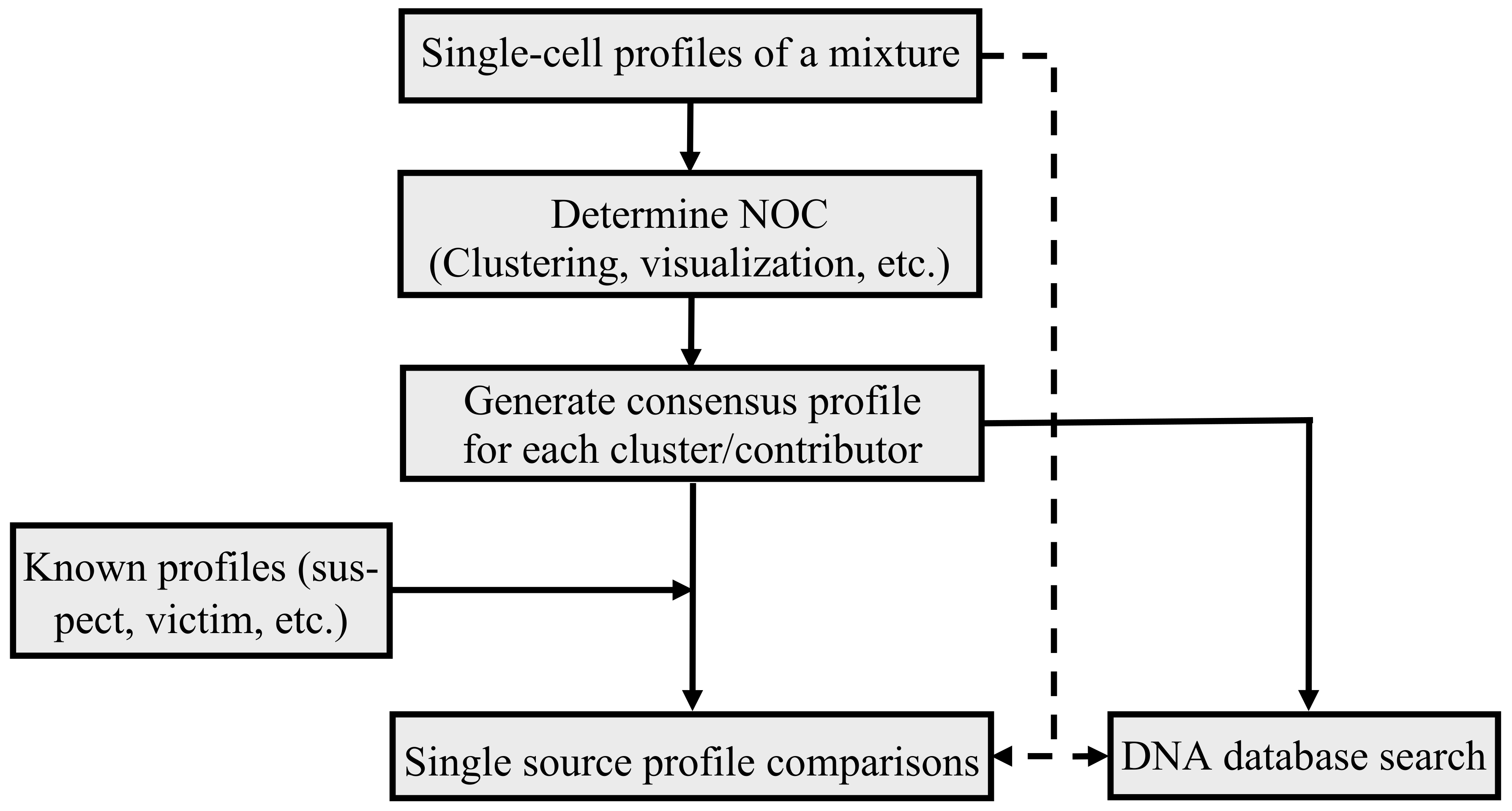
:1. Introduction
2. Methods
2.1. Simulation Methods
2.2. Clustering Single Cells
2.3. Single-Cell Profile Visualization
2.4. Consensus Method
3. Results
3.1. The Probability of Not Detecting a Contributor during Sampling
3.2. The Accuracies of NOC Estimation
3.2.1. NOC Estimation by Clustering
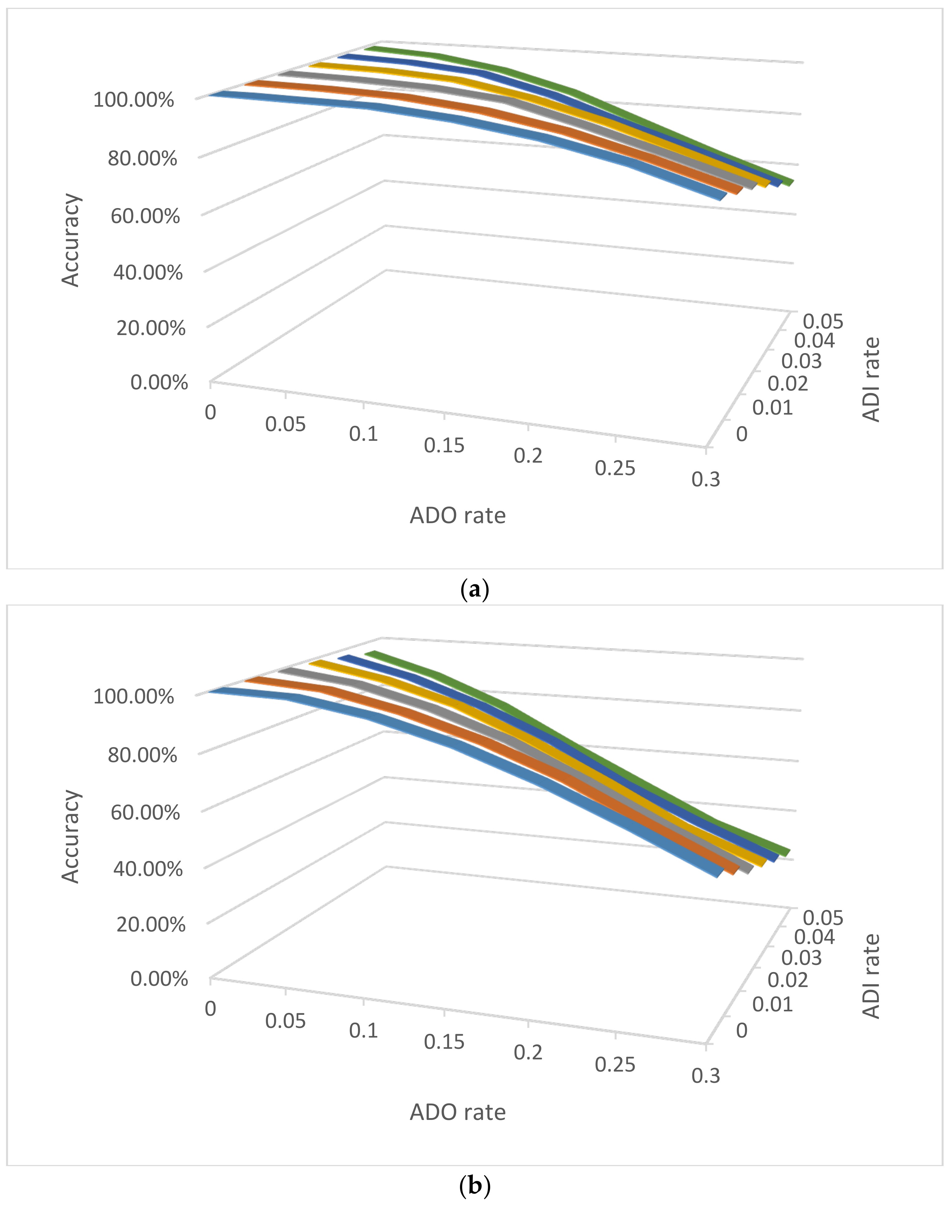
3.2.2. Impact of ADO and ADI on NOC Estimation by Clustering
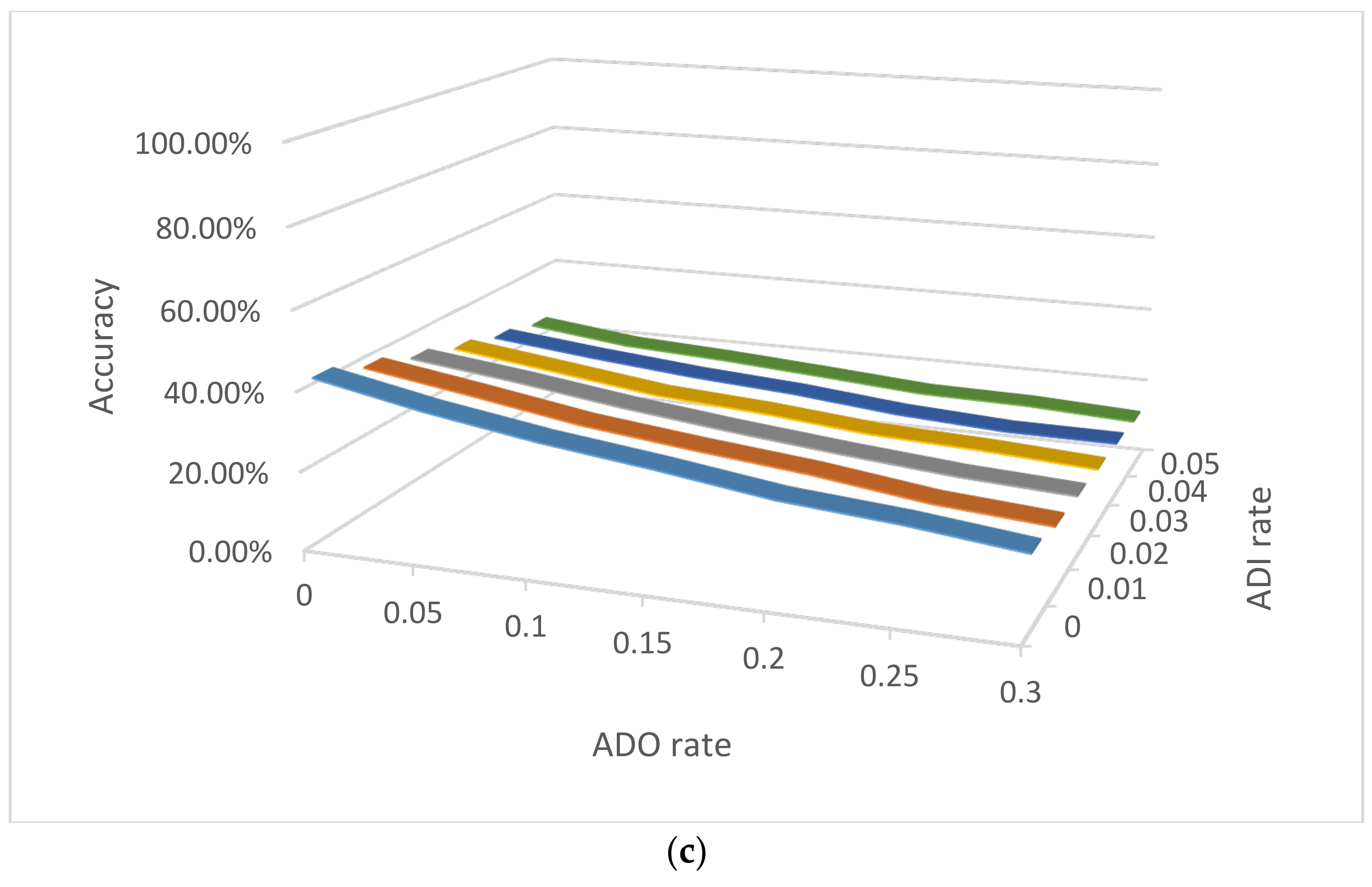
3.2.3. NOC Estimation by Visualization
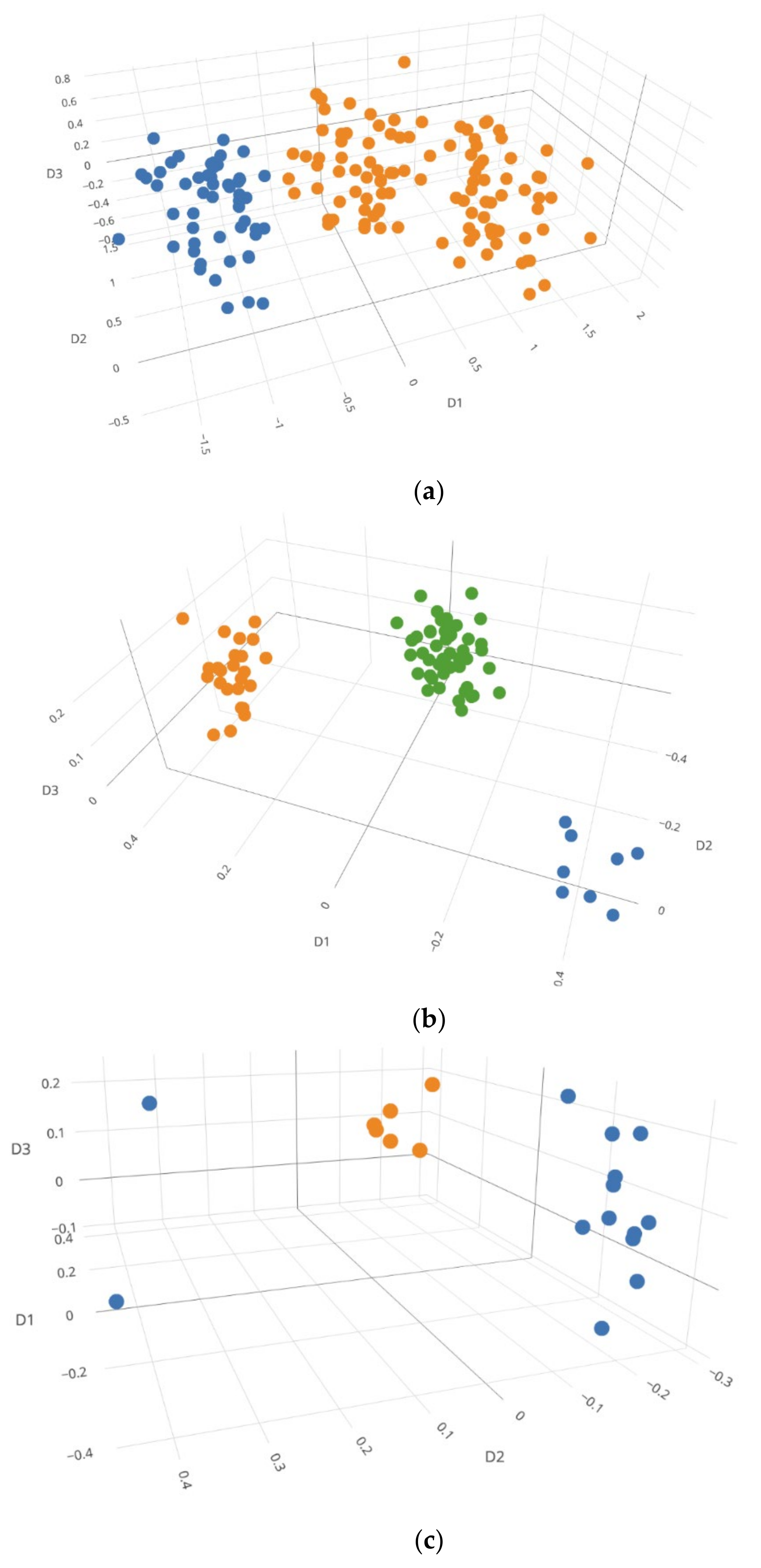
3.2.4. NOC Estimation by Identity-by-State (IBS) Distance Measure
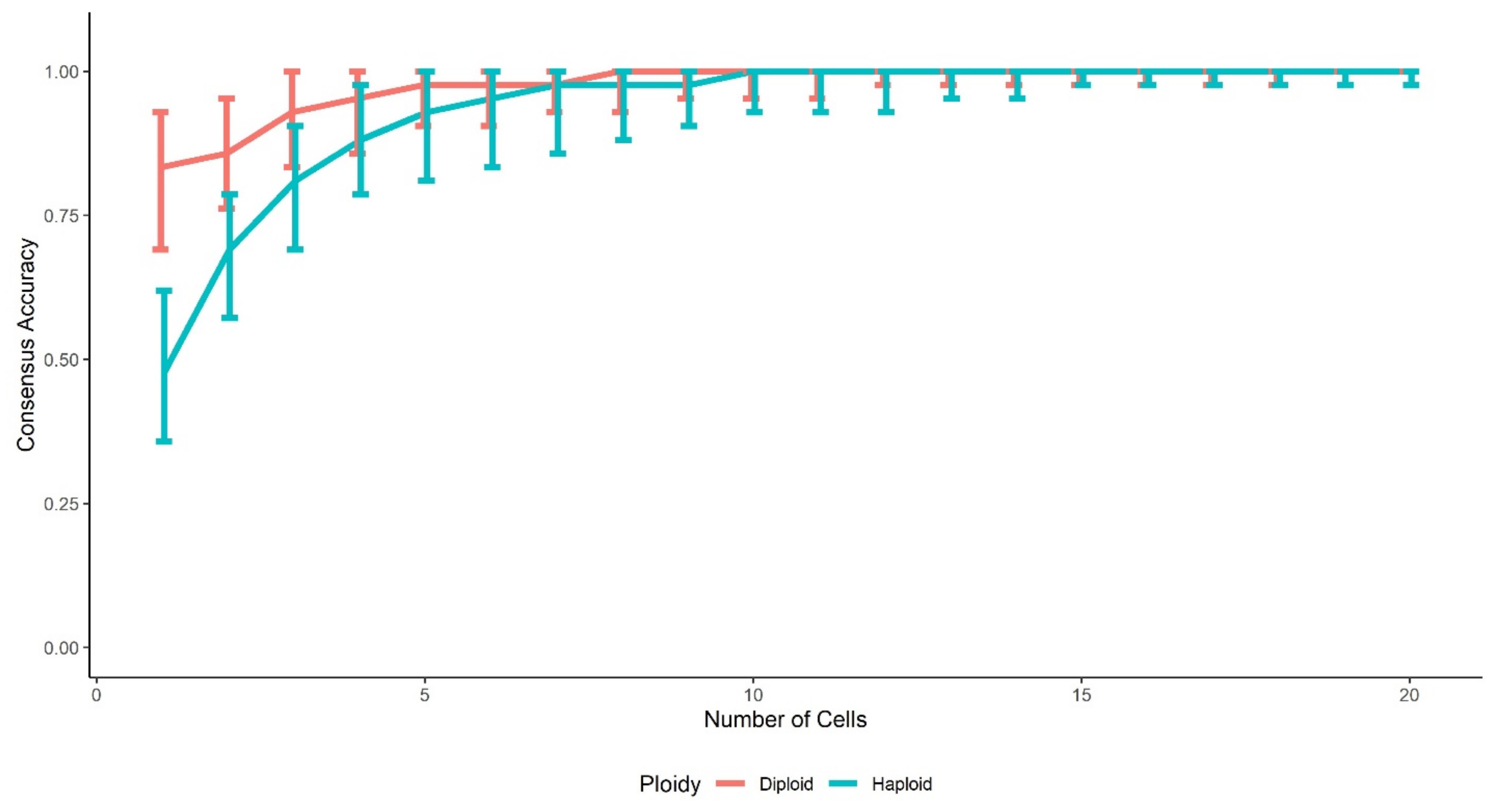
3.3. Accuracies of Consensus
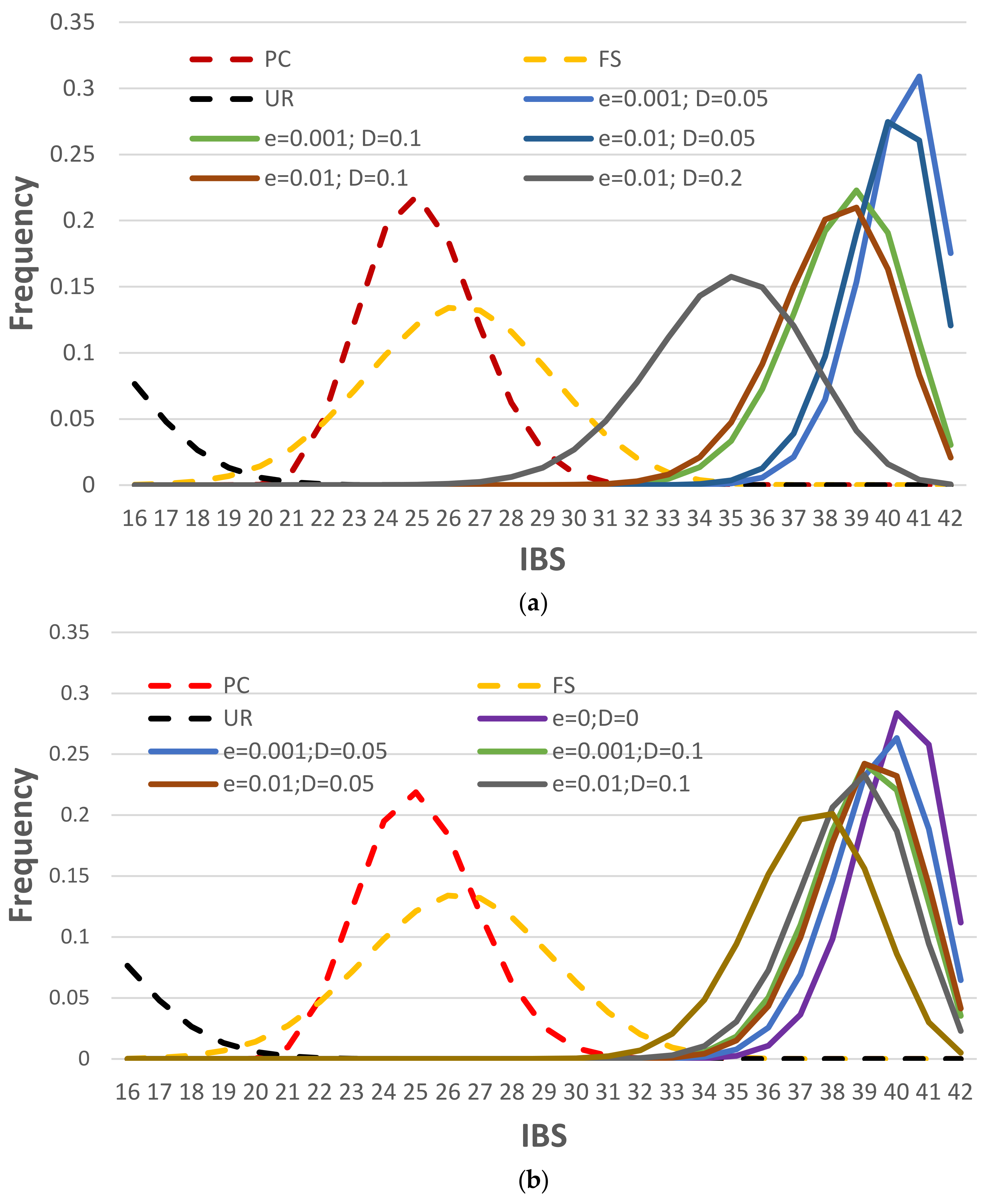
3.3.1. IBS Distributions with Consensus
3.3.2. A Suspect or His/Her Close Relatives as Contributors
3.3.3. Accuracies of Consensus by Clustering
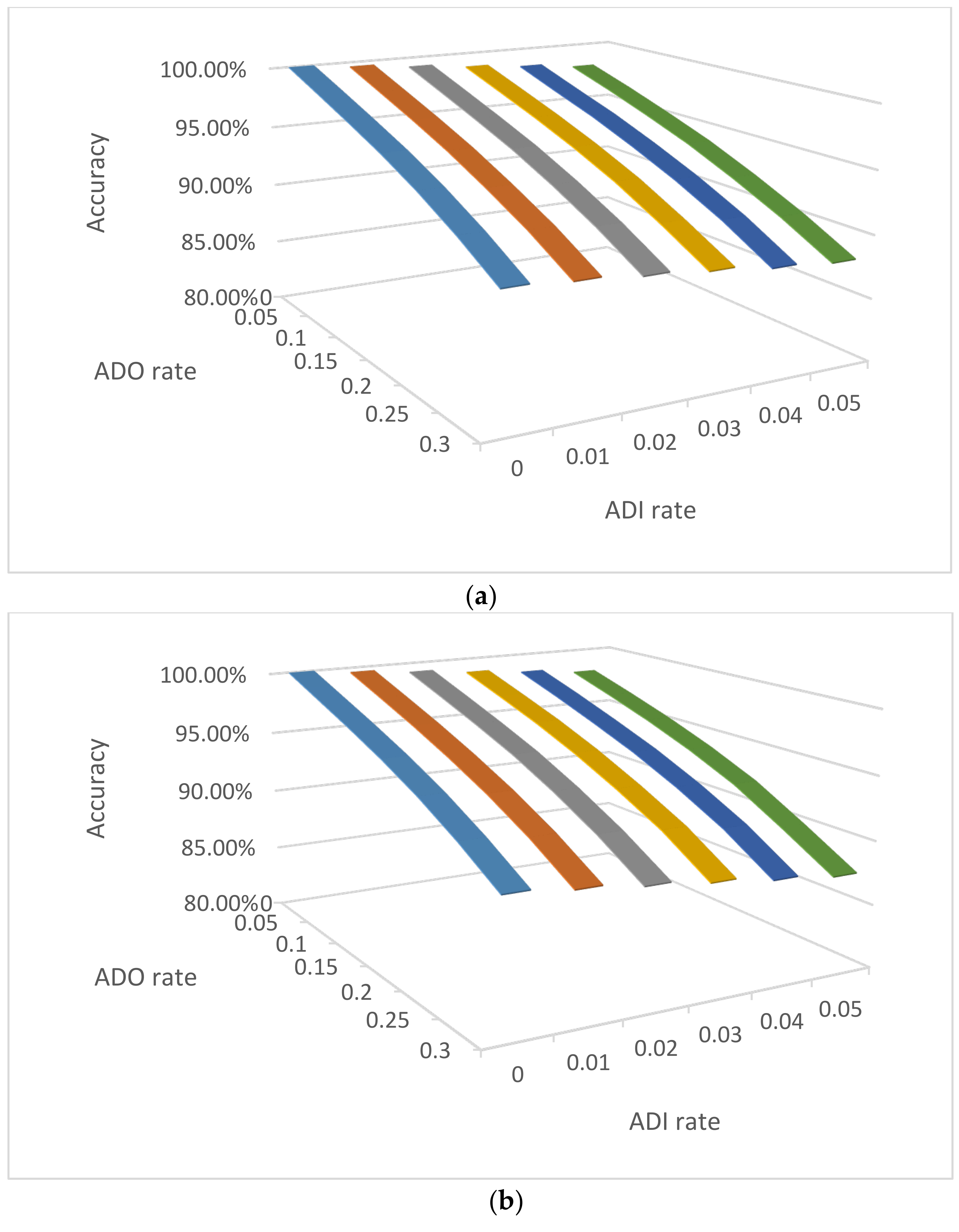
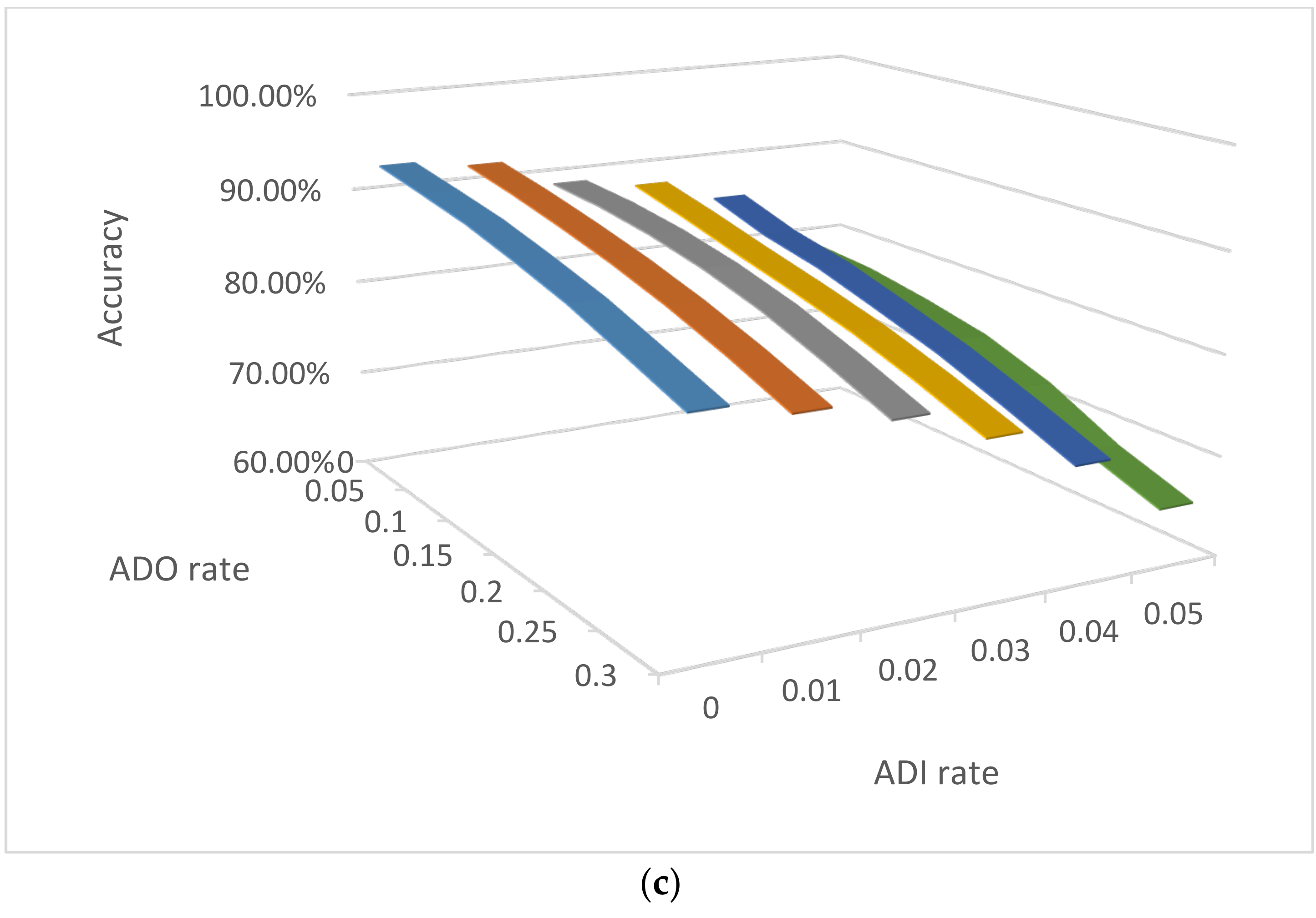
3.3.4. Impact of ADO and ADI on Consensus Accuracies
4. Discussion
4.1. A Paradigm Shift of Mixture Interpretation
4.2. The Capabilities and Limitations
4.3. Future Improvements
4.4. Costs
5. Conclusions
Supplementary Materials
Author Contributions
Funding
Institutional Review Board Statement
Informed Consent Statement
Data Availability Statement
Conflicts of Interest
References
- Bright, J.-A.; Taylor, D.; McGovern, C.; Cooper, S.; Russell, L.; Abarno, D.; Buckleton, J. Developmental validation of STRmix™, expert software for the interpretation of forensic DNA profiles. Forensic Sci. Int. Genet. 2016, 23, 226–239. [Google Scholar] [CrossRef] [PubMed]
- Gill, P.; Haned, H.; Eduardoff, M.; Santos, C.; Phillips, C.; Parson, W. The open-source software LRmix can be used to analyse SNP mixtures. Forensic Sci. Int. Genet. Suppl. Ser. 2015, 5, e50–e51. [Google Scholar] [CrossRef] [Green Version]
- Perlin, M.W.; Legler, M.M.; Spencer, C.E.; Smith, J.L.; Allan, W.P.; Belrose, J.L.; Duceman, B.W. Validating TrueAllele DNA mixture interpretation. J. Forensic Sci. 2011, 56, 1430–1447. [Google Scholar] [CrossRef]
- Gill, P.; Jeffreys, A.J.; Werrett, D.J. Forensic application of DNA ‘fingerprints’. Nature 1985, 318, 577–579. [Google Scholar] [CrossRef] [PubMed]
- Voorhees, J.C.; Ferrance, J.P.; Landers, J.P. Enhanced elution of sperm from cotton swabs via. enzymatic digestion for rape kit analysis. J. Forensic Sci. 2006, 51, 574–579. [Google Scholar] [CrossRef] [PubMed]
- Novroski, N.M.; King, J.L.; Churchill, J.D.; Seah, L.H.; Budowle, B. Characterization of genetic sequence variation of 58 STR loci in four major population groups. Forensic Sci. Int. Genet. 2016, 25, 214–226. [Google Scholar] [CrossRef] [PubMed]
- Gan, Y.; Li, N.; Zou, G.; Xin, Y.; Guan, J. Identification of cancer subtypes from single-cell RNA-seq data using a consensus clustering method. BMC Med. Genom. 2018, 11, 117. [Google Scholar] [CrossRef]
- Cui, Y.; Zhang, S.; Liang, Y.; Wang, X.; Ferraro, T.N.; Chen, Y. Consensus clustering of single-cell RNA-seq data by enhancing network affinity. Brief. Bioinform. 2021, bbab236. [Google Scholar] [CrossRef]
- Kling, D.; Tillmar, A.O.; Egeland, T. Familias 3-extensions and new functionality. Forensic Sci. Int. Genet. 2014, 13, 121–127. [Google Scholar] [CrossRef] [PubMed]
- Vullo, C.M.; Catelli, L.; Rodriguez, A.A.I.; Papaioannou, A.; Merino, J.C.Á.; Lopez-Parra, A.; Gaviria, A.; Baeza-Richer, C.; Romanini, C.; González-Moya, E. Second GHEP-ISFG exercise for DVI: “DNA-led” victims’ identification in a simulated air crash. Forensic Sci. Int. Genet. 2021, 53, 102527. [Google Scholar] [CrossRef]
- Budowle, B.; Eisenberg, A.J.; Van Daal, A. Validity of low copy number typing and applications to forensic science. Croat. Med. J. 2009, 50, 207–217. [Google Scholar] [CrossRef]
- Li, C.; Qi, B.; Ji, A.; Xu, X.; Hu, L. The combination of single cell micromanipulation with LV-PCR system and its application in forensic science. Forensic Sci. Int. Genet. Suppl. Ser. 2009, 2, 516–517. [Google Scholar] [CrossRef]
- Huffman, K.; Hanson, E.; Ballantyne, J. Recovery of single source DNA profiles from mixtures by direct single cell subsampling and simplified micromanipulation. Sci. Justice 2021, 61, 13–25. [Google Scholar] [CrossRef] [PubMed]
- Xu, C.; Feng, L.; Yang, F.; Jia, J.; Ji, A.-Q.; Hu, L.; Li, C.-X. Mucosal cell isolation and analysis from cellular mixtures of three contributors. J. Forensic Sci. 2015, 60, 783–786. [Google Scholar] [CrossRef] [PubMed]
- Brück, S.; Evers, H.; Heidorn, F.; Müller, U.; Kilper, R.; Verhoff, M.A. Single cells for forensic DNA analysis-from evidence material to test tube. J. Forensic Sci. 2010, 56, 176–180. [Google Scholar] [CrossRef] [PubMed]
- Schneider, C.; Müller, U.; Kilper, R.; Siebertz, B. Low copy number DNA profiling from isolated sperm using the aureka®-micromanipulation system. Forensic Sci. Int. Genet. 2012, 6, 461–465. [Google Scholar] [CrossRef] [PubMed]
- Theunissen, G.M.; Rolf, B.; Gibb, A.; Jäger, R. DNA profiling of sperm cells by using micromanipulation and whole genome amplification. Forensic Sci. Int. Genet. Suppl. Ser. 2017, 6, e497–e499. [Google Scholar] [CrossRef] [Green Version]
- Vandewoestyne, M.; Deforce, D. Laser capture microdissection in forensic research: A review. Int. J. Leg. Med. 2010, 124, 513–521. [Google Scholar] [CrossRef] [PubMed] [Green Version]
- Han, J.-P.; Yang, F.; Xu, C.; Wei, Y.-L.; Zhao, X.-C.; Hu, L.; Ye, J.; Li, C.-X. A new strategy for sperm isolation and STR typing from multi-donor sperm mixtures. Forensic Sci. Int. Genet. 2014, 13, 239–246. [Google Scholar] [CrossRef]
- Xu, Y.; Xie, J.; Chen, R.; Cao, Y.; Ping, Y.; Xu, Q.; Hu, W.; Wu, D.; Gu, L.; Zhou, H.; et al. Fluorescence- and magnetic-activated cell sorting strategies to separate spermatozoa involving plural contributors from biological mixtures for human identification. Sci. Rep. 2016, 6, 36515. [Google Scholar] [CrossRef] [PubMed] [Green Version]
- Schoell, W.M. Separation of sperm and vaginal cells with flow cytometry for DNA typing after sexual assault. Obstet. Gynecol. 1999, 94, 623–627. [Google Scholar] [CrossRef]
- Verdon, T.J.; Mitchell, R.J.; Chen, W.; Xiao, K.; van Oorschot, R.A. FACS separation of non-compromised forensically relevant biological mixtures. Forensic Sci. Int. Genet. 2015, 14, 194–200. [Google Scholar] [CrossRef]
- Miller, J.M.; Brocato, E.R.; Yadavalli, V.K.; Greenspoon, S.A.; Ehrhardt, C.J. Testing hormone-specific antibody probes for presumptive detection and separation of contributor cell populations in trace DNA mixtures. bioRxiv 2019. [Google Scholar] [CrossRef]
- Stokes, N.A.; Stanciu, C.E.; Brocato, E.R.; Ehrhardt, C.J.; Greenspoon, S.A. Simplification of complex DNA profiles using front end cell separation and probabilistic modeling. Forensic Sci. Int. Genet. 2018, 36, 205–212. [Google Scholar] [CrossRef]
- Dean, L.; Kwon, Y.J.; Philpott, M.K.; Stanciu, C.E.; Seashols-Williams, S.J.; Cruz, T.D.; Sturgill, J.; Ehrhardt, C.J. Separation of uncompromised whole blood mixtures for single source STR profiling using fluorescently-labeled human leukocyte antigen (HLA) probes and fluorescence activated cell sorting (FACS). Forensic Sci. Int. Genet. 2015, 17, 8–16. [Google Scholar] [CrossRef] [PubMed]
- Williamson, V.R.; Laris, T.M.; Romano, R.; Marciano, M.A. Enhanced DNA mixture deconvolution of sexual offense samples using the DEPArray™ system. Forensic Sci. Int. Genet. 2018, 34, 265–276. [Google Scholar] [CrossRef] [Green Version]
- Anslinger, K.; Graw, M.; Bayer, B. Deconvolution of blood-blood mixtures using DEPArrayTM separated single cell STR profiling. Rechtsmedizin 2019, 29, 30–40. [Google Scholar] [CrossRef] [Green Version]
- Fontana, F.; Rapone, C.; Bregola, G.; Aversa, R.; de Meo, A.; Signorini, G.; Sergio, M.; Ferrarini, A.; Lanzellotto, R.; Medoro, G.; et al. Isolation and genetic analysis of pure cells from forensic biological mixtures: The precision of a digital approach. Forensic Sci. Int. Genet. 2017, 29, 225–241. [Google Scholar] [CrossRef] [PubMed] [Green Version]
- England, R.; Nancollis, G.; Stacey, J.; Sarman, A.; Min, J.; Harbison, S. Compatibility of the ForenSeq™ DNA signature prep kit with laser microdissected cells: An exploration of issues that arise with samples containing low cell numbers. Forensic Sci. Int. Genet. 2020, 47, 102278. [Google Scholar] [CrossRef]
- Lim, H.H.; Srisiri, K.; Rerkamnuaychoke, B.; Bandhaya, A. A comparative study of whole genome amplification and low-template DNA profiling. Forensic Sci. Int. Genet. Suppl. Ser. 2019, 7, 509–511. [Google Scholar] [CrossRef]
- Deleye, L.; Plaetsen, A.-S.V.; Weymaere, J.; Deforce, D.; Van Nieuwerburgh, F. Short tandem repeat analysis after whole genome amplification of single B-lymphoblastoid cells. Sci. Rep. 2018, 8, 1–6. [Google Scholar] [CrossRef] [Green Version]
- Schneider, P.; Balogh, K.; Naveran, N.; Bogus, M.; Bender, K.; Lareu, M.; Carracedo, A. Whole genome amplification—the solution for a common problem in forensic casework? Int. Congr. Ser. 2004, 1261, 24–26. [Google Scholar] [CrossRef]
- Chen, M.; Zhang, J.; Zhao, J.; Chen, T.; Liu, Z.; Cheng, F.; Fan, Q.; Yan, J. Comparison of CE- and MPS-based analyses of forensic markers in a single cell after whole genome amplification. Forensic Sci. Int. Genet. 2020, 45, 102211. [Google Scholar] [CrossRef]
- Li, C.-X.; Han, J.-P.; Ren, W.-Y.; Ji, A.-Q.; Xu, X.-L.; Hu, L. DNA profiling of spermatozoa by laser capture microdissection and low volume-PCR. PLoS ONE 2011, 6, e22316. [Google Scholar] [CrossRef] [PubMed]
- Chen, C.; Xing, D.; Tan, L.; Li, H.; Zhou, G.; Huang, L.; Xie, X.S. Single-cell whole-genome analyses by linear amplification via. transposon insertion (LIANTI). Science 2017, 356, 189–194. [Google Scholar] [CrossRef] [PubMed] [Green Version]
- Ge, J.; Budowle, B.; Chakraborty, R. Choosing relatives for DNA identification of missing persons. J. Forensic Sci. 2011, 56, S23–S28. [Google Scholar] [CrossRef] [PubMed]
- Ge, J.; Budowle, B. Kinship index variations among populations and thresholds for familial searching. PLoS ONE 2012, 7, e37474. [Google Scholar] [CrossRef] [PubMed]
- Balding, D.J.; Nichols, R.A. DNA profile match probability calculation: How to allow for population stratification, relatedness, database selection and single bands. Forensic Sci. Int. 1994, 64, 125–140. [Google Scholar] [CrossRef]
- Ge, J.; Budowle, B.; Chakraborty, R. DNA identification by pedigree likelihood ratio accommodating population substructure and mutations. Investig. Genet. 2010, 1, 8. [Google Scholar] [CrossRef] [Green Version]
- AABB. Relationship Testing Annual Reports; AABB: Bethesda, MD, USA, 2008. [Google Scholar]
- Wang, D.Y.; Gopinath, S.; Lagacé, R.E.; Norona, W.; Hennessy, L.K.; Short, M.L.; Mulero, J.J. Developmental validation of the GlobalFiler® express PCR amplification kit: A 6-dye multiplex assay for the direct amplification of reference samples. Forensic Sci. Int. Genet. 2015, 19, 148–155. [Google Scholar] [CrossRef]
- Moretti, T.R.; Moreno, L.I.; Smerick, J.B.; Pignone, M.L.; Hizon, R.; Buckleton, J.S.; Bright, J.-A.; Onorato, A.J. Population data on the expanded CODIS core STR loci for eleven populations of significance for forensic DNA analyses in the United States. Forensic Sci. Int. Genet. 2016, 25, 175–181. [Google Scholar] [CrossRef] [Green Version]
- Eibe, F.; Hall, M.A.; Witten, I.H. Online Appendix for Data Mining: Practical Machine Learning Tools and Techniques; The WEKA Workbench; Morgan Kaufmann: Burlington, MA, USA, 2016. [Google Scholar]
- Balding, D.J.; Buckleton, J. Interpreting low template DNA profiles. Forensic Sci. Int. Genet. 2009, 4, 1–10. [Google Scholar] [CrossRef]
- Dempster, A.P.; Laird, N.M.; Rubin, D.B. Maximum likelihood from incomplete data via the EM algorithm. J. R. Stat. Soc. Ser. B 1977, 39, 1–22. [Google Scholar]
- Witten, I.H.; Frank, E.; Hall, M.A. Data Mining: Practical Machine Learning Tools and Techniques, 3rd ed.; Elsevier/Morgan Kaufmann: San Francisco, CA, USA, 2011. [Google Scholar] [CrossRef] [Green Version]
- Kanungo, T.; Mount, D.; Netanyahu, N.; Piatko, C.; Silverman, R.; Wu, A. An efficient k-means clustering algorithm: Analysis and implementation. IEEE Trans. Pattern Anal. Mach. Intell. 2002, 24, 881–892. [Google Scholar] [CrossRef]
- Rousseeuw, P.J. Silhouettes: A graphical aid to the interpretation and validation of cluster analysis. J. Comput. Appl. Math. 1987, 20, 53–65. [Google Scholar] [CrossRef] [Green Version]
- Morris, J.H.; Apeltsin, L.; Newman, A.M.; Baumbach, J.; Wittkop, T.; Su, G.; Bader, G.D.; Ferrin, T.E. ClusterMaker: A multi-algorithm clustering plugin for cytoscape. BMC Bioinform. 2011, 12, 436. [Google Scholar] [CrossRef] [Green Version]
- Kaufman, L.; Rousseeuw, P.J. Finding Groups in Data: An Introduction to Cluster Analysis; John Wiley and Sons: Hoboken, NJ, USA, 2009. [Google Scholar]
- Pich, C. MDSJ: Java Library for Multidimensional Scaling (Version 0.2). 2009. Available online: http://www.inf.uni-konstanz.de/algo/software/mdsj (accessed on 21 October 2020).
- Java Data Frame and Visualization Library. Available online: https://jtablesaw.github.io/tablesaw/ (accessed on 21 October 2020).
- Cairns, P. Gene methylation and early detection of genitourinary cancer: The road ahead. Nat. Rev. Cancer 2007, 7, 531–543. [Google Scholar] [CrossRef] [PubMed]
- Xuan, L.; Zhigang, C.; Fan, Y. Exploring of clustering algorithm on class-imbalanced data. In Proceedings of the 2013 8th International Conference on Computer Science & Education, Colombo, Sri Lanka, 26–28 April 2013; pp. 89–93. [Google Scholar]
- Wang, B.; Zhu, J.; Pierson, E.; Ramazzotti, D.; Batzoglou, S. Visualization and analysis of single-cell RNA-seq data by kernel-based similarity learning. Nat. Methods 2017, 14, 414–416. [Google Scholar] [CrossRef]
- Amir, E.-A.D.; Davis, K.L.; Tadmor, M.D.; Simonds, E.; Levine, J.H.; Bendall, S.C.; Shenfeld, D.K.; Krishnaswamy, S.; Nolan, G.P.; Pe’Er, D. ViSNE enables visualization of high dimensional single-cell data and reveals phenotypic heterogeneity of leukemia. Nat. Biotechnol. 2013, 31, 545–552. [Google Scholar] [CrossRef] [PubMed] [Green Version]
- Lucy, D.; Curran, J.; Pirie, A.; Gill, P. The probability of achieving full allelic representation for LCN-STR profiling of haploid cells. Sci. Justice 2007, 47, 168–171. [Google Scholar] [CrossRef] [PubMed]
- Council, N.R. An Update: The Evaluation of Forensic DNA Evidence; National Academies Press: Washington, DC, USA, 1996. [Google Scholar]
- Wall, J.D.; Tang, L.F.; Zerbe, B.; Kvale, M.N.; Kwok, P.-Y.; Schaefer, C.; Risch, N. Estimating genotype error rates from high-coverage next-generation sequence data. Genome Res. 2014, 24, 1734–1739. [Google Scholar] [CrossRef] [PubMed] [Green Version]
- Ge, J.; Budowle, B. Modeling one complete versus triplicate analyses in low template DNA typing. Int. J. Leg. Med. 2013, 128, 259–267. [Google Scholar] [CrossRef] [PubMed]
- Ge, J.; Chakraborty, R.; Eisenberg, A.; Budowle, B. Comparisons of familial DNA database searching strategies. J. Forensic Sci. 2011, 56, 1448–1456. [Google Scholar] [CrossRef] [PubMed]
- Kobak, D.; Berens, P. The art of using t-SNE for single-cell transcriptomics. Nat. Commun. 2019, 10, 1–14. [Google Scholar] [CrossRef] [Green Version]
- Chen, L.; He, Q.; Zhai, Y.; Deng, M. Single-cell RNA-seq data semi-supervised clustering and annotation via. structural regularized domain adaptation. Bioinformatics 2021, 37, 775–784. [Google Scholar] [CrossRef]
- Chen, L.; Zhai, Y.; He, Q.; Wang, W.; Deng, M. Integrating deep supervised, self-supervised and unsupervised learning for single-cell RNA-seq clustering and annotation. Genes 2020, 11, 792. [Google Scholar] [CrossRef]
- Lin, M.-H.; Bright, J.-A.; Pugh, S.N.; Buckleton, J.S. The interpretation of mixed DNA profiles from a mother, father, and child trio. Forensic Sci. Int. Genet. 2020, 44, 102175. [Google Scholar] [CrossRef] [Green Version]
- Stoeckius, M.; Zheng, S.; Houck-Loomis, B.; Hao, S.; Yeung, B.Z.; Mauck, W.M.; Smibert, P.; Satija, R. Cell hashing with barcoded antibodies enables multiplexing and doublet detection for single cell genomics. Genome Biol. 2018, 19, 1–12. [Google Scholar] [CrossRef] [Green Version]
- Zhang, L.; Dong, X.; Lee, M.; Maslov, A.Y.; Wang, T.; Vijg, J. Single-cell whole-genome sequencing reveals the functional landscape of somatic mutations in B lymphocytes across the human lifespan. Proc. Natl. Acad. Sci. USA 2019, 116, 9014–9019. [Google Scholar] [CrossRef] [Green Version]
- Woerner, A.E.; Mandape, S.; King, J.L.; Muenzler, M.; Crysup, B.; Budowle, B. Reducing noise and stutter in short tandem repeat loci with unique molecular identifiers. Forensic Sci. Int. Genet. 2021, 51, 102459. [Google Scholar] [CrossRef]
- Sheth, N.; Swaminathan, H.; Gonzalez, A.J.; Duffy, K.R.; Grgicak, C.M. Towards developing forensically relevant single-cell pipelines by incorporating direct-to-PCR extraction: Compatibility, signal quality, and allele detection. Int. J. Leg. Med. 2021, 135, 727–738. [Google Scholar] [CrossRef] [PubMed]
- Lin, W.-C.; Tsai, C.-F.; Hu, Y.-H.; Jhang, J.-S. Clustering-based undersampling in class-imbalanced data. Inf. Sci. 2017, 409-410, 17–26. [Google Scholar] [CrossRef]
- Liu, F.T.; Ting, K.M.; Zhou, Z.-H. Isolation forest. In Proceedings of the 2008 Eighth IEEE International Conference on Data Mining, Washington, DC, USA, 15–19 December 2008; pp. 413–422. [Google Scholar]
- Yang, Y.; Xu, Z. Rethinking the value of labels for improving class-imbalanced learning. arXiv 2006, arXiv:2006.07529 2020. [Google Scholar]


| No. of Cells | 2-Person Mixture | 3-Person Mixture | |||||||||
|---|---|---|---|---|---|---|---|---|---|---|---|
| Mixture | Diploid | Haploid | Mixture | Diploid | Haploid | ||||||
| UR | PC | FS | UR | PC | FS | UR | Trio | UR | |||
| 160 | 80,80 | 100.00% | 100.00% | 99.90% | 99.90% | 98.04% | 92.16% | 53,53,53 | 99.96% | 88.32% | 96.55% |
| 106,54 | 100.00% | 99.98% | 99.74% | 99.88% | 96.53% | 89.27% | 32,32,96 | 99.69% | 85.64% | 81.79% | |
| 128,32 | 100.00% | 99.85% | 98.87% | 99.16% | 91.35% | 81.70% | 16,48,96 | 98.60% | 78.46% | 52.55% | |
| 144,16 | 99.97% | 98.54% | 94.86% | 95.97% | 87.64% | 81.28% | |||||
| 152,8 | 99.55% | 91.59% | 86.12% | 92.43% | 87.98% | 83.97% | |||||
| 80 | 40,40 | 100.00% | 99.93% | 99.91% | 99.93% | 98.73% | 96.32% | 26,26,26 | 99.97% | 87.94% | 96.44% |
| 53,27 | 100.00% | 99.94% | 99.78% | 99.87% | 98.17% | 94.40% | 16,16,48 | 99.68% | 86.51% | 82.47% | |
| 64,16 | 99.99% | 99.96% | 99.53% | 99.71% | 94.37% | 87.68% | 8,24,48 | 98.36% | 80.54% | 54.15% | |
| 72,8 | 99.96% | 98.99% | 96.55% | 95.56% | 85.95% | 81.09% | |||||
| 76,4 | 99.67% | 93.47% | 88.56% | 88.91% | 83.54% | 79.10% | |||||
| 40 | 20,20 | 100.00% | 99.99% | 99.93% | 99.72% | 95.25% | 92.41% | 13,13,13 | 99.96% | 88.29% | 91.81% |
| 26,14 | 100.00% | 99.93% | 99.87% | 99.76% | 94.56% | 90.23% | 8,8,24 | 99.79% | 86.06% | 76.22% | |
| 32,8 | 100.00% | 99.89% | 99.22% | 99.18% | 89.52% | 81.95% | 4,12,24 | 98.44% | 79.79% | 46.55% | |
| 36,4 | 99.90% | 98.03% | 95.37% | 93.40% | 76.58% | 71.13% | |||||
| 38,2 | 95.49% | 78.98% | 74.69% | 84.31% | 68.47% | 65.89% | |||||
| 20 | 10,10 | 100.00% | 99.54% | 99.02% | 97.21% | 82.30% | 79.50% | 6,6,6 | 99.81% | 85.59% | 69.19% |
| 13,7 | 99.98% | 99.48% | 98.84% | 97.30% | 82.77% | 79.09% | 4,4,12 | 99.52% | 82.22% | 51.34% | |
| 16,4 | 99.96% | 99.62% | 98.92% | 95.34% | 73.85% | 70.30% | 2,6,12 | 89.80% | 72.16% | 21.69% | |
| 18,2 | 99.61% | 97.00% | 94.29% | 81.92% | 59.54% | 58.65% | |||||
| 19,1 | 98.51% | 86.74% | 82.46% | 60.82% | 53.45% | 53.40% | |||||
| 10 | 5,5 | 99.95% | 96.77% | 94.02% | 82.78% | 56.59% | 55.61% | 3,3,3 | 97.16% | 66.81% | 33.58% |
| 6,4 | 99.84% | 96.65% | 93.90% | 80.38% | 55.79% | 53.41% | 2,2,6 | 99.05% | 76.26% | 38.63% | |
| 8,2 | 99.68% | 94.61% | 91.60% | 78.59% | 49.60% | 48.24% | 1,3,6 | 59.31% | 37.65% | 12.44% | |
| 9,1 | 98.91% | 89.19% | 85.09% | 65.71% | 41.74% | 42.05% | |||||
| No. of Cells | DNA Quantity (pg) | The Mixture Proportion of a Contributor | |||||
|---|---|---|---|---|---|---|---|
| Diploid | Haploid | 1% | 5% | 10% | 20% | 50% | |
| 1 | 6.6 | 3.3 | 99.00% | 95.00% | 90.00% | 80.00% | 50.00% |
| 5 | 33 | 16.5 | 95.10% | 77.38% | 59.05% | 32.77% | 3.13% |
| 10 | 66 | 33 | 90.44% | 59.87% | 34.87% | 10.74% | 0.10% |
| 15 | 99 | 49.5 | 86.01% | 46.33% | 20.59% | 3.52% | 0.00% |
| 20 | 132 | 66 | 81.79% | 35.85% | 12.16% | 1.15% | 0.00% |
| 40 | 264 | 132 | 66.90% | 12.85% | 1.48% | 0.01% | 0.00% |
| 80 | 528 | 264 | 44.75% | 1.65% | 0.02% | 0.00% | 0.00% |
| 160 | 1056 | 528 | 20.03% | 0.03% | 0.00% | 0.00% | 0.00% |
| 500 | 3300 | 1650 | 0.66% | 0.00% | 0.00% | 0.00% | 0.00% |
| No. of Cells. | 2-Person Mixture | 3-Person Mixture | |||||||||
|---|---|---|---|---|---|---|---|---|---|---|---|
| Mixture | Diploid | Haploid | Mixture | Diploid | Haploid | ||||||
| UR | PC | FS | UR | PC | FS | UR | Trio | UR | |||
| 160 | 80,80 | 100.00% | 100.00% | 100.00% | 100.00% | 99.93% | 99.28% | 53,53,53 | 100.00% | 100.00% | 100.00% |
| 106,54 | 100.00% | 100.00% | 99.99% | 100.00% | 99.80% | 98.83% | 32,32,96 | 100.00% | 100.00% | 99.94% | |
| 128,32 | 100.00% | 99.98% | 99.90% | 99.55% | 98.64% | 97.17% | 16,48,96 | 99.96% | 99.95% | 99.47% | |
| 144,16 | 99.85% | 98.91% | 97.91% | 94.96% | 93.92% | 91.86% | |||||
| 152,8 | 98.01% | 90.16% | 89.05% | 81.77% | 85.70% | 84.88% | |||||
| 80 | 40,40 | 100.00% | 100.00% | 100.00% | 100.00% | 99.96% | 99.73% | 26,26,26 | 99.99% | 99.99% | 99.97% |
| 53,27 | 100.00% | 100.00% | 99.99% | 99.99% | 99.90% | 99.49% | 16,16,48 | 99.91% | 99.91% | 99.73% | |
| 64,16 | 99.94% | 99.93% | 99.89% | 99.75% | 99.09% | 97.90% | 8,24,48 | 99.47% | 99.45% | 98.53% | |
| 72,8 | 99.19% | 98.65% | 98.01% | 95.15% | 92.18% | 90.78% | |||||
| 76,4 | 96.40% | 93.09% | 91.63% | 81.77% | 83.45% | 83.02% | |||||
| 40 | 20,20 | 99.96% | 99.96% | 99.96% | 99.93% | 99.80% | 99.52% | 13,13,13 | 99.69% | 99.68% | 99.00% |
| 26,14 | 99.88% | 99.87% | 99.87% | 99.67% | 99.41% | 98.90% | 8,8,24 | 98.94% | 98.95% | 97.56% | |
| 32,8 | 99.21% | 99.18% | 99.08% | 98.37% | 96.61% | 95.43% | 4,12,24 | 97.79% | 97.78% | 94.55% | |
| 36,4 | 96.79% | 96.17% | 95.85% | 91.16% | 87.64% | 86.57% | |||||
| 38,2 | 85.79% | 81.23% | 81.22% | 76.48% | 78.91% | 78.88% | |||||
| 20 | 10,10 | 99.16% | 99.17% | 99.13% | 98.20% | 96.75% | 95.68% | 6,6,6 | 96.98% | 96.97% | 92.68% |
| 13,7 | 98.90% | 98.87% | 98.85% | 97.53% | 95.57% | 94.51% | 4,4,12 | 95.72% | 95.71% | 89.05% | |
| 16,4 | 96.83% | 96.80% | 96.71% | 93.02% | 89.51% | 88.51% | 2,6,12 | 94.02% | 94.02% | 84.83% | |
| 18,2 | 92.78% | 92.31% | 92.01% | 81.99% | 77.81% | 78.35% | |||||
| 19,1 | 90.85% | 88.80% | 87.86% | 69.30% | 68.57% | 69.78% | |||||
| 10 | 5,5 | 96.33% | 96.34% | 96.30% | 91.56% | 87.57% | 86.61% | 3,3,3 | 92.68% | 92.74% | 78.80% |
| 6,4 | 95.37% | 95.33% | 95.33% | 90.70% | 86.72% | 85.95% | 2,2,6 | 89.45% | 89.47% | 75.58% | |
| 8,2 | 92.11% | 91.99% | 91.97% | 82.58% | 78.46% | 77.78% | 1,3,6 | 90.86% | 90.42% | 66.12% | |
| 9,1 | 90.81% | 90.36% | 90.17% | 71.50% | 67.26% | 67.31% | |||||
Publisher’s Note: MDPI stays neutral with regard to jurisdictional claims in published maps and institutional affiliations. |
© 2021 by the authors. Licensee MDPI, Basel, Switzerland. This article is an open access article distributed under the terms and conditions of the Creative Commons Attribution (CC BY) license (https://creativecommons.org/licenses/by/4.0/).
Share and Cite
Ge, J.; King, J.L.; Smuts, A.; Budowle, B. Precision DNA Mixture Interpretation with Single-Cell Profiling. Genes 2021, 12, 1649. https://doi.org/10.3390/genes12111649
Ge J, King JL, Smuts A, Budowle B. Precision DNA Mixture Interpretation with Single-Cell Profiling. Genes. 2021; 12(11):1649. https://doi.org/10.3390/genes12111649
Chicago/Turabian StyleGe, Jianye, Jonathan L. King, Amy Smuts, and Bruce Budowle. 2021. "Precision DNA Mixture Interpretation with Single-Cell Profiling" Genes 12, no. 11: 1649. https://doi.org/10.3390/genes12111649
APA StyleGe, J., King, J. L., Smuts, A., & Budowle, B. (2021). Precision DNA Mixture Interpretation with Single-Cell Profiling. Genes, 12(11), 1649. https://doi.org/10.3390/genes12111649