Article

Estimates of Autozygosity Through Runs of Homozygosity in Farmed Coho Salmon

by
Grazyella M. Yoshida
1,
Pablo Cáceres
1,
Rodrigo Marín-Nahuelpi
1,
Ben F. Koop
2 and
José M. Yáñez
1,3,*
1
Facultad de Ciencias Veterinarias y Pecuarias, Universidad de Chile, Santiago 8820808, Chile
2
Department of Biology, Centre for Biomedical Research, University of Victoria, Victoria, BC V8W 2Y2, Canada
3
Nucleo Milenio INVASAL, Concepción 4030000, Chile
*
Author to whom correspondence should be addressed.
Genes 2020, 11(5), 490; https://doi.org/10.3390/genes11050490
Submission received: 3 April 2020 / Revised: 23 April 2020 / Accepted: 24 April 2020 / Published: 30 April 2020
(This article belongs to the Special Issue Genetics and Genomics of Salmonid Fishes)

Abstract

:
The characterization of runs of homozygosity (ROH), using high-density single nucleotide polymorphisms (SNPs) allows inferences to be made about the past demographic history of animal populations and the genomic ROH has become a common approach to characterize the inbreeding. We aimed to analyze and characterize ROH patterns and compare different genomic and pedigree-based methods to estimate the inbreeding coefficient in two pure lines (POP A and B) and one recently admixed line (POP C) of coho salmon (Oncorhynchus kisutch) breeding nuclei, genotyped using a 200 K Affymetrix Axiom® myDesign Custom SNP Array. A large number and greater mean length of ROH were found for the two “pure” lines and the recently admixed line (POP C) showed the lowest number and smaller mean length of ROH. The ROH analysis for different length classes suggests that all three coho salmon lines the genome is largely composed of a high number of short segments (<4 Mb), and for POP C no segment >16 Mb was found. A high variable number of ROH, mean length and inbreeding values across chromosomes; positively the consequence of artificial selection. Pedigree-based inbreeding values tended to underestimate genomic-based inbreeding levels, which in turn varied depending on the method used for estimation. The high positive correlations between different genomic-based inbreeding coefficients suggest that they are consistent and may be more accurate than pedigree-based methods, given that they capture information from past and more recent demographic events, even when there are no pedigree records available.

1. Introduction

Coho salmon (Oncorhynchus kisutch) is one of the six Pacific salmon species which can be found in North America and Asia [1]. In Chile, coho salmon farming was established during the late 1970s, date in which about a half of million eggs were imported from Oregon (USA) and the Kitimat river (British Columbia, Canada), giving origin to the basis of the commercial stocks in the country [2,3]. The first coho salmon breeding program started in 1992 with an increased growth rate as the main breeding objective. After four generations of selection for harvest weight, genetic gains of ~10% per generation were reported [2,3].
Genetic improvement programs for aquaculture species have been successfully established for increasing the productivity, for traits like growth and resistance against diseases [4,5]. However, one of the negative consequences of selective breeding is the accumulation of inbreeding, due to the use of related individuals for reproductive purposes [6]. As a consequence, a reduction in both the additive genetic variance and diversity is observed, as well as a decrease in the response to selection. Furthermore, inbreeding can result in inbreeding depression, defined as a reduction in fitness traits, including growth, survival and reproductive ability, due to the expression of detrimental recessive alleles given the existence of highly homozygous animals in the population [6,7]. Thus, monitoring and managing the inbreeding levels is critical in the operation of genetic improvement programs [8,9,10].
Pedigree-based inbreeding (Fped) is traditionally estimated by calculating the probability that an individual inherits two alleles that are identical-by-descendent (IBD). When Fped is used, the founder animals in the pedigree are considered unrelated. This assumption fails to capture the actual relatedness among animals from the base population [11]. Thus, pedigrees errors and incomplete or missing information might lead to incorrect or biased inbreeding estimates [12]. Furthermore, Fped is computed as an average expectation (i.e., probabilities) and does not consider the stochastic nature of recombination during meiosis and the finite number of chromosomes [13]. The development of genomic technologies, including dense single nucleotide polymorphism (SNP) panels, creates opportunities to estimate inbreeding from genomic-based approaches, e.g., by using a genomic relationship matrix to infer identity-by-state (IBS) [14] or through ROH [15].
ROH is defined as continuous DNA segments that are homozygous in a particular individual [16], as a potential consequence of not random mating, demographic history of consanguineous mating due to parents transmitting identical haplotypes to their offspring [17]. Therefore, ROH may provide a good measure of individual genome-wide autozygosity, which is the homozygote status generated by IBD alleles, that resulted from genetic drift, population bottleneck, the mating of close relatives and selection [13,18]. Furthermore, the identification and characterization of ROH can provide insights into population history, structure and demographics over time, allowing to distinguish between recent and ancient inbreeding [19,20]. Long ROH segments are indicative of recent IBD (>16 Mb = three generations), whereas short segments suggest ancient inbreeding (1 Mb = 50 generations). The sum of all these segments is suggested to be an accurate estimate of the actual inbreeding level of an individual [21]. However, it also possible that not all small size ROH are due to IBD, but to identity-by-status (IBS) due to low recombination rates in specific regions of the genome, high linkage disequilibrium in non-related ancestors and genetic drift.
Inbreeding studies using genome-wide data were previously reported in humans [16,22,23], livestock [24,25,26,27,28], swine [29,30,31], sheep [32], goats [33] and river buffalo [34]. Several studies have shown that ROH provides a better measure of individual autozygosity at the genomic level and the possibility to identify specific IBD regions [16,27,35]. A recent study reported ROH patterns in rainbow trout populations to show the impact on selection on the genetic diversity in farmed stocks [36]. However, studies aimed to characterize ROH patterns and comparisons between coefficients of inbreeding using different approaches are scarce in aquaculture species, due to the need of deep and complete pedigree information and dense genomic information, which most of the time is insufficient. The objectives of this study were to identify and characterize the ROH patterns, and to compare inbreeding coefficients estimated using genomic and pedigree information in three farmed Chilean coho salmon populations.

2. Methods

2.1. Coho Salmon Populations and Genotypes

Two independent coho salmon populations, managed in two-year reproductive cycles (POP A and POP B) were used in this study and belong to the Pesquera Antares breeding program established in Chile in 1997. Both populations have undergone nine generations of selection for harvest body weight, since 1997 and 1998, POP A and B respectively. In addition, POP C is the progeny produced by mating sires from the seventh and dams from eighth generations of POP A and B, respectively. POP C was generated in 2013 to limit inbreeding levels, as suggested by Yáñez et al. [8]. The reproduction system, fish tagging and selection criteria of coho salmon populations were described previously [37,38].
Genomic DNA was extracted from fin clips of 88, 45 and 104 animals from POP A, B and C, respectively. The samples were genotyped using a 200 K Affymetrix Axiom® myDesign Custom SNP Array developed by the EPIC4 coho salmon genome consortium (http://www.epic-4.org) and built by ThermoFisher Scientific (San Diego, CA, USA) [39]. A genotype quality control was performed in Plink v1.09 [40] using the following parameters to exclude markers: Hardy–Weinberg Equilibrium (HWE) p-value < 1 × 10⁻⁶, Minor Allele Frequency (MAF) <0.01 and call rate <0.90 for genotypes and samples. Furthermore, we retained only the SNP markers that commonly segregated among the three populations. Sampling protocols were approved by the Animal Bioethics Committee from Universidad de Chile (No. 08-2015) and all raw genotypic data are available at Figshare public repository (10.6084/m9.figshare.11931963).

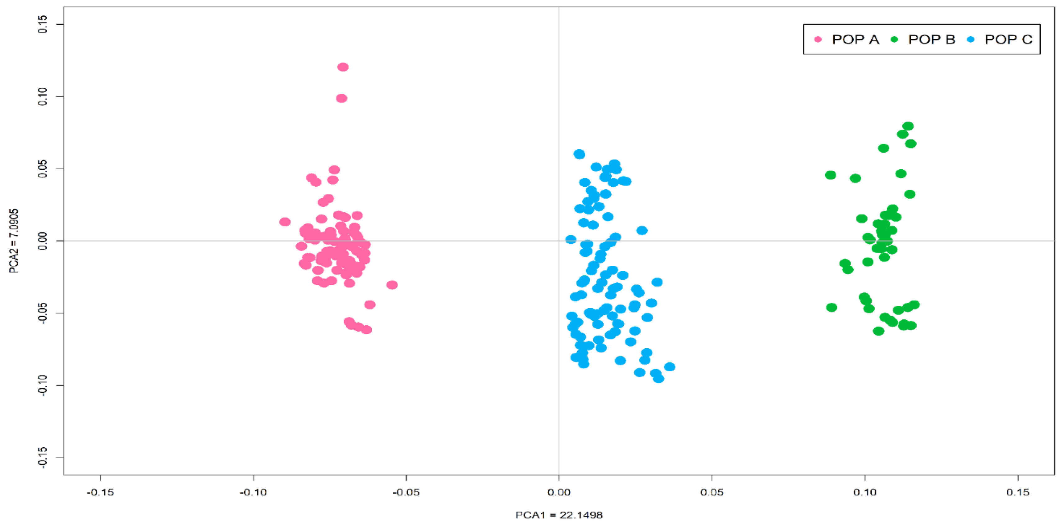
2.2. Principal Components and Admixture Analysis

We used the software Plink v1.09 [40] to evaluate the genetic differentiation among the three coho salmon populations through principal component analysis (PCA). The first two PCAs were plotted using R scripts [41]. The population structure was also examined using a hierarchical Bayesian model implemented in STRUCTURE software v.2.3.4 [42]. We used three replicates of K values ranging from 1 to 12, running of 50,000 iterations and burn-in of 20,000 iterations. To choose the best K value we used the statistic ΔK [43].

2.3. Runs of Homozygosity

Runs of homozygosity analysis was performed separately for all animals in each population using the R package detectRUNS [44]. The following constraints were applied to ROH detected: (i) the minimum number of SNPs included in an ROH was 50, (ii) the minimum length of an ROH was set at 1 Mb, (iii) the maximum distance between adjacent SNPs was 500 Kb, (iv) maximum missing genotypes allowed was 5, (v) density was at least 1 SNP per 50 kb and (vi) sliding windows approach was used to detect ROH for each genotyped animal at each marker position. ROH was classified into five-length classes: 1–2, 2–4, 4–8, 8–16 and >16 Mb, identified as ROH1–2 Mb, ROH2–4 Mb, ROH4–8 Mb, ROH8–16 Mb, and ROH>16 Mb, respectively.
Each ROH size class represent the number of generations from common ancestry, estimated as: E ( L I B D H | g c A ) = 100 2 g c A , where E ( L I B D H | g c A ) is the ROH segment length and gcA is the number of generations from the common ancestor [13]. Thus, we would expect that ROH1–2 Mb, ROH2–4 Mb, ROH4–8 Mb, ROH8–16 Mb, and ROH>16 Mb are dating to approximately 50, 20, 12.5, 6 and 3 generations ago by considering that the 1 cM equals 1 Mb.

2.4. Inbreeding Coefficient

We estimated inbreeding coefficients using three different genomic methods and pedigree relationship matrix (FPED). Inbreeding coefficient based on runs of homozygosity (FROH) was estimated for each animal based on all ROHs (ROHALL) and the ROH distribution of five different lengths (ROH1–2 Mb, ROH2–4 Mb, ROH4–8 Mb, ROH8–16 Mb, and ROH>16 Mb), as follows [16]:
F ROH = L R O H L A U T O ,
where LROH is the sum of ROH lengths and LAUTO is the total length of the genome covered by the genome-wide SNP panel used, assumed to be 1685.79 Mb.
The FHOM was calculated based on genome-wide homozygous excess due to inbreeding as follows [45]:
F HOM = O h o m E h o m N E h o m ,
where O h o m is the observed number of homozygous markers in each individual, E h o m is the expected number of homozygous markers under the Hardy-Weinberg equilibrium calculated from the allele frequencies estimated based on the sample and N is the total number of markers.
The FGRM was estimated using the genomic relationship matrix (GRM) [14], as follows:
G = Z Z 2 i = 1 n p i ( 1 p i ) ,
where Z is a genotype matrix that contains the 0–2p values for homozygotes, 1–2p for heterozygotes, and 2–2p for opposite homozygotes, p is the allele frequency of SNP i. The diagonal elements of the matrix G represent the relationship of the animal j with itself, thus, the genomic inbreeding coefficient is calculated as 2Gjj–1.
Pedigree-based inbreeding coefficients were estimated using the software INBUPGF90 [46]. The pedigree information used was provided by Pesquera Antares breeding program in Chile, for all animals born between 1998 and 2014, 1997 and 2013 and 1998 and 2013 for POP A, B and C respectively. Pearson correlation between genomic- and pedigree-based inbreeding coefficients were estimated within and across all populations using function cor.test in R [41].

3. Results

3.1. Quality Control and Genomic Population Structure

From an initial number of 135,500 markers, a total of 102,129 passed in the QC and were shared among the three populations. A number of ~30 K, 21 K and 18 K markers for POP A, B and C, respectively were removed, most of them due to MAF criteria. In addition, a number of markers ranging from 3.2 K to 14.9 K were removed to select only common markers segregating across all three populations (Supplementary File 1).
In the PCA analysis, the first two eigenvectors, together, accounted for 29.2% of the total genetic variation and revealed three stratified populations (Figure 1). PCA1 included 22.15% of the total genetic variation and generated the principal clusters to differentiate the three coho salmon populations, whereas PCA2 explained the variation present within each population.
The best K-value for admixture analysis was selected after performing several runs of MCMC for each K-value (ranging from 1 to 12), based on the statistic ΔK the best K-value was suggested to be K = 4. These results indicated that for few individuals of POP A and POP B the proportion of ancestry come from a single cluster (green and yellow, respectively), and most of animals shared a proportion of their genome with each other, probably due to the similar origin of the source populations. In addition, Supplementary File 2 indicate a higher admixture level for most of animals from POP C, due to the recent cross between POP A and B to generate this population.

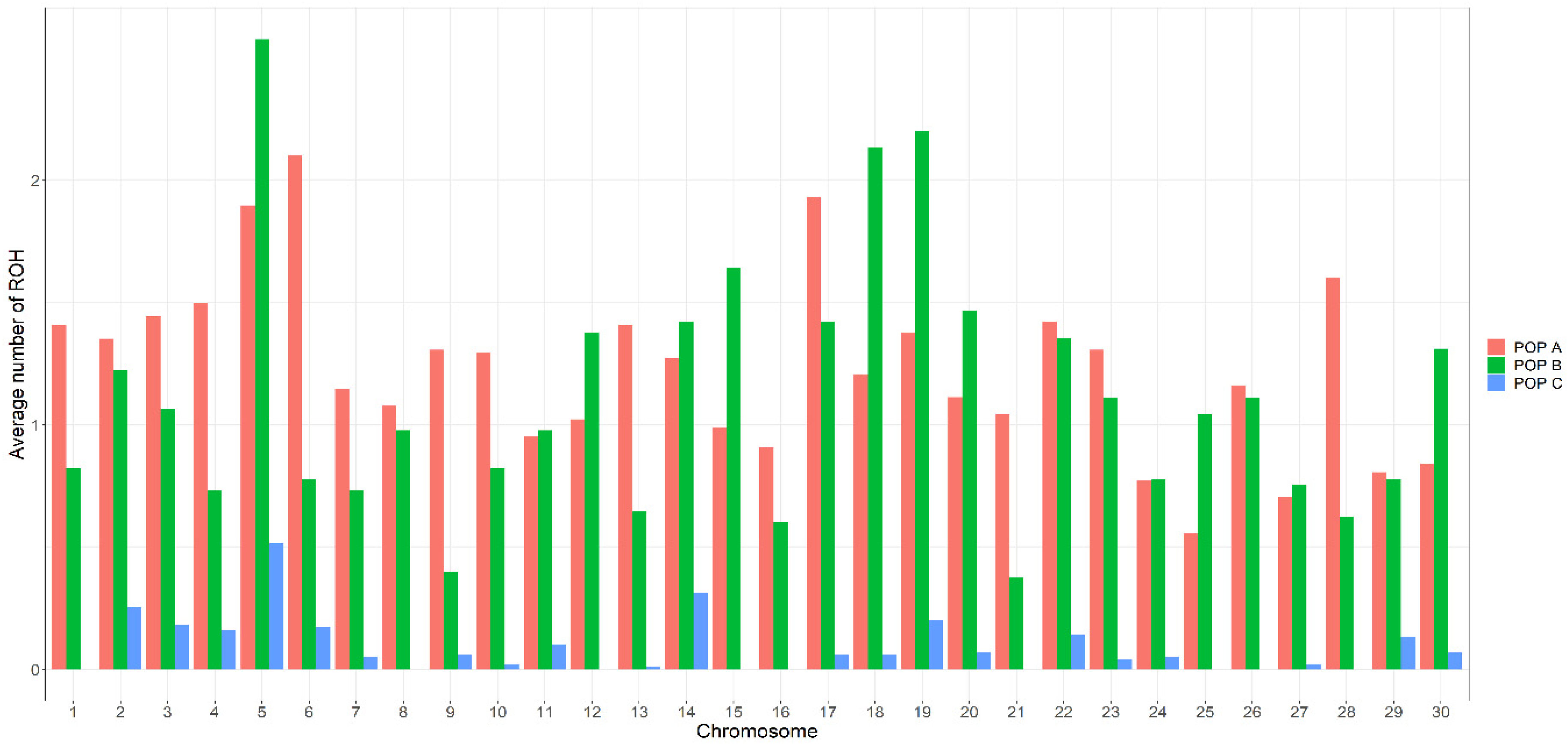
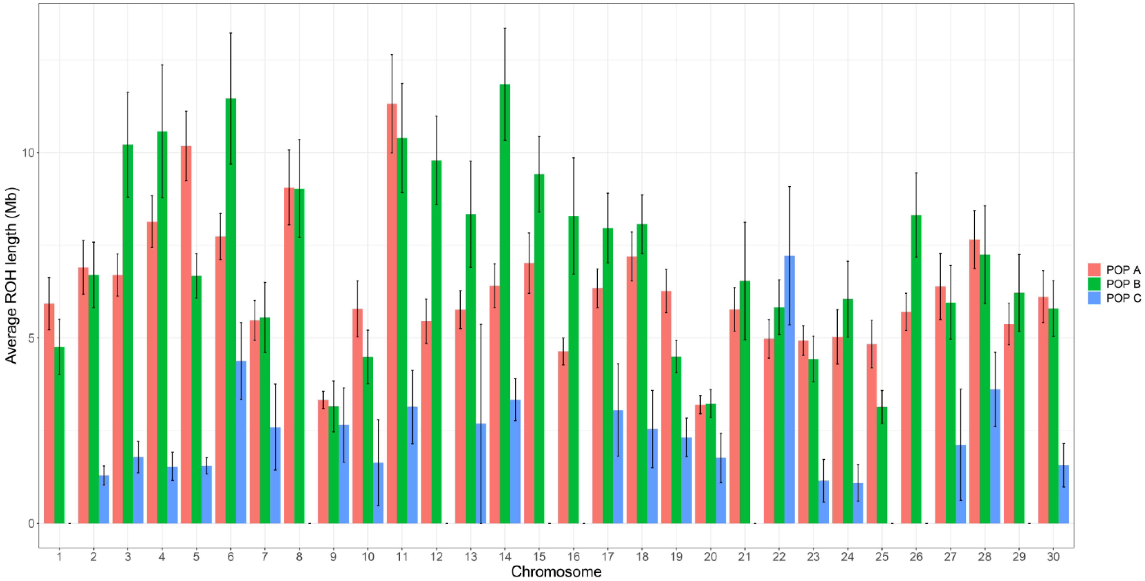
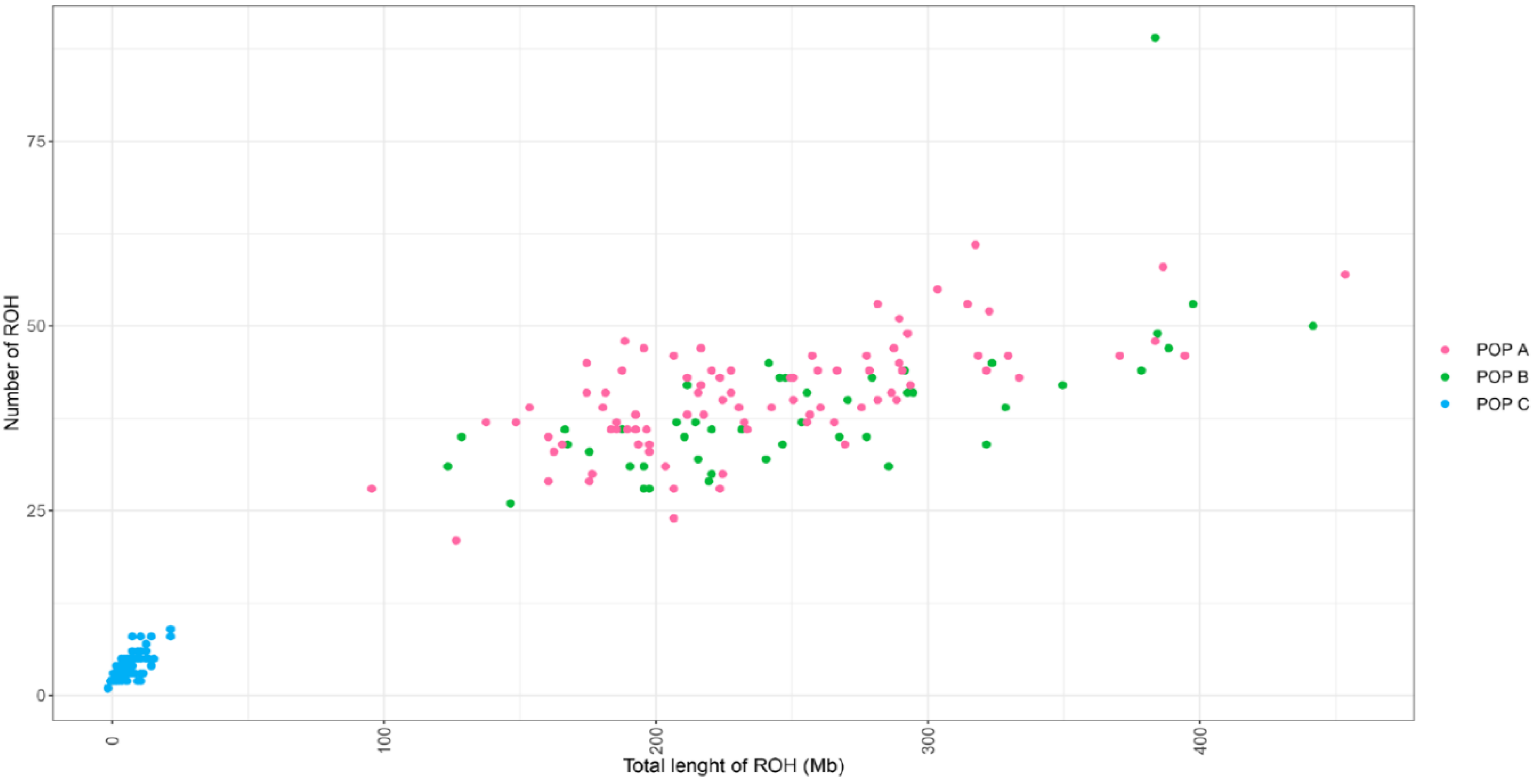
3.2. Distribution of Runs of Homozygosity

We identified ROH in all animals for coho salmon POP A and B, and in 103 out of 104 individuals for POP C. A total of 3250, 1497, and 266 ROH and an average number of 36.93 ± 7.13, 35.65 ± 8.64, 2.65 ± 1.27 ROH per animal were identified for POP A, B and C, respectively. The mean ROH length was 6.47 ± 7.39, 7.17 ± 7.69 and 2.58 ± 2.07 Mb for POP A, B and C, respectively (Table 1) and the longest segment identified was 61.82 Mb, found in chromosome 2 for POP B (Supplementary File 3). The ROH analysis for different length classes suggests that for the three coho salmon populations the genome is mostly composed of a high number of short segments (ROH1–2 Mb, ROH2–4 Mb). No segment was found for ROH>16Mb in POP C.
The average number of ROH identified differs between chromosomes and in low magnitude between populations. For POP A and POP B, most of the chromosomes resulted in the average number of ROH between one and two ROH per animal and more than two ROHs in chromosome Okis6 for POP A and Okis5, Okis18 and Okis19 for POP B, whereas for POP C all chromosomes have less than one ROH per individual (Figure 2). The average ROH length also differs between chromosomes and the population. POP A has two chromosomes (Okis5 and Okis11) with ROH segments greater than 10 Mb. POP B has five chromosomes (Okis3, Okis4, Okis6, Okis11 and Okis14) with ROH segments greater than 10 Mb; while all chromosomes in POP C have ROH segments smaller than 7 Mb (Figure 3).
Figure 4 shows the relationship between the total number of ROH and the total length of ROH for each animal across the three populations. A considerable difference between POP C and POP A or B was found. For POP C, all animals have a small number of ROH (<8) with total length <25 Mb, whereas most individuals in POP A and B have at least 20 ROHs with a total length >100 Mb, with some individuals with segments covering more than 300 Mb. The number of ROHs and segment length per animal and per chromosome are shown in Supplementary File 3. The high number of segments >10 Mb in Okis5, Okis6 and Okis28, especially for POP A and B, suggests recent events of inbreeding, whereas the small segments as in Okis20 for POP A and B, and for most of the chromosomes for POP C, suggests more ancient inbreeding.

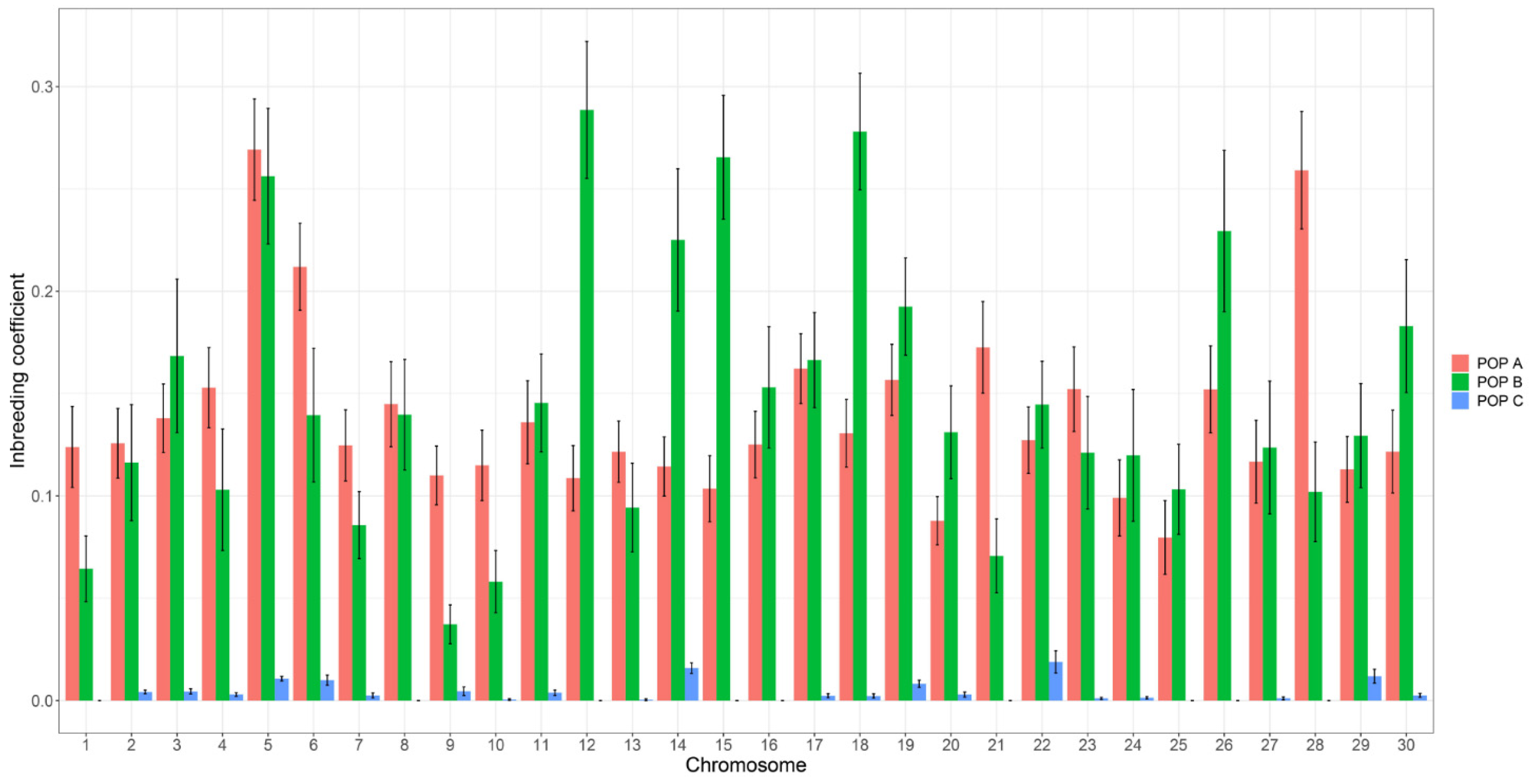
3.3. Genomic- and Pedigree-Based Inbreeding

We used four different methods to estimate the inbreeding coefficient, from the information of 102 K markers and pedigree data (Table 2). The average inbreeding coefficient estimated using ROH was different between ROH classes, the values decreased when the ROH length segments increased for all populations. The mean value for FROHALL was the same for both POP A and B (0.142 and 0.152, respectively), but it was significantly different (p < 0.05) for POP C (0.004) when compared to POP A or B. The FHOM resulted in the lowest inbreeding values ranging from −0.036 to −0.105 for POP A and C, respectively. The mean value for FGRM was different (p < 0.05) between the three populations, the highest and lowest values were reported for POP B and C, respectively, whereas the FPED value was not different between POP A and B, but was significantly lower for POP C (0.002, p < 0.05). Additionally, we estimated the inbreeding coefficient based on the ROH per chromosome (Figure 5). POP A and B had the most chromosomes with inbreeding values higher than 0.2, as in Okis5, Okis6 and Okis28 for POP A, and Okis5, Okis12, Okis14, Okis18 and Okis26 for POP B, whereas lower values were found for POP C and for most of the chromosomes the inbreeding was equal to zero.
The Pearson correlation between different genomic methods to estimate the inbreeding coefficient suggested a high positive correlation (>0.82, p < 0.001) for POP A and POP B (Supplementary File 4 and 5, respectively). Correlation between different ROH length classes decreased in function with the comparison between shorter and longer segments, e.g., highest correlation between ROH1–2 Mb and ROH2–4 Mb and lowest between ROH1–2 Mb and ROH>16Mb. The lowest correlation values among genomic methods was reported between ROH>16Mb and both ROHHOM and ROHGRM. In addition, for POP A and POP B low correlation values were found, respectively, ranging from 0.35 to 0.39 (p < 0.01), between genomic methods and FPED.
Different patterns of correlations were observed for POP C, compared to POP A and B, probably due to the low inbreeding level of this recently admixed population. Medium to high positive correlation was reported between the ROH classes (0.54 to 0.94, p < 0.001), and a correlation equal to unity was observed between ROHHOM and ROHGRM. For other correlations, small values (ranged from 0.28 to 0.34) or not different from zero were observed (Supplementary File 6).
The across-populations Pearson correlation coefficients between different genomic- and pedigree-based inbreeding estimates ranged between 0.56 and 1.00, with the minimum and maximum correlation values found between FHOM—FPED and FROH1–2 MB—FROH2–4 MB—FROH4–8 MB comparisons, respectively. All correlation values among inbreeding coefficient calculated for all individuals across populations are shown in Supplementary File 7.

4. Discussion

The first two principal components explained more than 29% of the total genetic variation for the three populations studied, which were separated into three different clusters. The admixture results are in agreement with the recent event of hybridization of POP A and B to generate POP C, where the genetic differentiation between POP A and B may have been be partly generated by differences in the base population, which can have a pronounced effect on allele frequencies [47]. In addition, considering that POP A and B have been independently selected by at least eight generations each, differences in the selection processes, as well as the environmental conditions and drift, may have influenced the differences observed in Supplementary File 2.
The ROH patterns seem to be differentially distributed within specific genomic regions, same as the inbreeding values between chromosomes. The highest autozygosity, e.g., in chromosome Okis5 and Okis6 for POP A and B, is likely the consequence of artificial selection [28], considering that these populations have been under genetic selection for harvest weight for at least eight generations. A ROH study in humans [48] suggested that the homozygosity segments are more common in regions with high linkage disequilibrium (LD) and low recombination rates. Thus the highest mean levels of LD found in Okis5 and Okis6 in animals from the same populations [39] are in accordance with the two chromosomes with the larger ROH sizein the present study.
Differences in the number of ROH and segment length was observed within and across populations. The greater number of ROH in POP A compared to POP B can be due to higher sample size in the former, considering that the average number of ROH per animal had small variation between populations. The differences in average ROH length may be due to recent inbred mating or other demographic processes along the time in the different populations, which can generate different distribution of long and short ROH segments [49]. Furthermore, the intense artificial selection might have altered the allele frequency and increase the IBD haplotypes and created long ROH in specific regions of the genome [28]. In contrast, the shorter segments and smaller number of ROH in POP C when compared against both POP A and B may be the result of recent population admixture between these populations. Furthermore, animals from the same population might have the same total ROH lengths but a variable number of segments, which is probably the result of different distances from common ancestors [25]. Interestingly, for both POP A and B, the length class ROH2–4 Mb has more ROH than ROH1–2 Mb. These differences can be due to the criteria adopted to identify ROH or an inherent characteristic of these populations. There is no consensus on the best parameters to characterize ROH patterns [36]; thus, here we used the minimum number of 50 SNPs and the length of 1 Mb to define a ROH segment. We chose the current parameters due to the historical demographics of coho salmon in Chile. The ROH2–4 Mb should date from about 20 generations ago (approximately 40 years considering the generation interval of two years), which corresponds to the introduction of coho salmon in Chile at the end of the 1970s, to begin the establishment of Chilean brood stocks [2,39].
Based on information of ROH length it is possible to infer the number of generations for inbreeding events [50]. The ROH due to ancient origin tend to be shorter, e.g., ROH1–2 Mb, ROH2–4 Mb and ROH4–8 Mb date from 50, 20 and 12.5 generations ago, respectively. In contrast, recent ROH are longer, due to the small probability of breaking down the segments that are IBD by means of recombination events. Thus, the ROH8–16 Mb and ROH>16 Mb are dated to six and three generations ago, respectively [22,50]. For both POP A and B it was possible to identify short and long segments in most of the animals analyzed, whereas in the POP C a small number of animals (n = 7) presented ROH8–16 Mb and none ROH>16 Mb.
In recent years, some studies have investigated different genomic methods to estimate inbreeding coefficients in livestock [11,25,28,35,51,52], pigs [29,30,53,54] and goats [55,56,57]. Recently, ROH studies in rainbow trout [36] and turbot [58] reported different average ROH length for these aquaculture species; 4 Mb and 0.77 Mb rainbow trout and turbot, respectively. These differences can be explained due to the genome size, that is 3.5-fold smaller in turbot [58], and also based in different demographic history in the populations assessed. The greater average ROH segments found in the present study (6.6 Mb and 7.2 Mb for POP A and POP B, respectively) are most likely due to high selection intensity during almost eight generations in these coho salmon population and the mate allocation strategies that resulted in high level of inbreeding, and consequently longer ROH segments. However, this is the first study aimed at characterizing the ROH patterns and comparing different genomic- and pedigree-based methods to estimate inbreeding coefficients in farmed coho salmon populations. The pedigree-based inbreeding coefficient, is a simple method that requires recording genealogy information, but does not account for the autozygosity differences among animals with the same inbreeding history. Furthermore, considering that the founder animals are unrelated pedigree-based inbreeding estimates may lead to underestimation of autozygosity levels [11]. In contrast, with the availability of high-density SNP information, inbreeding can be accurately measured, even without pedigree information [15]. ROH can provide a better estimation of whole-genome autozygosity levels, by identifying IBD segments with great accuracy [51], and based on length of the ROH segments the ancient and contemporary inbreeding can be reported [29].
A comparison of inbreeding coefficients, showed that FGRM gave the highest values, especially for B and C, probably because the alleles IBD and IBS are not differentiated for FGRM [11]. This result is in agreement with results previously found in humans, cattle, and simulation studies [11,15,16]. FHOM resulted in negative inbreeding values for all populations, suggesting that the individuals have lower levels of homozygosity than expected in the reference population under Hardy-Weinberg equilibrium [59] and underestimated values should be expected [60]. The FPED for POP A and POP B were smaller than values estimated using FROHALL and FGRM, but are in accordance with the values estimated for the same populations using previous generations [8,10]. The FPED can be easily underestimated when pedigree information of less than 20 generations is used [60]. The difference between FROH and FPED could also be due to the unknown pedigree information before base population, which in practical terms means that inbreeding levels for founding animals were not zero.
ROH can be identified for each genotyped animal, allowing to detect specific location in the genome with high levels of autozygosity, i.e., along chromosomes [61]. In this regard, we used the Pearson correlation to evaluate the agreement between FROH and other approaches to estimate genomic inbreeding (FGRM and FHOM). Correlations between FGRM and FROH decreased while decreasing size of ROH classes probably due to that G matrix that is based in individual loci, whereas FROH is based on chromosomal segments, and the FGRM cannot distinguish between alleles that are IBD and IBS [62]. Another reason which may explain this pattern is that ROH is the sum of large and short segments, and ROH classes of smaller size could be more informative on the homozygosity status across the genome when compared to classes of larger ROH segments. It has also been previously suggested that both FGRM and FHOM are strongly dependent on allele frequencies, especially for populations with divergent allele frequencies (high level of heterozygosity and some rare alleles with small frequency), which can result in misleading IBD [51,63]. The high correlations (>0.80) found between FROH and other genomic inbreeding estimates for POP A and B, and moderate to strong positive correlation between genomics methods used to estimate inbreeding coefficients has been reported for different species [27,29,62,64], suggesting that the extent of homozygosity in a genome can be accurately used to predict the proportion of the genome that is IBD. In contrast, we found low correlation between FROH in different length classes and FGRM and FHOM for the POP C, which makes sense considering that this is a recently admixed population, and the correlation might be affected by the average degree of actual homozygosity of population [27,35].
The genomic-based inbreeding method correlated moderately or poorly with pedigree data, showing values lower than 0.39. Similarly weak or no correlation was reported for cattle [24,51,52], whereas a moderate to strong positive correlation was described by some authors [15,16,35,65]. An increase in the correlation between genomic- and pedigree-based inbreeding as the pedigree depth increases is expected [24]. Here we used the complete pedigree information of nine generations for both POP A and POP B, whereas for POC C, a pedigree depth of eight generations was used. In a previous pedigree-based inbreeding study using the same broodstock population of POP A (7th generation) and POP B (8 th generation), an increasing tendency for inbreeding values in the last four generations was reported for both populations [8] and a continued inbreeding accumulation until 9 th generation used in our study is well-known. Thus, we expected a higher correlation between long ROH segments (ROH8–16 Mb, and ROH>16 Mb) and FPED values. The weak or no correlation may be explained by the depth of pedigree records [61], incorrect or incomplete pedigree information [51]. The FPED assumed that the founder individuals are unrelated [11], does not consider the stochastic nature of recombination and the persistence of ancestral short segments through time, due to the lack of recombination in specific regions [27]. These facts suggest that the FPED may not reflect true inbreeding values. In addition, the correlation between genomic and pedigree-based inbreeding can be also affected by the parameters to determine ROH [35,36,66] and the population sample size [15,24]. Here we chose the parameters to identify ROH segments based on those reported in previous studies [27,36,52,65,67,68]. Regarding sample size, the POP B is the population with the smallest sample size (n = 45); however, was the only one that resulted in significant correlations between genomic- and pedigree-based inbreeding levels. Moreover, various studies on the characterization of ROH patterns in production species used similar or smaller sample size [26,35,36,69].
A relatively large effective population size (Ne), ranged from 50 to 200, is recommended to maintain the control of inbreeding in the medium-term [70]. However, decline in the historical Ne was reported for animals from the same population as POP A [39]. The reduction may be due to the prioritization of genetic gain using high selection pressure without putting strong control on the family contribution for each generation [8]. Consequently, mating close relatives is more probable, which results in a high level of inbreeding and the creation of long ROH segments for both POP A and B. Therefore, to increase the effective population size and to limit the inbreeding level [8], POP C was generated. According to our results, this strategy was effective in reducing the inbreeding levels and changing the patterns of ROH, clearly differentiating from POP A and B. These results are in accordance with some studies [15,35,55,57] that suggest that high heterogeneity populations due admixture or crossbreeding lines contributed to the breakdown of long homozygous segments and reduced the inbreeding levels in captive populations.

5. Conclusions

We found different numbers and lengths of runs of homozygosity in three coho salmon populations included in the study. Moreover, the inbreeding coefficient estimated using genomic or pedigree-based methods varied among populations. The higher correlations between genomic-based inbreeding methods, except for POP C and most likely due to recent admixture history, suggests that genomic approaches are more accurate to estimate autozygosity levels, and thus, must be used as the methods of choice when pedigree information is inaccurate, incomplete or unavailable.

Supplementary Materials

The following are available online at https://www.mdpi.com/2073-4425/11/5/490/s1, Table S1: Summary of results from quality control of SNP genotypes. Figure S1: Admixture clustering of the three coho salmon population for K = 4. Figure S2: Runs of homozygosity patterns for all chromosome coho salmon populations. Figure S3: Scatterplots and Pearson correlation of inbreeding coefficients for POP A. Figure S4: Scatterplots and Pearson correlation of inbreeding coefficients for POP B. Figure S5: Scatterplots and Pearson correlation of inbreeding coefficients for POP C. Figure S6: Scatterplots and Pearson correlation of inbreeding coefficients across coho salmon populations.

Author Contributions

G.M.Y. performed the analysis and wrote the initial version of the manuscript. P.C. and R.M.-N. contribute with writing. B.F.K. develop the SNP array. J.M.Y. conceived and designed the study; contributed to the discussion and writing. All authors have read and agreed to the published version of the manuscript.

Funding

This research was partially funded by Government of Canada through EPIC4 (Enhanced Production in Coho: Culture, Community, Catch) from Genome Canada, Genome British Columbia, and Genome Quebec.

Acknowledgments

We thank the Government of Canada through Genome Canada, Genome British Columbia, and Genome Quebec to supported this research that was carried out in conjunction with the projected EPIC4 (Enhanced Production in Coho: Culture, Community, Catch). We also would like to acknowledge Pesquera Antares S.A., which provided the fish used in this study. GMY is supported by Fondecyt/Conicyt Postdoctoral Grant n. 3190553, and JMY is supported by Núcleo Milenio INVASAL funded by Chile’s government program, Iniciativa Cientifica Milenio from Ministerio de Economia, Fomento y Turismo.

Conflicts of Interest

The authors declare that the research was conducted in the absence of any commercial or financial relationships that could be construed as a potential conflict of interest.

References

  1. Groot, C.; Margolis, L. Pacific Salmon Life Histories; UBC Press: Vancouver, BC, Canada, 1991; ISBN 9780774803595. [Google Scholar]
  2. Neira, R.; Lhorente, J.P.; Yáñez, J.M.; Araneda, M.; Filp, M. Evolution of Coho Salmon (Oncorhynchus kisutch) Breeding Programs. In Proceedings of the 10th World Congress of Genetics Applied to Livestock Production, Vancouver, BC, Canada, 17–22 August 2014; pp. 1–6. [Google Scholar]
  3. Lhorente, J.P.; Araneda, M.; Neira, R.; Yáñez, J.M. Advances in genetic improvement for salmon and trout aquaculture: The Chilean situation and prospects. Rev. Aquac. 2019, 11, 340–353. [Google Scholar] [CrossRef]
  4. Gjedrem, T. Genetic improvement of cold-water fish species. Aquac. Res. 2000, 31, 25–33. [Google Scholar] [CrossRef]
  5. Gjedrem, T.; Robinson, N.; Rye, M. The importance of selective breeding in aquaculture to meet future demands for animal protein: A review. Aquaculture 2012, 350–353, 117–129. [Google Scholar] [CrossRef]
  6. Howard, J.T.; Pryce, J.E.; Baes, C.; Maltecca, C. Invited review: Inbreeding in the genomics era: Inbreeding, inbreeding depression, and management of genomic variability. J. Dairy Sci. 2017, 100, 6009–6024. [Google Scholar] [CrossRef] [PubMed]
  7. Gallardo, A.; Garcı, X.; Paul, J.; Neira, R. Inbreeding and inbreeding depression of female reproductive traits in two populations of Coho salmon selected using BLUP predictors of breeding values. Aquaculture 2004, 234, 111–122. [Google Scholar] [CrossRef]
  8. Yáñez, J.M.; Bassini, L.N.; Filp, M.; Lhorente, J.P.; Ponzoni, R.W.; Neira, R. Inbreeding and effective population size in a coho salmon (Oncorhynchus kisutch) breeding nucleus in Chile. Aquaculture 2014, 420–421, S15–S19. [Google Scholar] [CrossRef]
  9. Ponzoni, R.W.; Khaw, H.L.; Nguyen, N.H.; Hamzah, A. Inbreeding and effective population size in the Malaysian nucleus of the GIFT strain of Nile tilapia (Oreochromis niloticus). Aquaculture 2010, 302, 42–48. [Google Scholar] [CrossRef]
  10. Yoshida, G.M.; Yáñez, J.M.; de Oliveira, C.A.L.; Ribeiro, R.P.; Lhorente, J.P.; de Queiroz, S.A.; Carvalheiro, R. Mate selection in aquaculture breeding using differential evolution algorithm. Aquac. Res. 2017, 48, 5490–5497. [Google Scholar] [CrossRef]
  11. Forutan, M.; Ansari Mahyari, S.; Baes, C.; Melzer, N.; Schenkel, F.S.; Sargolzaei, M. Inbreeding and runs of homozygosity before and after genomic selection in North American Holstein cattle. BMC Genom. 2018, 19, 98. [Google Scholar] [CrossRef]
  12. Cassell, B.G.; Adamec, V.; Pearson, R.E. Effect of Incomplete Pedigrees on Estimates of Inbreeding and Inbreeding Depression for Days to First Service and Summit Milk Yield in Holsteins and Jerseys. J. Dairy Sci. 2003, 86, 2967–2976. [Google Scholar] [CrossRef]
  13. Curik, I.; Ferenčaković, M.; Sölkner, J. Inbreeding and runs of homozygosity: A possible solution to an old problem. Livest. Sci. 2014, 166, 26–34. [Google Scholar] [CrossRef]
  14. VanRaden, P.M. Efficient Methods to Compute Genomic Predictions. J. Dairy Sci. 2008, 91, 4414–4423. [Google Scholar] [CrossRef] [PubMed] [Green Version]
  15. Marras, G.; Gaspa, G.; Sorbolini, S.; Dimauro, C.; Ajmone-Marsan, P.; Valentini, A.; Williams, J.L.; Macciotta, N.P.P. Analysis of runs of homozygosity and their relationship with inbreeding in five cattle breeds farmed in Italy. Anim. Genet. 2015, 46, 110–121. [Google Scholar] [CrossRef] [PubMed]
  16. McQuillan, R.; Leutenegger, A.-L.; Abdel-Rahman, R.; Franklin, C.S.; Pericic, M.; Barac-Lauc, L.; Smolej-Narancic, N.; Janicijevic, B.; Polasek, O.; Tenesa, A.; et al. Runs of Homozygosity in European Populations. Am. J. Hum. Genet. 2008, 83, 359–372. [Google Scholar] [CrossRef] [Green Version]
  17. Brüniche-Olsen, A.; Kellner, K.F.; Anderson, C.J.; DeWoody, J.A. Runs of homozygosity have utility in mammalian conservation and evolutionary studies. Conserv. Genet. 2018, 19, 1295–1307. [Google Scholar] [CrossRef]
  18. Falconer, D.S.; Mackay, T.F.C. Introduction to Quantitative Genetics; Pearson, P.H., Ed.; Longman: Harlow, UK, 1996. [Google Scholar]
  19. Peripolli, E.; Munari, D.P.; Silva, M.V.G.B.; Lima, A.L.F.; Irgang, R.; Baldi, F. Runs of homozygosity: Current knowledge and applications in livestock. Anim. Genet. 2017, 48, 255–271. [Google Scholar] [CrossRef]
  20. MacLeod, I.M.; Larkin, D.M.; Lewin, H.A.; Hayes, B.J.; Goddard, M.E. Inferring demography from runs of homozygosity in whole-genome sequence, with correction for sequence errors. Mol. Biol. Evol. 2013, 30, 2209–2223. [Google Scholar] [CrossRef] [Green Version]
  21. Sams, A.J.; Boyko, A.R. Fine-Scale Resolution of Runs of Homozygosity Reveal Patterns of Inbreeding and Substantial Overlap with Recessive Disease Genotypes in Domestic Dogs. G3 2019, 9, 117–123. [Google Scholar] [CrossRef] [Green Version]
  22. Kirin, M.; McQuillan, R.; Franklin, C.S.; Campbell, H.; McKeigue, P.M.; Wilson, J.F. Genomic Runs of Homozygosity Record Population History and Consanguinity. PLoS ONE 2010, 5, e13996. [Google Scholar] [CrossRef] [Green Version]
  23. Nothnagel, M.; Lu, T.T.; Kayser, M.; Krawczak, M. Genomic and geographic distribution of SNP-defined runs of homozygosity in Europeans. Hum. Mol. Genet. 2010, 19, 2927–2935. [Google Scholar] [CrossRef] [Green Version]
  24. Gurgul, A.; Szmatoła, T.; Topolski, P.; Jasielczuk, I.; Żukowski, K.; Bugno-Poniewierska, M. The use of runs of homozygosity for estimation of recent inbreeding in Holstein cattle. J. Appl. Genet. 2016, 57, 527–530. [Google Scholar] [CrossRef] [PubMed]
  25. Mészáros, G.; Boison, S.A.; Pérez O’Brien, A.M.; Ferenčaković, M.; Curik, I.; Da Silva, M.V.B.; Utsunomiya, Y.T.; Garcia, J.F.; Sölkner, J. Genomic analysis for managing small and endangered populations: A case study in Tyrol Grey cattle. Front. Genet. 2015, 6, 173. [Google Scholar] [PubMed] [Green Version]
  26. Signer-Hasler, H.; Burren, A.; Neuditschko, M.; Frischknecht, M.; Garrick, D.; Stricker, C.; Gredler, B.; Bapst, B.; Flury, C. Population structure and genomic inbreeding in nine Swiss dairy cattle populations. Genet. Sel. Evol. 2017, 49, 83. [Google Scholar] [CrossRef] [PubMed] [Green Version]
  27. Ferenčaković, M.; Hamzić, E.; Gredler, B.; Solberg, T.R.; Klemetsdal, G.; Curik, I.; Sölkner, J. Estimates of autozygosity derived from runs of homozygosity: Empirical evidence from selected cattle populations. J. Anim. Breed. Genet. 2013, 130, 286–293. [Google Scholar] [CrossRef] [PubMed]
  28. Kim, E.-S.; Cole, J.B.; Huson, H.; Wiggans, G.R.; Van Tassell, C.P.; Crooker, B.A.; Liu, G.; Da, Y.; Sonstegard, T.S. Effect of Artificial Selection on Runs of Homozygosity in U.S. Holstein Cattle. PLoS ONE 2013, 8, e80813. [Google Scholar] [CrossRef] [Green Version]
  29. Gomez-Raya, L.; Rodríguez, C.; Barragán, C.; Silió, L. Genomic inbreeding coefficients based on the distribution of the length of runs of homozygosity in a closed line of Iberian pigs. Genet. Sel. Evol. 2015, 47, 81. [Google Scholar] [CrossRef] [Green Version]
  30. Xu, Z.; Sun, H.; Zhang, Z.; Zhao, Q.; Olasege, B.S.; Li, Q.; Yue, Y.; Ma, P.; Zhang, X.; Wang, Q.; et al. Assessment of Autozygosity Derived From Runs of Homozygosity in Jinhua Pigs Disclosed by Sequencing Data. Front. Genet. 2019, 10, 274. [Google Scholar] [CrossRef]
  31. Ai, H.; Huang, L.; Ren, J. Genetic Diversity, Linkage Disequilibrium and Selection Signatures in Chinese and Western Pigs Revealed by Genome-Wide SNP Markers. PLoS ONE 2013, 8, e56001. [Google Scholar] [CrossRef] [Green Version]
  32. Beynon, S.E.; Slavov, G.T.; Farré, M.; Sunduimijid, B.; Waddams, K.; Davies, B.; Haresign, W.; Kijas, J.; MacLeod, I.M.; Newbold, C.J.; et al. Population structure and history of the Welsh sheep breeds determined by whole genome genotyping. BMC Genet. 2015, 16, 65. [Google Scholar] [CrossRef] [Green Version]
  33. Manunza, A.; Noce, A.; Serradilla, J.M.; Goyache, F.; Martínez, A.; Capote, J.; Delgado, J.V.; Jordana, J.; Muñoz, E.; Molina, A.; et al. A genome-wide perspective about the diversity and demographic history of seven Spanish goat breeds. Genet. Sel. Evol. 2016, 48, 52. [Google Scholar] [CrossRef] [Green Version]
  34. Ghoreishifar, S.M.; Moradi-Shahrbabak, H.; Fallahi, M.H.; Moradi-Shahrbabak, M.; Abdollahi-Arpanahi, R.; Khansefid, M. Genomic measures of inbreeding coefficients and genome-wide scan for runs of homozygosity islands in Iranian river buffalo, Bubalus bubalis. BMC Genet. 2020, 21, 16. [Google Scholar]
  35. Purfield, D.C.; Berry, D.P.; McParland, S.; Bradley, D.G. Runs of homozygosity and population history in cattle. BMC Genet. 2012, 13, 70. [Google Scholar] [CrossRef] [PubMed] [Green Version]
  36. D’Ambrosio, J.; Phocas, F.; Haffray, P.; Bestin, A.; Brard-Fudulea, S.; Poncet, C.; Quillet, E.; Dechamp, N.; Fraslin, C.; Charles, M.; et al. Genome-wide estimates of genetic diversity, inbreeding and effective size of experimental and commercial rainbow trout lines undergoing selective breeding. Genet. Sel. Evol. 2019, 51, 26. [Google Scholar] [CrossRef] [PubMed] [Green Version]
  37. Yañez, J.M.; Bangera, R.; Lhorente, J.P.; Oyarzún, M.; Neira, R. Quantitative genetic variation of resistance against Piscirickettsia salmonis in Atlantic salmon (Salmo salar). Aquaculture 2013, 414, 155–159. [Google Scholar] [CrossRef]
  38. Yáñez, J.M.; Lhorente, J.P.; Bassini, L.N.; Oyarzún, M.; Neira, R.; Newman, S. Genetic co-variation between resistance against both Caligus rogercresseyi and Piscirickettsia salmonis, and body weight in Atlantic salmon (Salmo salar). Aquaculture 2014, 433, 295–298. [Google Scholar] [CrossRef]
  39. Barria, A.; Christensen, K.A.; Yoshida, G.; Jedlicki, A.; Leong, J.S.; Rondeau, E.B.; Lhorente, J.P.; Koop, B.F.; Davidson, W.S.; Yáñez, J.M. Whole genome linkage disequilibrium and effective population size in a coho salmon (Oncorhynchus kisutch) breeding population using a high density SNP array. Front. Genet. 2019, 10, 498. [Google Scholar] [CrossRef] [Green Version]
  40. Purcell, S.; Neale, B.; Todd-Brown, K.; Thomas, L.; Ferreira, M.A.R.; Bender, D.; Maller, J.; Sklar, P.; de Bakker, P.I.W.; Daly, M.J.; et al. PLINK: A tool set for whole-genome association and population-based linkage analyses. Am. J. Hum. Genet. 2007, 81, 559–575. [Google Scholar] [CrossRef] [Green Version]
  41. R Core Team. R: A Language and Environment for Statistical Computing; R Foundation for Statistical Computing: Vienna, Austria, 2015. [Google Scholar]
  42. Pritchard, J.K.; Stephens, M.; Rosenberg, N.A.; Donnelly, P. Association Mapping in Structured Populations. Am. J. Hum. Genet. 2000, 67, 170–181. [Google Scholar] [CrossRef] [Green Version]
  43. Evanno, G.; Regnaut, S.; Goudet, J. Detecting the number of clusters of individuals using the software structure: A simulation study. Mol. Ecol. 2005, 14, 2611–2620. [Google Scholar] [CrossRef] [Green Version]
  44. Biscarini, F.; Cozzi, P.; Gaspa, G.; Marras, G. Detect Runs of Homozygosity and Runs of Heterozygosity in Diploid Genomes. CRAN. Available online: https://cran.r-project.org/web/checks/check_results_detectRUNS.html (accessed on 24 October 2019).
  45. Wright, S. Genetics of populations. Encycl. Br. 1948, 10, 111–112. [Google Scholar]
  46. Legarra, A.; Aguilar, I.; Misztal, I. A relationship matrix including full pedigree and genomic information. J. Dairy Sci. 2009, 92, 4656–4663. [Google Scholar] [CrossRef] [PubMed] [Green Version]
  47. Allendorf, F.W.; Phelps, S.R. Loss of Genetic Variation in a Hatchery Stock of Cutthroat Trout. Trans. Am. Fish. Soc. 1980, 109, 537–543. [Google Scholar] [CrossRef]
  48. Gibson, J.; Morton, N.E.; Collins, A. Extended tracts of homozygosity in outbred human populations. Hum. Mol. Genet. 2006, 15, 789–795. [Google Scholar] [CrossRef] [PubMed] [Green Version]
  49. Ceballos, F.C.; Joshi, P.K.; Clark, D.W.; Ramsay, M.; Wilson, J.F. Runs of homozygosity: Windows into population history and trait architecture. Nat. Rev. Genet. 2018, 19, 220–234. [Google Scholar] [CrossRef] [PubMed]
  50. Broman, K.W.; Weber, J.L. Long Homozygous Chromosomal Segments in Reference Families from the Centre d’Étude du Polymorphisme Humain. Am. J. Hum. Genet. 1999, 65, 1493–1500. [Google Scholar] [CrossRef] [Green Version]
  51. Zhang, Q.; Calus, M.P.; Guldbrandtsen, B.; Lund, M.S.; Sahana, G. Estimation of inbreeding using pedigree, 50k SNP chip genotypes and full sequence data in three cattle breeds. BMC Genet. 2015, 16, 88. [Google Scholar] [CrossRef] [PubMed] [Green Version]
  52. Peripolli, E.; Stafuzza, N.B.; Munari, D.P.; Lima, A.L.F.; Irgang, R.; Machado, M.A.; Panetto, J.C.d.C.; Ventura, R.V.; Baldi, F.; da Silva, M.V.G.B. Assessment of runs of homozygosity islands and estimates of genomic inbreeding in Gyr (Bos indicus) dairy cattle. BMC Genomics 2018, 19, 34. [Google Scholar] [CrossRef]
  53. Zhang, Z.; Zhang, Q.; Xiao, Q.; Sun, H.; Gao, H.; Yang, Y.; Chen, J.; Li, Z.; Xue, M.; Ma, P.; et al. Distribution of runs of homozygosity in Chinese and Western pig breeds evaluated by reduced-representation sequencing data. Anim. Genet. 2018, 49, 579–591. [Google Scholar] [CrossRef]
  54. Howard, J.T.; Tiezzi, F.; Huang, Y.; Gray, K.A.; Maltecca, C. Characterization and management of long runs of homozygosity in parental nucleus lines and their associated crossbred progeny. Genet. Sel. Evol. 2016, 48, 91. [Google Scholar] [CrossRef] [Green Version]
  55. Cardoso, T.F.; Amills, M.; Bertolini, F.; Rothschild, M.; Marras, G.; Boink, G.; Jordana, J.; Capote, J.; Carolan, S.; Hallsson, J.H.; et al. Patterns of homozygosity in insular and continental goat breeds. Genet. Sel. Evol. 2018, 50, 56. [Google Scholar] [CrossRef] [Green Version]
  56. Bertolini, F.; Cardoso, T.F.; Marras, G.; Nicolazzi, E.L.; Rothschild, M.F.; Amills, M. Genome-wide patterns of homozygosity provide clues about the population history and adaptation of goats. Genet. Sel. Evol. 2018, 50, 59. [Google Scholar] [CrossRef] [PubMed] [Green Version]
  57. Onzima, R.B.; Upadhyay, M.R.; Doekes, H.P.; Brito, L.F.; Bosse, M.; Kanis, E.; Groenen, M.A.M.; Crooijmans, R.P.M.A. Genome-Wide Characterization of Selection Signatures and Runs of Homozygosity in Ugandan Goat Breeds. Front. Genet. 2018, 9, 318. [Google Scholar] [CrossRef] [PubMed]
  58. Morales-González, E.; Saura, M.; Fernández, A.; Fernández, J.; Pong-Wong, R.; Cabaleiro, S.; Martínez, P.; Martín-García, A.; Villanueva, B. Evaluating different genomic coancestry matrices for managing genetic variability in turbot. Aquaculture 2020, 520, 734985. [Google Scholar] [CrossRef]
  59. Wang, J. Marker-based estimates of relatedness and inbreeding coefficients: An assessment of current methods. J. Evol. Biol. 2014, 27, 518–530. [Google Scholar] [CrossRef] [PubMed]
  60. Kardos, M.; Luikart, G.; Allendorf, F.W. Measuring individual inbreeding in the age of genomics: Marker-based measures are better than pedigrees. Heredity 2015, 115, 63–72. [Google Scholar] [CrossRef] [PubMed]
  61. Keller, M.C.; Visscher, P.M.; Goddard, M.E. Quantification of inbreeding due to distant ancestors and its detection using dense single nucleotide polymorphism data. Genetics 2011, 189, 237–249. [Google Scholar] [CrossRef] [Green Version]
  62. Mastrangelo, S.; Tolone, M.; Di Gerlando, R.; Fontanesi, L.; Sardina, M.T.; Portolano, B. Genomic inbreeding estimation in small populations: Evaluation of runs of homozygosity in three local dairy cattle breeds. Animal 2016, 10, 746–754. [Google Scholar] [CrossRef] [Green Version]
  63. Purfield, D.C.; McParland, S.; Wall, E.; Berry, D.P. The distribution of runs of homozygosity and selection signatures in six commercial meat sheep breeds. PLoS ONE 2017, 12, e0176780. [Google Scholar] [CrossRef] [Green Version]
  64. Sumreddee, P.; Toghiani, S.; Hay, E.H.; Roberts, A.; Agrrey, S.E.; Rekaya, R. Inbreeding depression in line Hereford cattle population using pedigree and genomic information. J. Anim. Sci. 2019, 97, 1–18. [Google Scholar] [CrossRef]
  65. Zavarez, L.B.; Utsunomiya, Y.T.; Carmo, A.S.; Neves, H.H.R.; Brien, A.M.P.O.; Curik, I.; Cole, J.B.; Carvalheiro, R.; Feren, M.; Tassell, V.; et al. Assessment of autozygosity in Nellore cows (Bos indicus) through high-density SNP genotypes. Front. Genet. 2015, 6, 1–8. [Google Scholar] [CrossRef] [Green Version]
  66. Lencz, T.; Lambert, C.; DeRosse, P.; Burdick, K.E.; Morgan, T.V.; Kane, J.M.; Kucherlapati, R.; Malhotra, A.K. Runs of homozygosity reveal highly penetrant recessive loci in schizophrenia. Proc. Natl. Acad. Sci. USA 2007, 104, 19942–19947. [Google Scholar] [CrossRef] [PubMed] [Green Version]
  67. Bosse, M.; Megens, H.-J.; Madsen, O.; Paudel, Y.; Frantz, L.A.F.; Schook, L.B.; Crooijmans, R.P.M.A.; Groenen, M.A.M. Regions of Homozygosity in the Porcine Genome: Consequence of Demography and the Recombination Landscape. PLoS Genet. 2012, 8, e1003100. [Google Scholar] [CrossRef] [PubMed] [Green Version]
  68. Traspov, A.; Deng, W.; Kostyunina, O.; Ji, J.; Shatokhin, K.; Lugovoy, S.; Zinovieva, N.; Yang, B.; Huang, L. Population structure and genome characterization of local pig breeds in Russia, Belorussia, Kazakhstan and Ukraine. Genet. Sel. Evol. 2016, 48, 16. [Google Scholar] [CrossRef] [PubMed] [Green Version]
  69. Goszczynski, D.; Molina, A.; Terán, E.; Morales-Durand, H.; Ross, P.; Cheng, H.; Giovambattista, G.; Demyda-Peyrás, S. Runs of homozygosity in a selected cattle population with extremely inbred bulls: Descriptive and functional analyses revealed highly variable patterns. PLoS ONE 2018, 13, e0200069. [Google Scholar] [CrossRef] [PubMed] [Green Version]
  70. Smitherman, R.O.; Tave, D. Maintenance of genetic quality in cultured tilapia. Asian Fish. Sci. 1987, 1, 75–82. [Google Scholar]
Figure 1. Principal component analysis of the autosomal genotypic data of three coho salmon populations.
Genes 11 00490 g001
Figure 2. Distribution of the average number of ROH per individual for each chromosome in three coho salmon populations.
Genes 11 00490 g002
Figure 3. Average ROH length and standard error bars for each chromosome in three coho salmon populations.
Genes 11 00490 g003
Figure 4. Relationship between the number of runs of homozygosity (ROH) and total length of ROH (Mb) per individual from each population.
Genes 11 00490 g004
Figure 5. Distribution of average inbreeding coefficients estimated using ROH for each chromosome in three coho salmon populations. Standard error bars were computed among individuals from the same population.
Genes 11 00490 g005
Table 1. Total number of runs of homozygosity (ROH) (N) per class, the average number of ROH per individual (N Mean) and average length (Mb) considered all ROH and by classes for three coho salmon populations.
ClassPOP A POP B POP C
NN MeanLengthNN MeanLengthNN MeanLength
ROHALL32507.39 (3.75)6.47 (7.39) 14976.65 (3.84)7.17 (7.69) 2660.54 (0.85)2.58 (2.07)
ROH1–2 Mb8479.63 (3.16)1.46 (0.29) 3417.58 (3.60)1.46 (0.29) 1581.60 (1.06)1.40 (0.26)
ROH2–4 Mb93710.65 (3.28)2.89 (0.58) 4008.89 (4.33)2.84 (0.53) 580.59 (0.69)2.86 (0.58)
ROH4–8 Mb6807.73 (2.73)5.59 (1.07) 3106.89 (3.74)5.56 (1.03) 430.43 (0.59)5.11 (1.14)
ROH8–16 Mb4635.26 (2.26)11.31 (2.32) 2605.78 (3.06)11.45 (2.25) 70.07 (0.26)11.54 (0.04)
ROH>16 Mb3233.67 (1.75)24.93 (7.68) 1864.13 (2.58)23.69 (8.08) 00-
Standard deviation in brackets.
Table 2. The number of individuals (N), mean and standard deviation (SD) of inbreeding coefficients using runs of homozygosity (FROH) for different ROH length, based on the excess of homozygosity (FHOM), genomic relationship matrix (FGRM) and pedigree-based relationship matrix (FPED) for each coho salmon population.
ClassPOP A POP B POP C
NMeanSDNMeanSDNMeanSD
FROH1–2 Mb880.142 a0.038 450.152 a0.044 1030.004 b0.003
FROH2–4 Mb880.133 a0.038 450.145 a0.044 730.003 b0.003
FROH4–8 Mb880.115 a0.037 450.129 a0.043 470.002 b0.002
FROH8–16 Mb880.090 a0.036 450.104 a0.043 70.000 b0.002
FROH>16 Mb850.054 a0.028 450.062 a0.036 ---
FROHALL880.142 a0.038 450.152 a0.044 1030.004 b0.003
FHOM88−0.036 b0.048 45−0.069 a0.056 104−0.105 c0.011
FGRM880.145 b0.037 450.193 a0.040 1040.051 c0.009
FPED880.071 a0.021 450.076 a0.027 1040.002 b0.012
Different letters in each row indicate statistical significance for the comparison of methods for inbreeding estimation within populations (p < 0.05).

