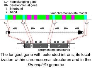
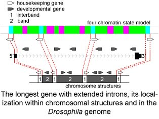
Genes Containing Long Introns Occupy Series of Bands and Interbands in Drosophila melanogaster Polytene Chromosomes

 , ,
, ,
Abstract
1. Introduction
2. Materials and Methods
2.1. Fly Stock
2.2. Fluorescence In Situ Hybridization
2.3. Bioinformatic Methods
3. Results
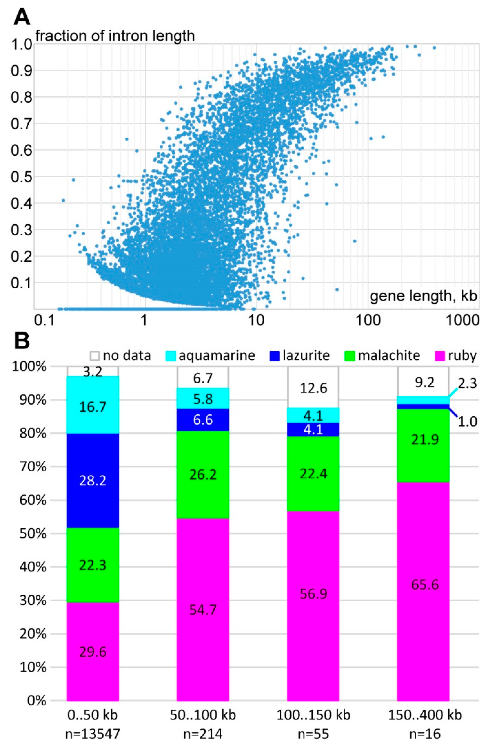
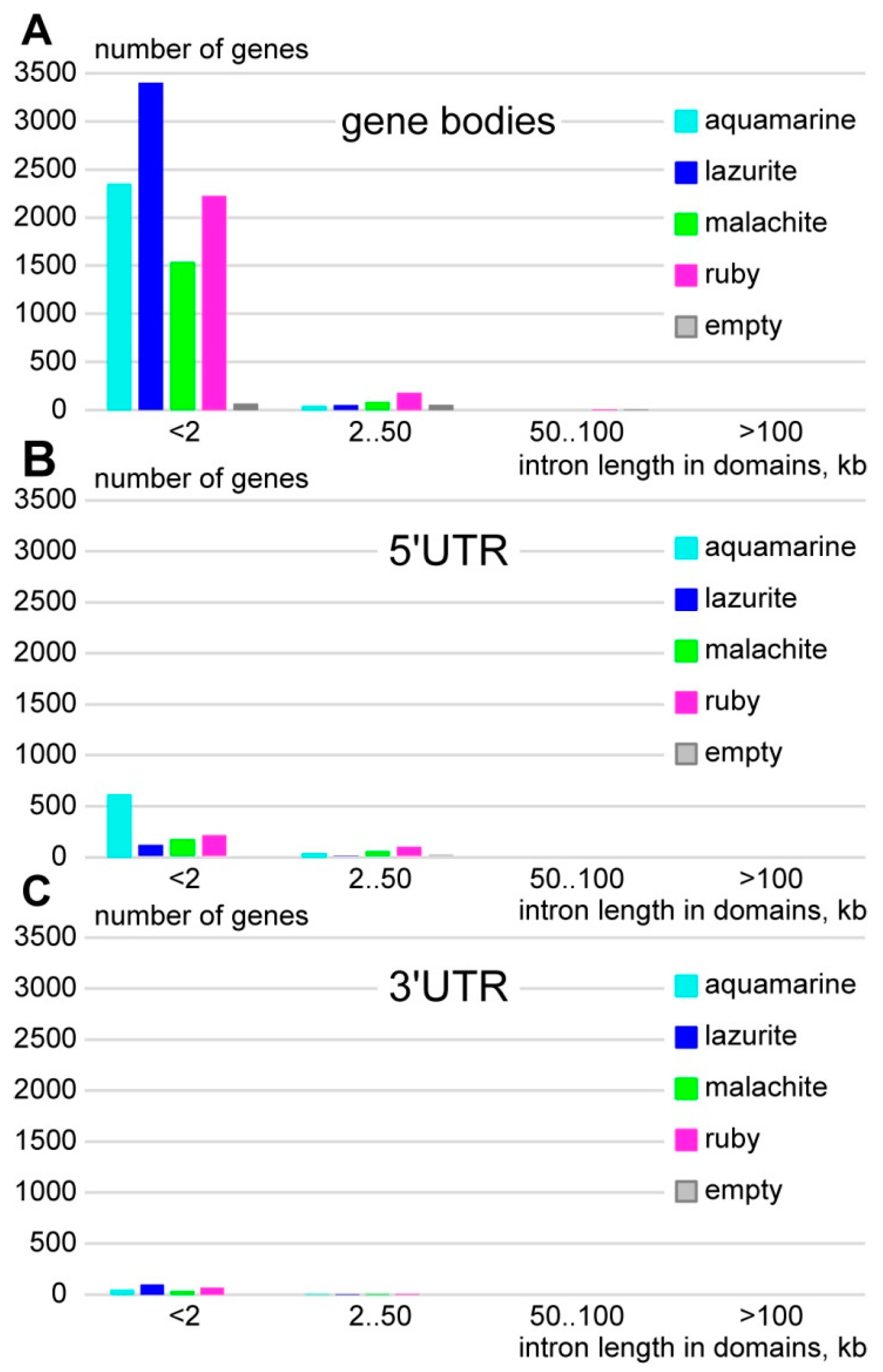
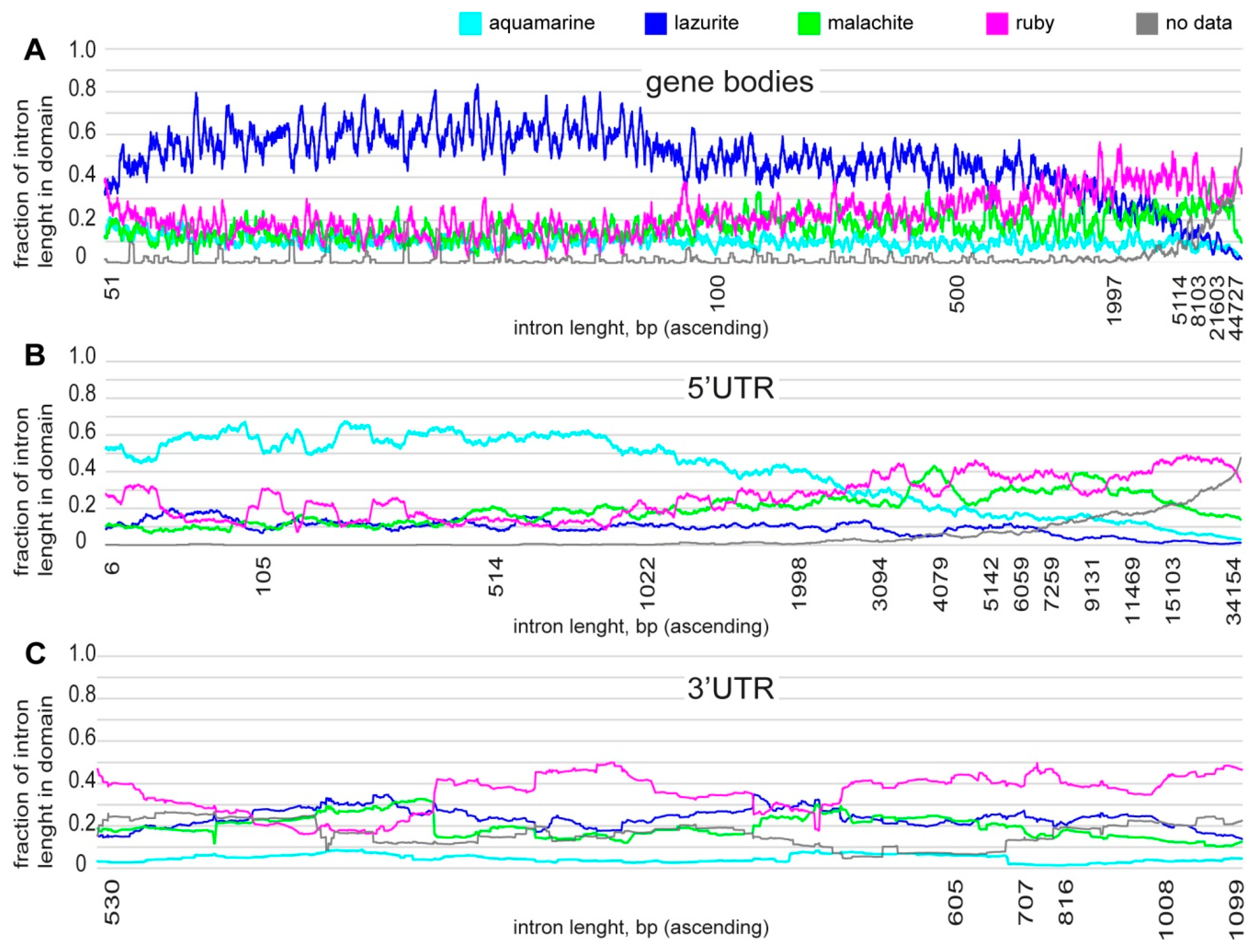
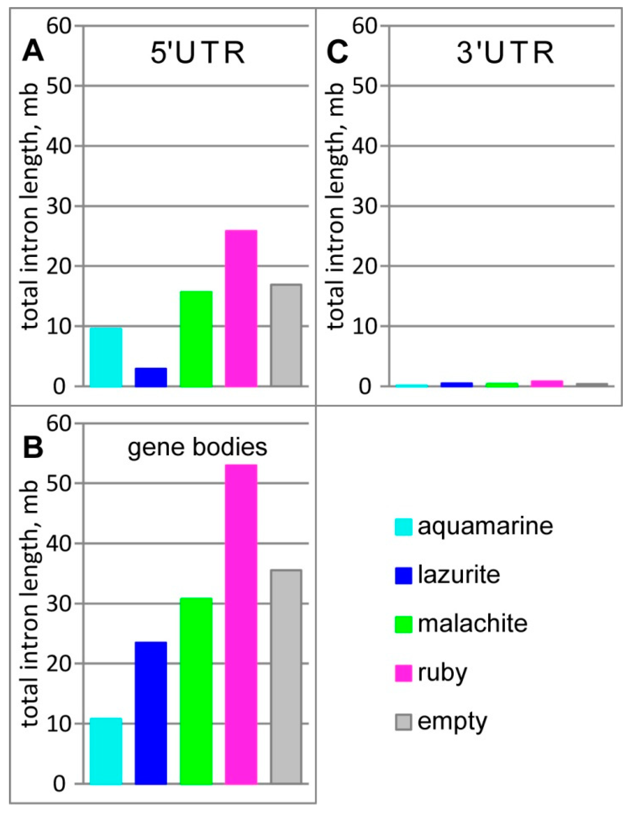
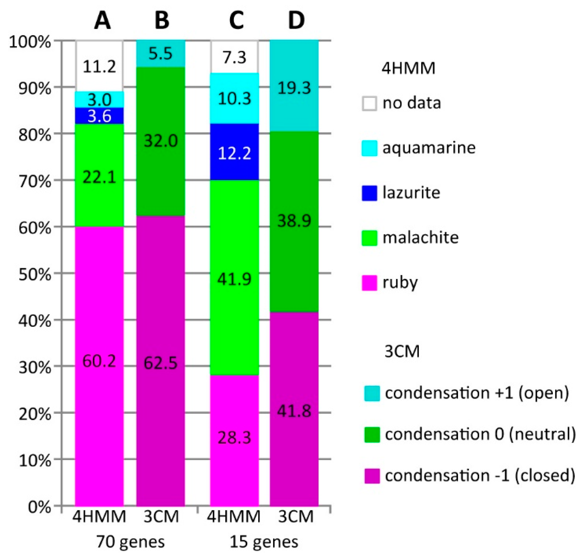
3.1. Characteristics of Introns and Genes Located In Different Chromatin Domains In The Drosophila Genome
3.2. Long Genes Mapping In Polytene Chromosomes Bands and Interbands
3.2.1. CG3777
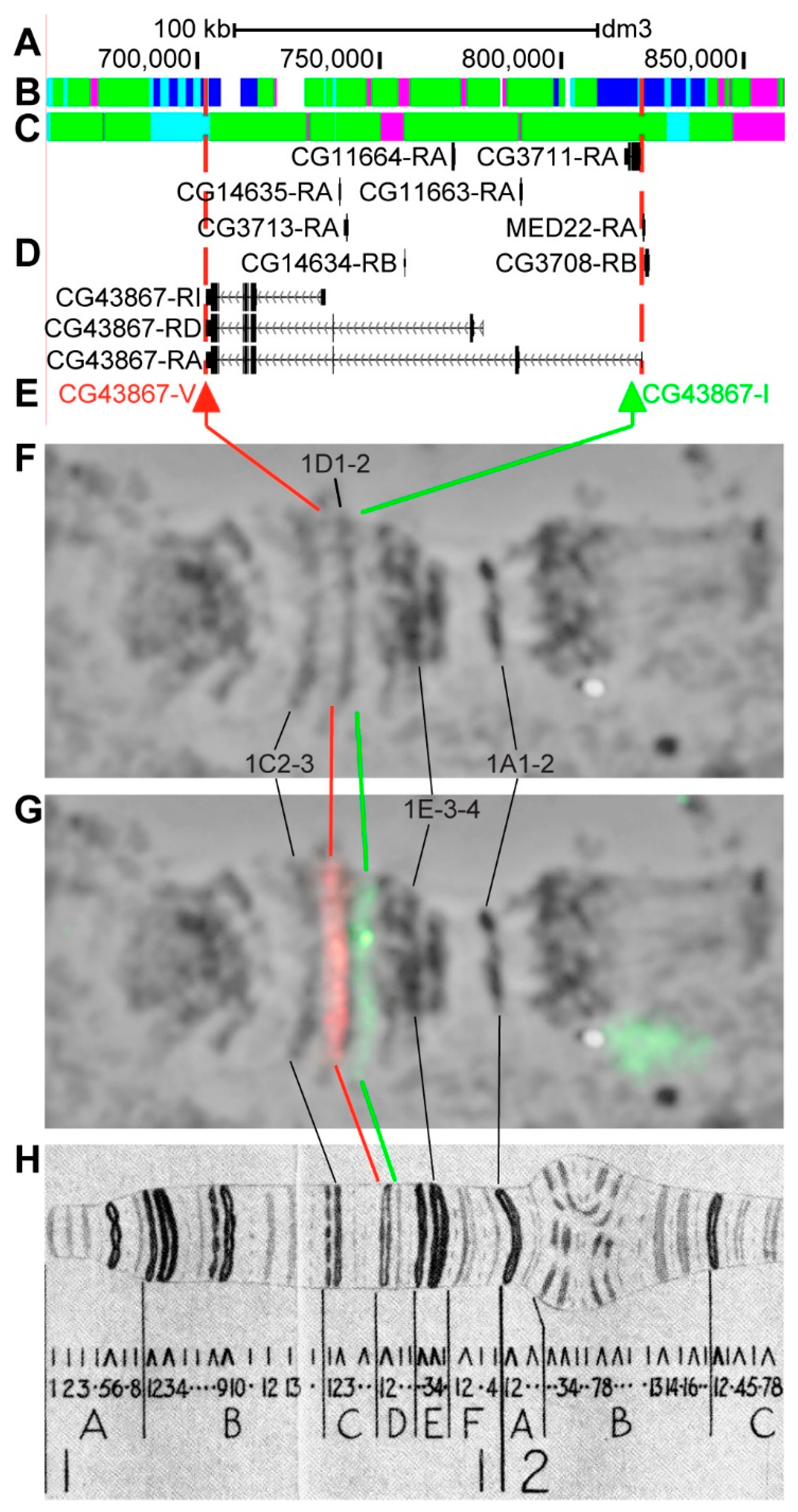
3.2.2. CG43867
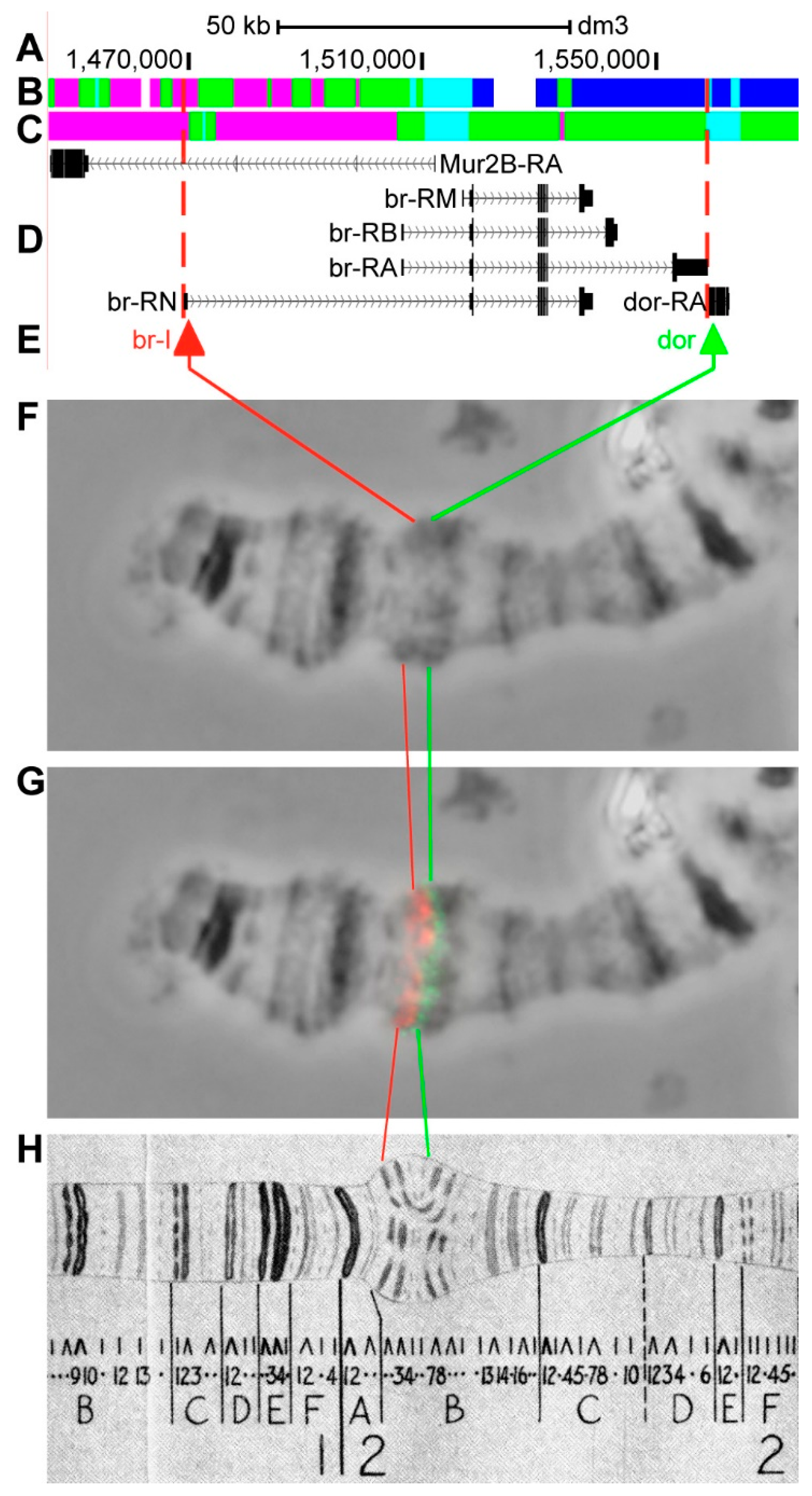
3.2.3. br
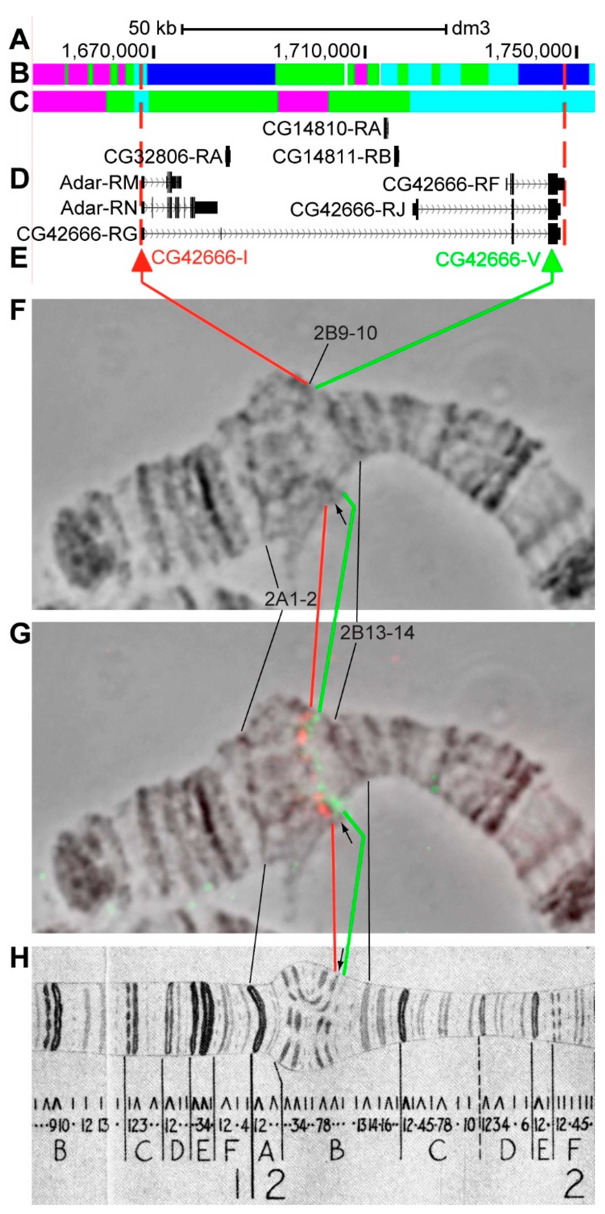
3.2.4. CG42666
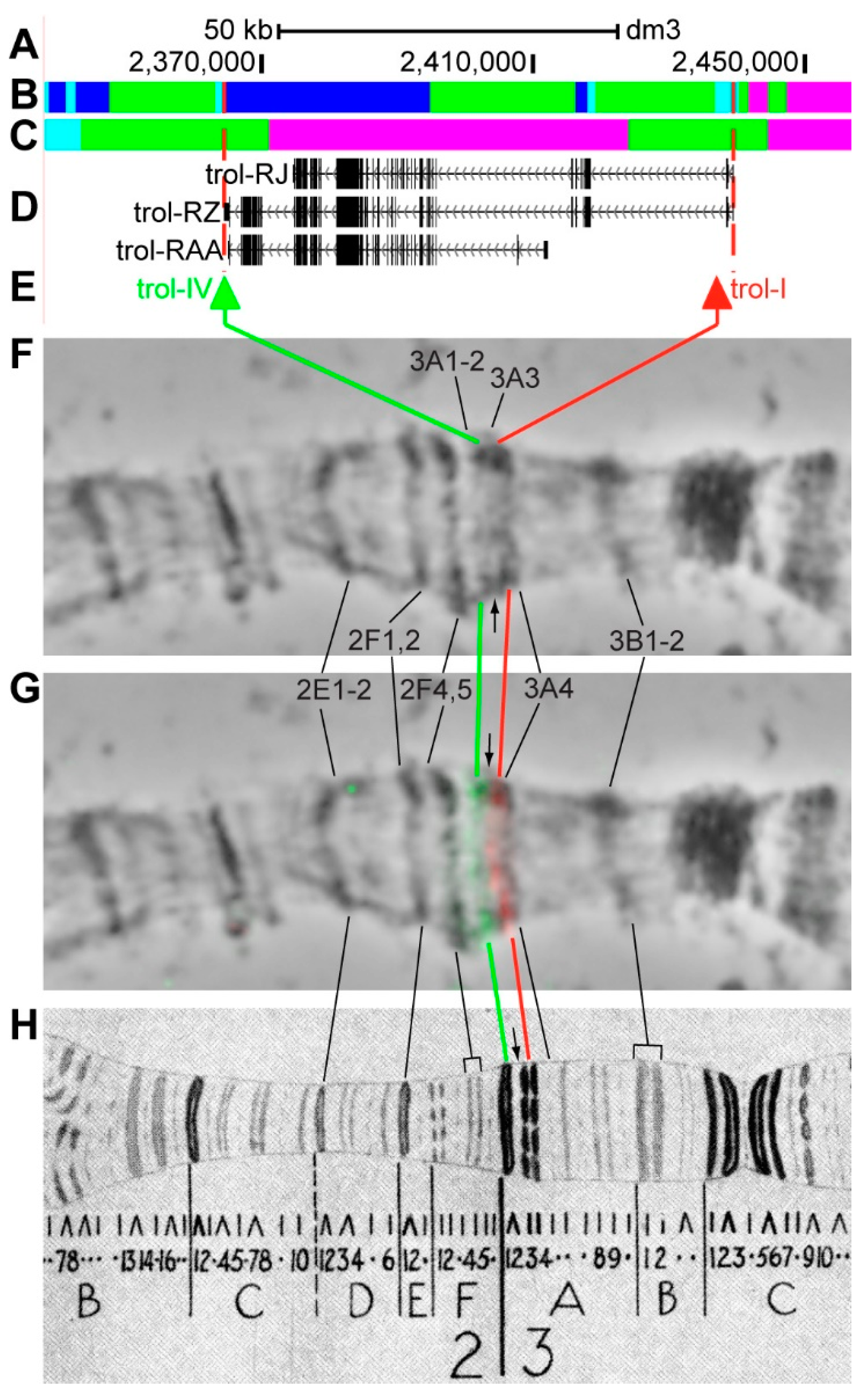
3.2.5. trol
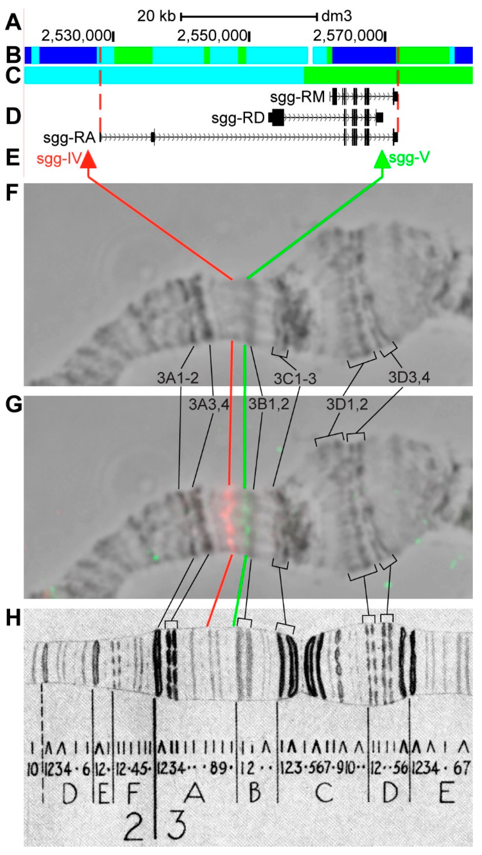
3.2.6. sgg
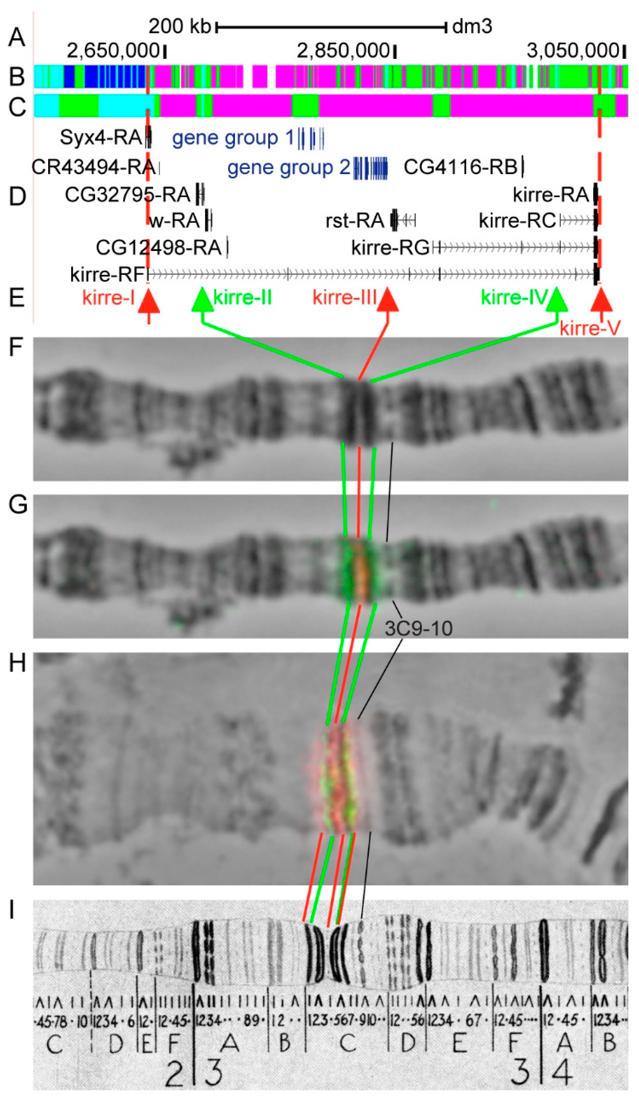
3.2.7. kirre
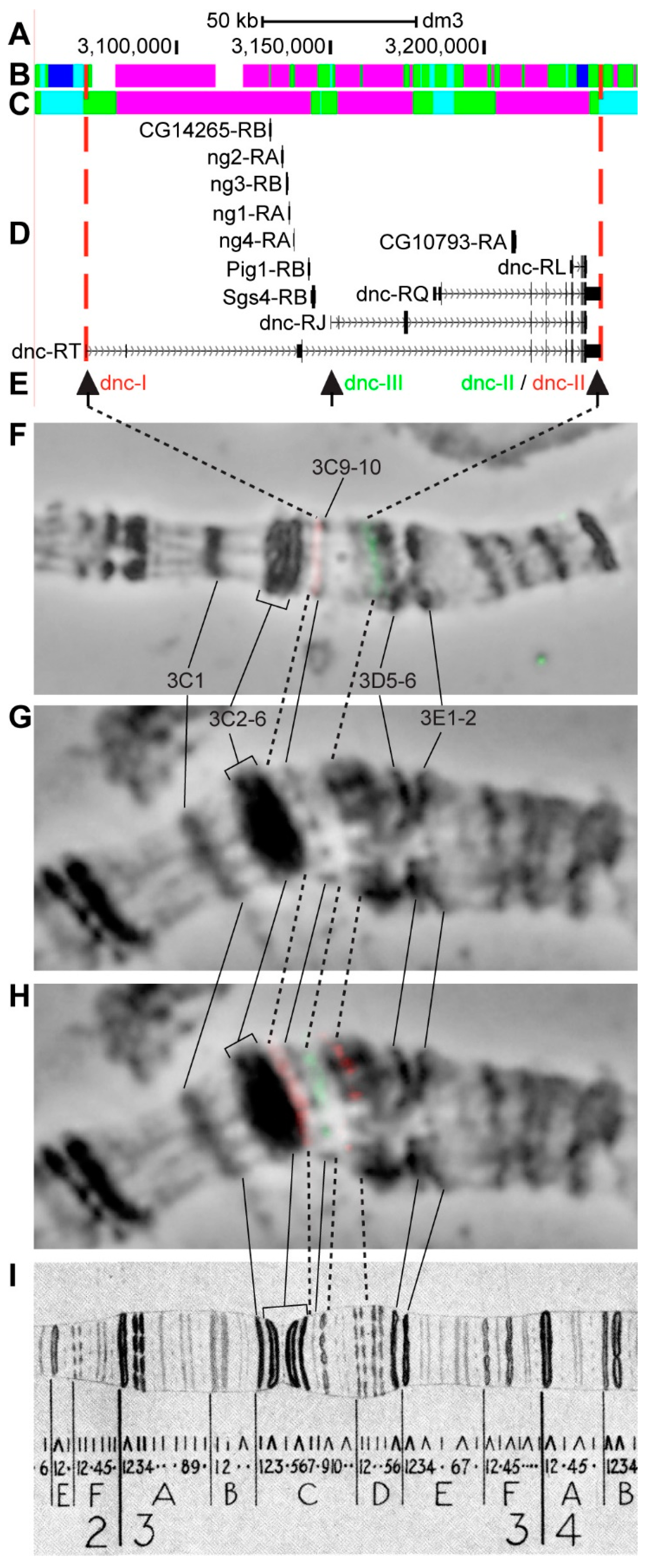
3.2.8. dnc
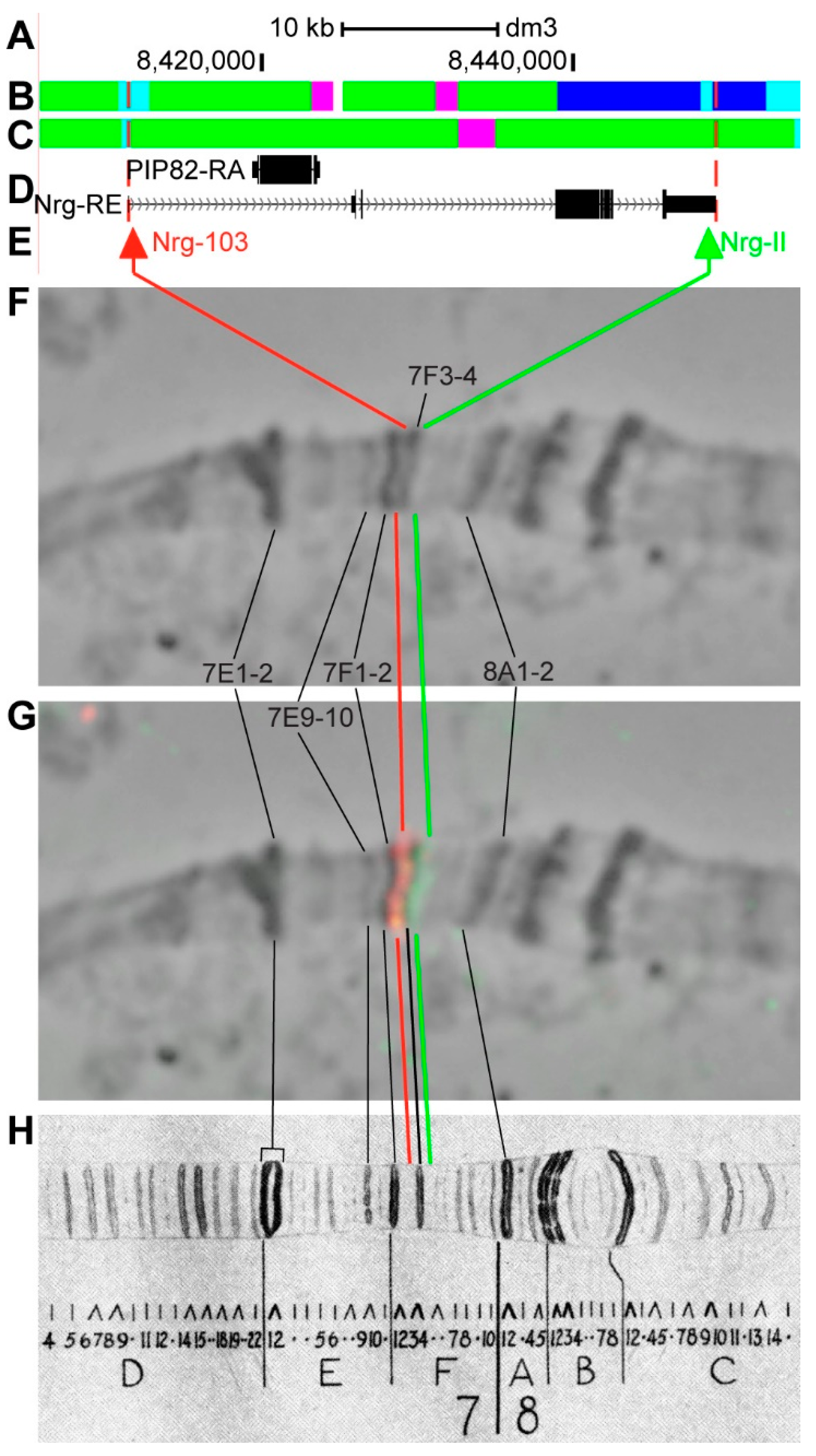
3.2.9. Nrg
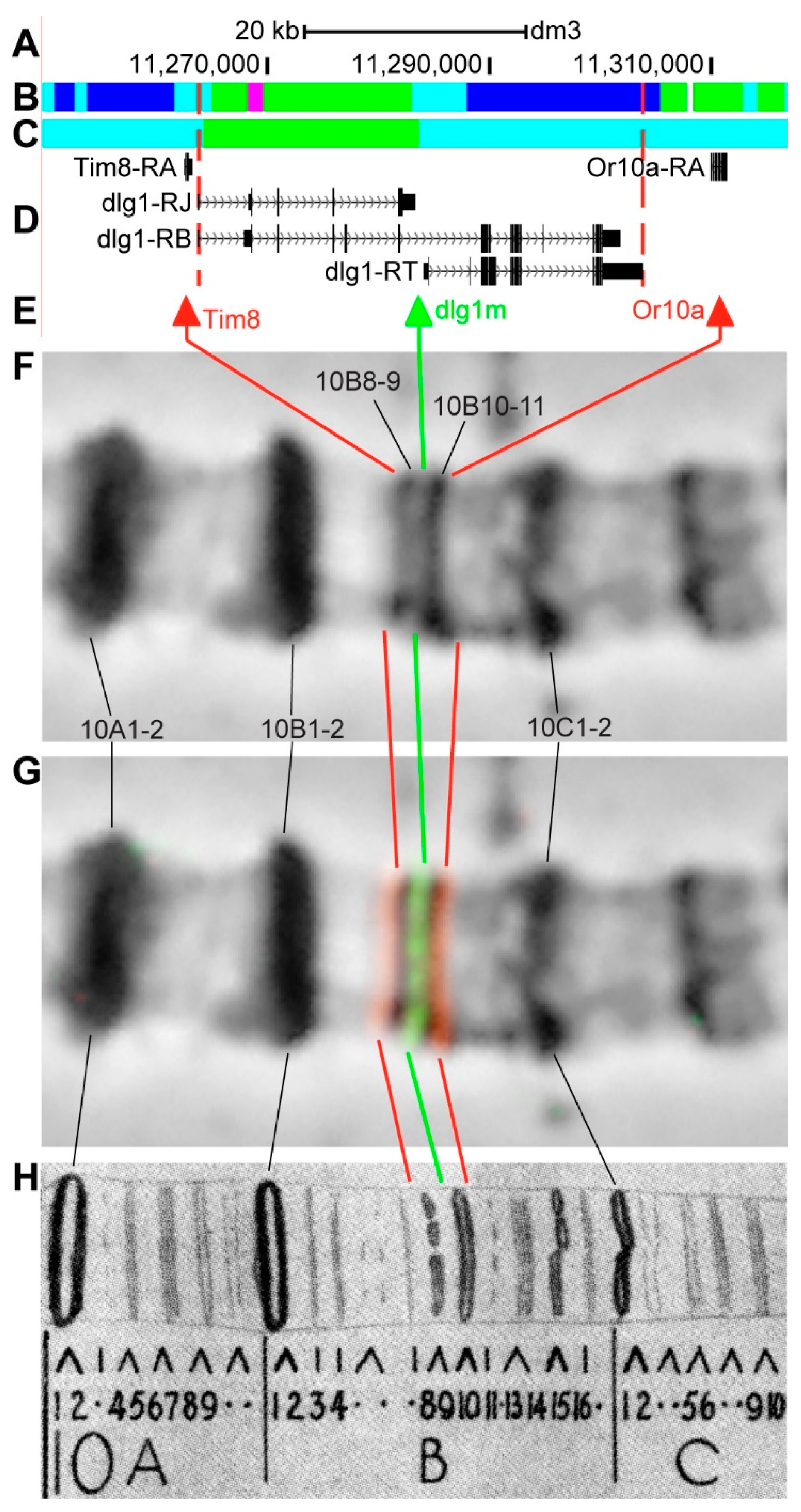
3.2.10. dlg1
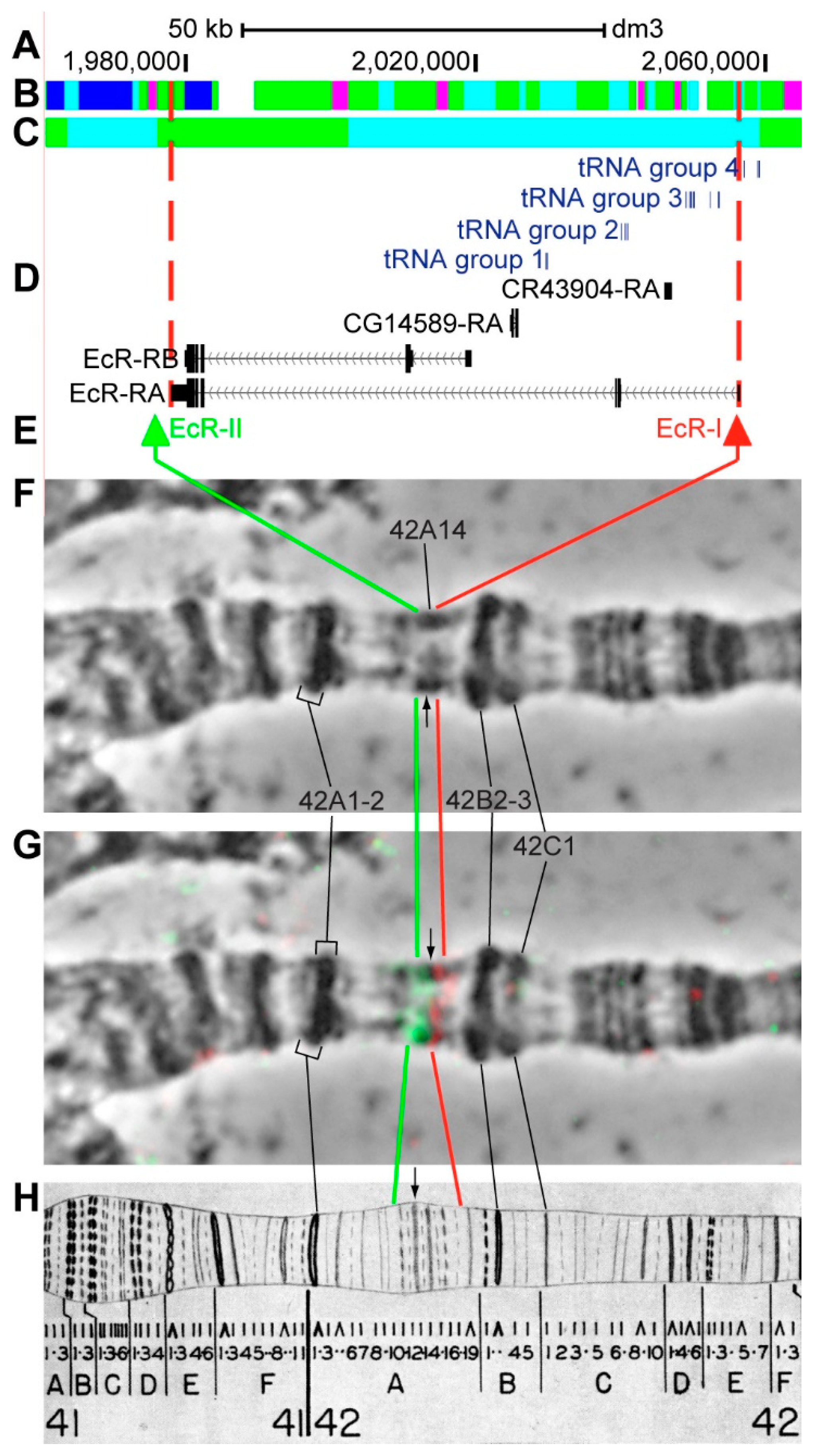
3.2.11. EcR
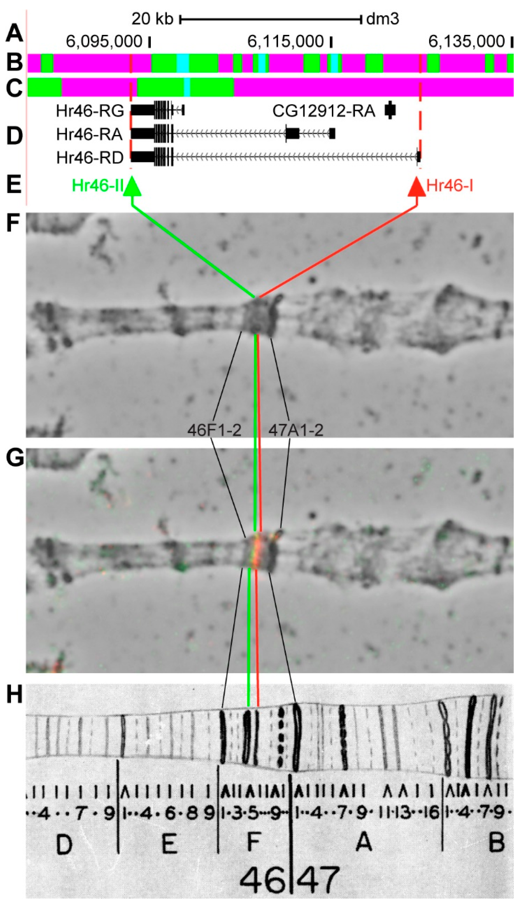
3.2.12. Hr46
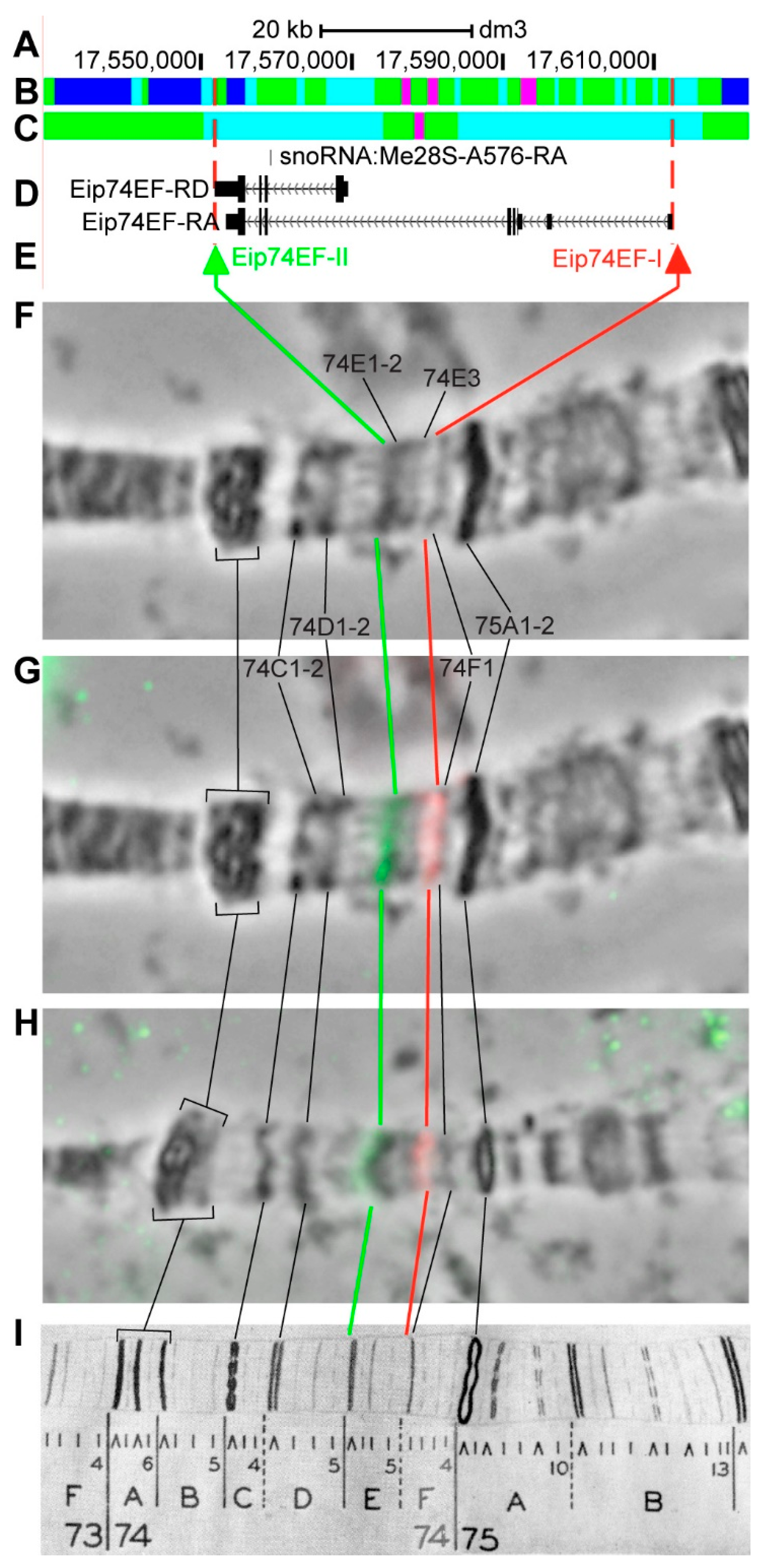
3.2.13. Eip74EF
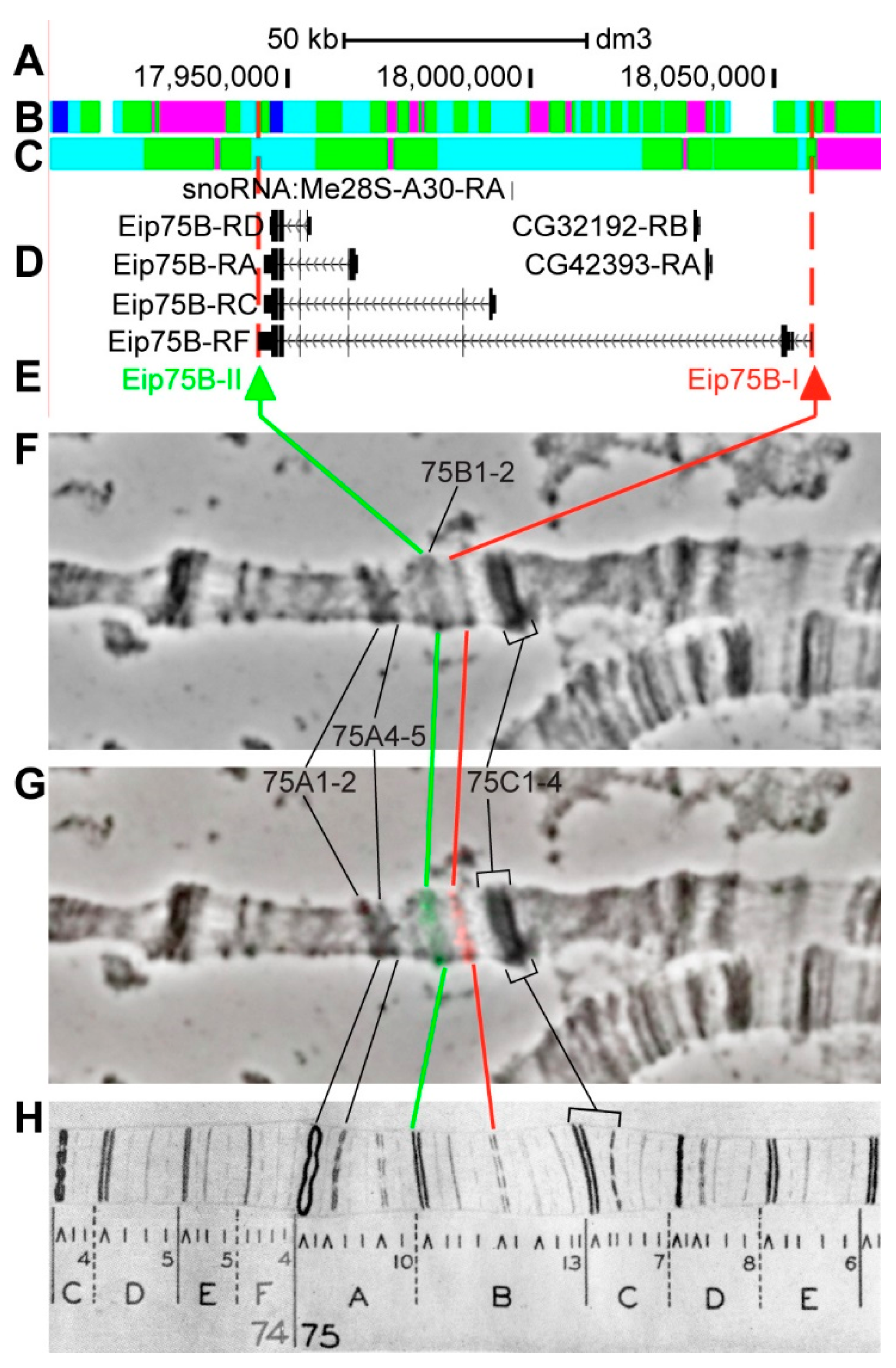
3.2.14. Eip75B
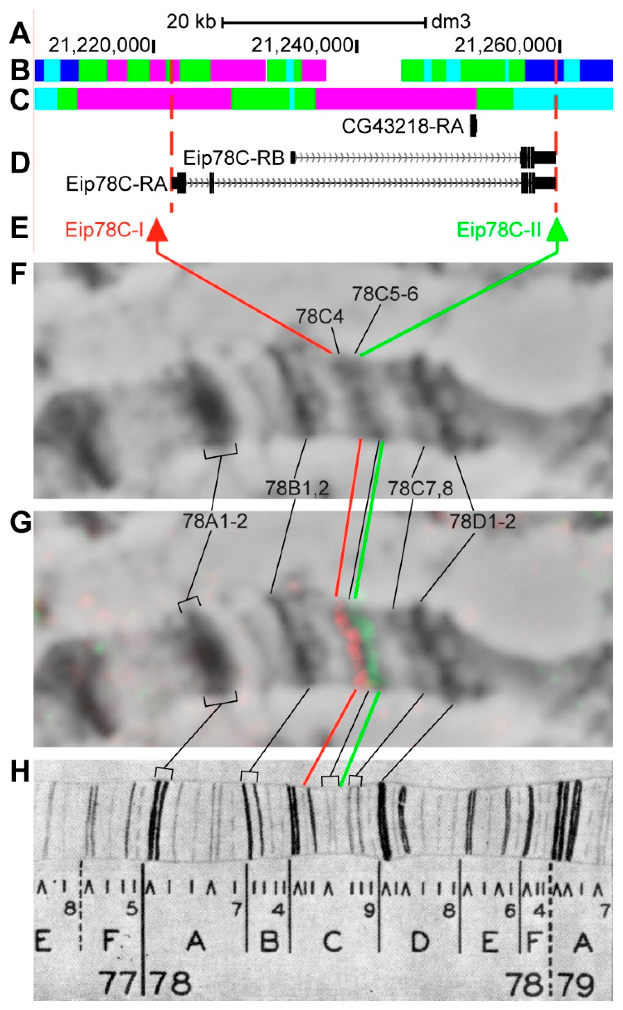
3.2.15. Eip78C
4. Discussion
Supplementary Materials
Author Contributions
Funding
Acknowledgments
Conflicts of Interest
References
- Koltzoff, N. The structure of the chromosomes in the salivary glands of Drosophila. Science 1934, 80, 312–313. [Google Scholar] [CrossRef] [PubMed]
- Mackensen, O. Locating genes on the salivary chromosomes. Cytogenetic methods demonstrated in determining position of genes on the X-chromosome of Drosophila melanogaster. J. Hered. 1935, 26, 163–174. [Google Scholar] [CrossRef]
- Muller, H.J.; Prokofyeva, A.A. The individual gene in relation to the chromomere and the chromosome. Proc. Natl. Acad. Sci. USA 1935, 21, 16–26. [Google Scholar] [CrossRef]
- Bridges, C.B. Salivary chromosome maps: With a key to the banding of the chromosomes of Drosophila melanogaster. J. Hered. 1935, 26, 60–64. [Google Scholar] [CrossRef]
- Muller, H.J. On the dimensions of chromosomes and genes in Drosophila salivary glands. Am. Nat. 1935, 69, 405–411. [Google Scholar] [CrossRef]
- Prokofyeva-Belgovskaya, A.A. The structure of the chromocenter. Cytologia 1935, 6, 438–443. [Google Scholar] [CrossRef]
- Metz, C.W. Effects of mechanical distortion on the structure of salivary gland chromosomes. Biol. Bull. 1936, 71, 238–248. [Google Scholar] [CrossRef]
- Animal Cytology and Evolution, 2nd ed.; Cambridge University Press: Cambridge, UK, 1954.
- Bauer, H.; Beermann, W. Polytenia of giant chromosomes. Chromosoma 1952, 4, 830–848. [Google Scholar]
- Beermann, W. Chromomore constancy and specific modifications of the chromosome structure in development and organ differentiation of Chironomus tentans. Chromosoma 1952, 5, 139–198. [Google Scholar] [CrossRef]
- Beermann, W. Nuclear differentiation and functional morphology of chromosomes. Cold Spring Harb. Symp. Quant. Biol. 1956, 21, 217–232. [Google Scholar] [CrossRef]
- Mechelke, F. Reversible structural modifications of the chromosomes in salivary glands of Acricotopus lucidus. Chromosoma 1953, 5, 511–543. [Google Scholar] [CrossRef] [PubMed]
- Breuer, M.E.; Pavan, C. Behavior of polytene chromosomes of Rhynchosciara angelae at different stages of larval development. Chromosoma 1955, 7, 341–386. [Google Scholar] [CrossRef] [PubMed]
- Beermann, W. Structure and function of interphase chromosomes. In Genetics Today: XI International Congress of Genetics; Pergamon Press: Oxford, UK; London, UK; Edinburgh, Scotland; New York, NY, USA; Paris, France; Frankfurt, Germany, 1965; Volume 2, pp. 375–384. [Google Scholar]
- Beermann, W. Gene action at the level of the chromosome. In Heritage from Mendel; The University of Wisconsin Press: Madison, WI, USA; London, UK, 1967; pp. 179–201. [Google Scholar]
- Rudkin, G.T. The relative mutabilities of DNA in regions of the X chromosome of Drosophila melanogaster. Genetics 1965, 52, 665–681. [Google Scholar] [PubMed]
- Olenov, I.M. Genome organization in Metazoa. Tsitologiya 1974, 16, 403–419. [Google Scholar]
- Judd, B.H.; Shen, M.W.; Kaufman, T.C. The anatomy and function of a segment of the X chromosome of Drosophila melanogaster. Genetics 1972, 71, 139–156. [Google Scholar]
- Zhimulev, I.F. Genetic Organization of Polytene Chromosomes, 1st ed.; Academic Press: Cambridge, MA, USA, 1999; Volume 39, ISBN 0-12-017639-4. [Google Scholar]
- Crick, F. General model for the chromosomes of higher organisms. Nature 1971, 234, 25–27. [Google Scholar] [CrossRef]
- Paul, J. General theory of chromosome structure and gene activation in eukaryotes. Nature 1972, 238, 444–446. [Google Scholar] [CrossRef]
- Sorsa, V. Electron microscopic mapping and ultrastructure of Drosophila polytene chromosomes. In Insect Ultrastructure: Volume 2; King, R.C., Akai, H., Eds.; Springer US: Boston, MA, USA, 1984; pp. 75–107. ISBN 978-1-4613-2715-8. [Google Scholar]
- Speiser, C. A hypothesis on the functional organization of the chromosomes of higher organisms. Theor. Appl. Genet. 1974, 44, 97–99. [Google Scholar] [CrossRef]
- Zhimulev, I.F.; Belyaeva, E.S. Proposals to the problem of structural and functional organization of polytene chromosomes. Theor. Appl. Genet. 1974, 45, 335–340. [Google Scholar] [CrossRef]
- Bridges, C.B. A revised map of the salivary gland X-chromosome of Drosophila melanogaster. J. Hered. 1938, 29, 11–13. [Google Scholar] [CrossRef]
- Kozlova, T.Y.; Semeshin, V.F.; Tretyakova, I.V.; Kokoza, E.B.; Pirrotta, V.; Grafodatskaya, V.E.; Belyaeva, E.S.; Zhimulev, I.F. Molecular and cytogenetical characterization of the 10A1-2 band and adjoining region in the Drosophila melanogaster polytene X chromosome. Genetics 1994, 136, 1063–1073. [Google Scholar] [PubMed]
- Vatolina, T.Y.; Boldyreva, L.V.; Demakova, O.V.; Demakov, S.A.; Kokoza, E.B.; Semeshin, V.F.; Babenko, V.N.; Goncharov, F.P.; Belyaeva, E.S.; Zhimulev, I.F. Identical functional organization of nonpolytene and polytene chromosomes in Drosophila melanogaster. PLoS ONE 2011, 6, e25960. [Google Scholar] [CrossRef]
- Adams, M.D.; Celniker, S.E.; Holt, R.A.; Evans, C.A.; Gocayne, J.D.; Amanatides, P.G.; Scherer, S.E.; Li, P.W.; Hoskins, R.A.; Galle, R.F.; et al. The genome sequence of Drosophila melanogaster. Science 2000, 287, 2185–2195. [Google Scholar] [CrossRef] [PubMed]
- modENCODE Consortium; Roy, S.; Ernst, J.; Kharchenko, P.V.; Kheradpour, P.; Negre, N.; Eaton, M.L.; Landolin, J.M.; Bristow, C.A.; Ma, L.; et al. Identification of functional elements and regulatory circuits by Drosophila modENCODE. Science 2010, 330, 1787–1797. [Google Scholar] [PubMed]
- Filion, G.J.; van Bemmel, J.G.; Braunschweig, U.; Talhout, W.; Kind, J.; Ward, L.D.; Brugman, W.; de Castro, I.J.; Kerkhoven, R.M.; Bussemaker, H.J.; et al. Systematic protein location mapping reveals five principal chromatin types in Drosophila cells. Cell 2010, 143, 212–224. [Google Scholar] [CrossRef] [PubMed]
- Kharchenko, P.V.; Alekseyenko, A.A.; Schwartz, Y.B.; Minoda, A.; Riddle, N.C.; Ernst, J.; Sabo, P.J.; Larschan, E.; Gorchakov, A.A.; Gu, T.; et al. Comprehensive analysis of the chromatin landscape in Drosophila melanogaster. Nature 2011, 471, 480–485. [Google Scholar] [CrossRef] [PubMed]
- Milon, B.; Sun, Y.; Chang, W.; Creasy, T.; Mahurkar, A.; Shetty, A.; Nurminsky, D.; Nurminskaya, M. Map of open and closed chromatin domains in Drosophila genome. BMC Genom. 2014, 15, 988. [Google Scholar] [CrossRef]
- Demakova, O.V.; Demakov, S.A.; Boldyreva, L.V.; Zykova, T.Y.; Levitsky, V.G.; Semeshin, V.F.; Pokholkova, G.V.; Sidorenko, D.S.; Goncharov, F.P.; Belyaeva, E.S.; et al. Faint gray bands in Drosophila melanogaster polytene chromosomes are formed by coding sequences of housekeeping genes. Chromosoma 2019, 129, 25–44. [Google Scholar] [CrossRef]
- Sidorenko, D.S.; Sidorenko, I.A.; Zykova, T.Y.; Goncharov, F.P.; Larsson, J.; Zhimulev, I.F. Molecular and genetic organization of bands and interbands in the dot chromosome of Drosophila melanogaster. Chromosoma 2019, 128, 97–117. [Google Scholar] [CrossRef]
- Semeshin, V.F.; Demakov, S.A.; Zhimulev, I.F. Characteristics of structures of Drosophila polytene chromosomes formed by transposable DNA fragments. Genetika 1989, 25, 1968–1978. [Google Scholar]
- Demakov, S.A.; Vatolina, T.Y.; Babenko, V.N.; Semeshin, V.F.; Belyaeva, E.S.; Zhimulev, I.F. Protein composition of interband regions in polytene and cell line chromosomes of Drosophila melanogaster. BMC Genom. 2011, 12, 566. [Google Scholar] [CrossRef] [PubMed]
- Zhimulev, I.F.; Belyaeva, E.S.; Vatolina, T.Y.; Demakov, S.A. Banding patterns in Drosophila melanogaster polytene chromosomes correlate with DNA-binding protein occupancy. Bioessays 2012, 34, 498–508. [Google Scholar] [CrossRef] [PubMed]
- Boldyreva, L.V.; Goncharov, F.P.; Demakova, O.V.; Zykova, T.Y.; Levitsky, V.G.; Kolesnikov, N.N.; Pindyurin, A.V.; Semeshin, V.F.; Zhimulev, I.F. Protein and genetic composition of four chromatin types in Drosophila melanogaster cell lines. Curr. Genom. 2017, 18, 214–226. [Google Scholar] [CrossRef] [PubMed]
- Zhimulev, I.F.; Zykova, T.Y.; Goncharov, F.P.; Khoroshko, V.A.; Demakova, O.V.; Semeshin, V.F.; Pokholkova, G.V.; Boldyreva, L.V.; Demidova, D.S.; Babenko, V.N.; et al. Genetic organization of interphase chromosome bands and interbands in Drosophila melanogaster. PLoS ONE 2014, 9, e101631. [Google Scholar] [CrossRef] [PubMed]
- Zykova, T.Y.; Levitsky, V.G.; Belyaeva, E.S.; Zhimulev, I.F. Polytene chromosomes—A portrait of functional organization of the Drosophila genome. Curr. Genom. 2018, 19, 179–191. [Google Scholar] [CrossRef] [PubMed]
- Zykova, T.Y.; Popova, O.O.; Khoroshko, V.A.; Levitsky, V.G.; Lavrov, S.A.; Zhimulev, I.F. Genetic organization of open chromatin domains situated in polytene chromosome interbands in Drosophila. Dokl. Biochem. Biophys. 2018, 483, 297–301. [Google Scholar] [CrossRef] [PubMed]
- Khoroshko, V.A.; Levitsky, V.G.; Zykova, T.Y.; Antonenko, O.V.; Belyaeva, E.S.; Zhimulev, I.F. Chromatin heterogeneity and distribution of regulatory elements in the late-replicating intercalary heterochromatin domains of Drosophila melanogaster chromosomes. PLoS ONE 2016, 11, e0157147. [Google Scholar] [CrossRef]
- Beermann, W. Chromomeres and genes. Results Probl. Cell Differ. 1972, 4, 1–33. [Google Scholar]
- Semeshin, V.F.; Demakov, S.A.; Perez Alonso, M.; Belyaeva, E.S.; Bonner, J.J.; Zhimulev, I.F. Electron microscopical analysis of Drosophila polytene chromosomes. V. Characteristics of structures formed by transposed DNA segments of mobile elements. Chromosoma 1989, 97, 396–412. [Google Scholar] [CrossRef]
- Khoroshko, V.A.; Pokholkova, G.V.; Zykova, T.Y.; Osadchiy, I.S.; Zhimulev, I.F. Gene dunce localization in the polytene chromosome of Drosophila melanogaster long span batch of adjacent chromosomal structures. Dokl. Biochem. Biophys. 2019, 484, 55–58. [Google Scholar] [CrossRef]
- Zhimulev, I.F.; Boldyreva, L.V.; Demakova, O.V.; Poholkova, G.V.; Khoroshko, V.A.; Zykova, T.Y.; Lavrov, S.A.; Belyaeva, E.S. Drosophila polytene chromosome bands formed by gene introns. Dokl. Biochem. Biophys. 2016, 466, 57–60. [Google Scholar] [CrossRef] [PubMed]
- Semeshin, V.F.; Belyaeva, E.S.; Shloma, V.V.; Zhimulev, I.F. Electron microscopy of polytene chromosomes. Methods Mol. Biol. 2004, 247, 305–324. [Google Scholar] [PubMed]
- Ashburner, M.; Golic, K.G.; Hawley, R.S. Drosophila: A Laboratory Handbook, 2nd ed.; Cold Spring Harbor Laboratory Press: Cold Spring Harbor, NY, USA, 2005; ISBN 0-87969-706-7. [Google Scholar]
- Machyna, M.; Kiefer, L.; Simon, M.D. Enhanced nucleotide chemistry and toehold nanotechnology reveals lncRNA spreading on chromatin. Nat. Struct. Mol. Biol. 2020, 27, 297–304. [Google Scholar] [CrossRef] [PubMed]
- Belyaeva, E.S.; Vlassova, I.E.; Biyasheva, Z.M.; Kakpakov, V.T.; Richards, G.; Zhimulev, I.F. Cytogenetic analysis of the 2B3-4-2B11 region of the X chromosome of Drosophila melanogaster. II. Changes in 20-OH ecdysone puffing caused by genetic defects of puff 2B5. Chromosoma 1981, 84, 207–219. [Google Scholar] [CrossRef] [PubMed]
- Belyaeva, E.S.; Protopopov, M.O.; Baricheva, E.M.; Semeshin, V.F.; Izquierdo, M.L.; Zhimulev, I.F. Cytogenetic analysis of region 2B3-4—2B11 of the X-chromosome of Drosophila melanogaster. VI. Molecular and cytological mapping the ecs locus and the 2B puff. Chromosoma 1987, 95, 295–310. [Google Scholar] [CrossRef]
- DiBello, P.R.; Withers, D.A.; Bayer, C.A.; Fristrom, J.W.; Guild, G.M. The Drosophila Broad-Complex encodes a family of related proteins containing zinc fingers. Genetics 1991, 129, 385–397. [Google Scholar]
- Bayer, C.A.; Holley, B.; Fristrom, J.W. A switch in Broad-Complex zinc-finger isoform expression is regulated posttranscriptionally during the metamorphosis of Drosophila imaginal discs. Dev. Biol. 1996, 177, 1–14. [Google Scholar] [CrossRef]
- Belyaeva, E.S.; Zhimulev, I.F. Cytogenetic analysis of the X-chromosome region 2B3-4—2B11 of Drosophila melanogaster. IV. Mutation at the swi (singed wings) locus interfering with the late 20-OH ecdysone puff system. Chromosoma 1982, 86, 251–263. [Google Scholar] [CrossRef]
- Bridges, C.B.; Bridges, P.N. A new map of the second chromosome: A revised map of the right limb of the second chromosome of Drosophila melanogaster. J. Hered. 1939, 30, 475–476. [Google Scholar] [CrossRef]
- Semeshin, V.F.; Baricheva, E.M.; Belyaeva, E.S.; Zhimulev, I.F. Electron microscopical analysis of Drosophila polytene chromosomes. II. Development of complex puffs. Chromosoma 1985, 91, 210–233. [Google Scholar] [CrossRef]
- Bridges, P.N. A revised map of the left limb of the third chromosome of Drosophila melanogaster. J. Hered. 1941, 32, 64–65. [Google Scholar] [CrossRef]
- Zhimulev, I.F.; Belyaeva, E.S. 3H-Uridine labelling patterns in the Drosophila melanogaster salivary gland chromosomes X, 2R and 3L. Chromosoma 1975, 49, 219–231. [Google Scholar] [CrossRef]
- Arcos-Terán, L. DNA replication and the nature of late replicating loci in the X-chromosome of Drosophila melanogaster. Chromosoma 1972, 37, 233–296. [Google Scholar] [CrossRef] [PubMed]
- Zhimulev, I.F.; Belyaeva, E.S.; Makunin, I.V.; Pirrotta, V.; Volkova, E.I.; Alekseyenko, A.A.; Andreyeva, E.N.; Makarevich, G.F.; Boldyreva, L.V.; Nanayev, R.A.; et al. Influence of the SuUR gene on intercalary heterochromatin in Drosophila melanogaster polytene chromosomes. Chromosoma 2003, 111, 377–398. [Google Scholar] [CrossRef] [PubMed]
- Rykowski, M.C.; Parmelee, S.J.; Agard, D.A.; Sedat, J.W. Precise determination of the molecular limits of a polytene chromosome band: Regulatory sequences for the Notch gene are in the interband. Cell 1988, 54, 461–472. [Google Scholar] [CrossRef]
- Volkova, E.I.; Andreyenkova, N.G.; Andreyenkov, O.V.; Sidorenko, D.S.; Zhimulev, I.F.; Demakov, S.A. Structural and functional dissection of the 5’ region of the Notch gene in Drosophila melanogaster. Genes (Basel) 2019, 10, 1037. [Google Scholar] [CrossRef]
- White, K.P.; Hurban, P.; Watanabe, T.; Hogness, D.S. Coordination of Drosophila metamorphosis by two ecdysone-induced nuclear receptors. Science 1997, 276, 114–117. [Google Scholar] [CrossRef]
- Bender, M.; Imam, F.B.; Talbot, W.S.; Ganetzky, B.; Hogness, D.S. Drosophila ecdysone receptor mutations reveal functional differences among receptor isoforms. Cell 1997, 91, 777–788. [Google Scholar] [CrossRef]
- Schwaiger, M.; Stadler, M.B.; Bell, O.; Kohler, H.; Oakeley, E.J.; Schübeler, D. Chromatin state marks cell-type- and gender-specific replication of the Drosophila genome. Genes Dev. 2009, 23, 589–601. [Google Scholar] [CrossRef]
- Braunschweig, U.; Hogan, G.J.; Pagie, L.; van Steensel, B. Histone H1 binding is inhibited by histone variant H3. 3. EMBO J. 2009, 28, 3635–3645. [Google Scholar] [CrossRef]
- Eaton, M.L.; Prinz, J.A.; MacAlpine, H.K.; Tretyakov, G.; Kharchenko, P.V.; MacAlpine, D.M. Chromatin signatures of the Drosophila replication program. Genome Res. 2011, 21, 164–174. [Google Scholar] [CrossRef] [PubMed]
- Sher, N.; Bell, G.W.; Li, S.; Nordman, J.; Eng, T.; Eaton, M.L.; MacAlpine, D.M.; Orr-Weaver, T.L. Developmental control of gene copy number by repression of replication initiation and fork progression. Genome Res. 2012, 22, 64–75. [Google Scholar] [CrossRef] [PubMed]


| Gene | Gene Location According to UCSC | Gene Size, kb | Intron Size, % |
|---|---|---|---|
| CG3777 | 1A1–1A5 | 70.6 | 95.2 |
| CG43867 | 1C5–1D2 | 119.7 | 94.2 |
| br (broad) | 2B3–2B4 | 70 | 93.5 |
| CG42666 (or prage) | 2B9–2B12 | 79.2 | 96.3 |
| trol (terribly reduced optic lobes) | 3A3–3A4 | 74.9 | 81.9 |
| sgg (shaggy) | 3A8–3B1 | 43.8 | 93.3 |
| kirre (kin of irre) | 3B4–3C7 | 393.7 | 98.4 |
| dnc (dunce) | 3C9–3D1 | 167.3 | 94.8 |
| Nrg (Neuroglian) | 7F2–7F4 | 37.7 | 80.4 |
| dlg1 (discs large 1) | 10B6–10B10 | 40.1 | 81.9 |
| EcR (Ecdysone receptor) | 42A9–42A12 | 78.6 | 93.5 |
| Hr46 (Hormone receptor-like in 46 or Hormone receptor 3) | 46F5–46F7 | 31.8 | 86.7 |
| Eip74EF (Ecdysone-induced protein 74EF) | 74D4–74E2 | 59.1 | 89.8 |
| Eip75B (Ecdysone-induced protein 75B) | 75A10–75B6 | 113.7 | 94.8 |
| Eip78C (Ecdysone-induced protein 78C) | 78C2–78C3 | 39.5 | 86.8 |
© 2020 by the authors. Licensee MDPI, Basel, Switzerland. This article is an open access article distributed under the terms and conditions of the Creative Commons Attribution (CC BY) license (http://creativecommons.org/licenses/by/4.0/).
Share and Cite
Khoroshko, V.A.; Pokholkova, G.V.; Levitsky, V.G.; Zykova, T.Y.; Antonenko, O.V.; Belyaeva, E.S.; Zhimulev, I.F. Genes Containing Long Introns Occupy Series of Bands and Interbands in Drosophila melanogaster Polytene Chromosomes. Genes 2020, 11, 417. https://doi.org/10.3390/genes11040417
Khoroshko VA, Pokholkova GV, Levitsky VG, Zykova TY, Antonenko OV, Belyaeva ES, Zhimulev IF. Genes Containing Long Introns Occupy Series of Bands and Interbands in Drosophila melanogaster Polytene Chromosomes. Genes. 2020; 11(4):417. https://doi.org/10.3390/genes11040417
Chicago/Turabian StyleKhoroshko, Varvara A., Galina V. Pokholkova, Victor G. Levitsky, Tatyana Yu. Zykova, Oksana V. Antonenko, Elena S. Belyaeva, and Igor F. Zhimulev. 2020. "Genes Containing Long Introns Occupy Series of Bands and Interbands in Drosophila melanogaster Polytene Chromosomes" Genes 11, no. 4: 417. https://doi.org/10.3390/genes11040417
APA StyleKhoroshko, V. A., Pokholkova, G. V., Levitsky, V. G., Zykova, T. Y., Antonenko, O. V., Belyaeva, E. S., & Zhimulev, I. F. (2020). Genes Containing Long Introns Occupy Series of Bands and Interbands in Drosophila melanogaster Polytene Chromosomes. Genes, 11(4), 417. https://doi.org/10.3390/genes11040417