
Strategies to Increase Prediction Accuracy in Genomic Selection of Complex Traits in Alfalfa (Medicago sativa L.)


Abstract
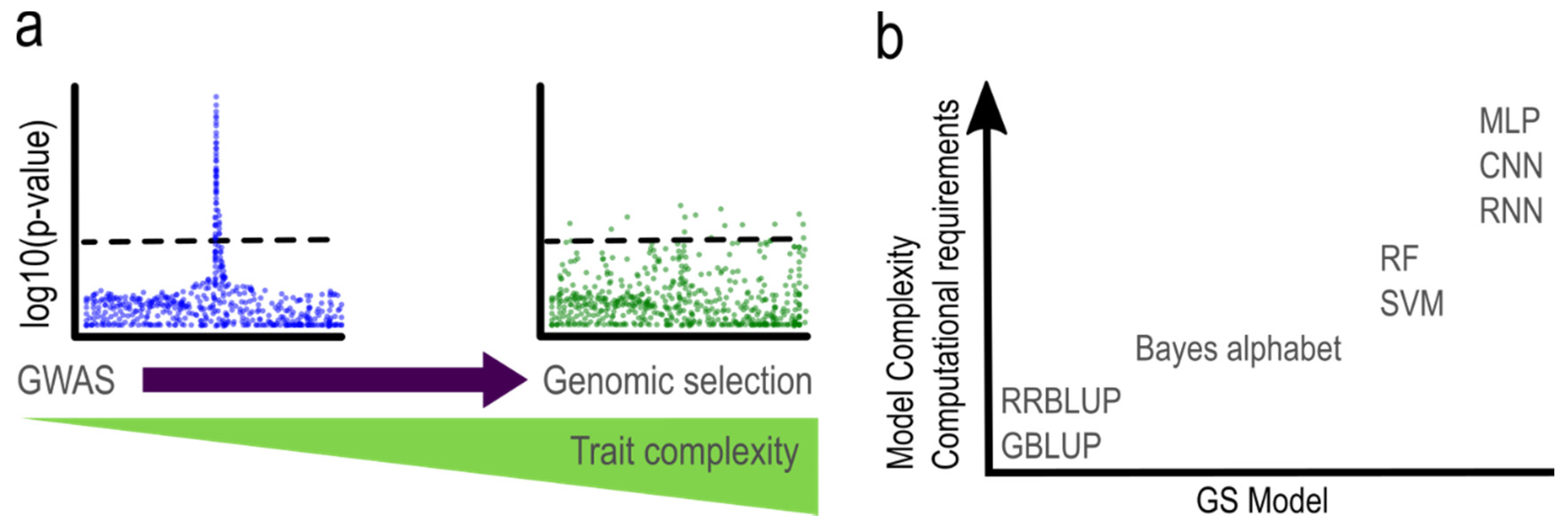
:1. Introduction
2. Statistical Methods in GS
2.1. Ridge-Regression Best Linear Unbiased Prediction (RRBLUP)
2.2. Genomic Best Linear Unbiased Prediction (GBLUP)
Weighted Genomic Best Linear Unbiased Prediction (WGBLUP)
2.3. Bayesian Models
2.4. Machine Learning Models
2.4.1. Support Vector Machine (SVM)
2.4.2. Random Forest (RF)
2.4.3. Deep Learning (DL)
2.5. Other Models
3. Genomic Selection in Polyploids
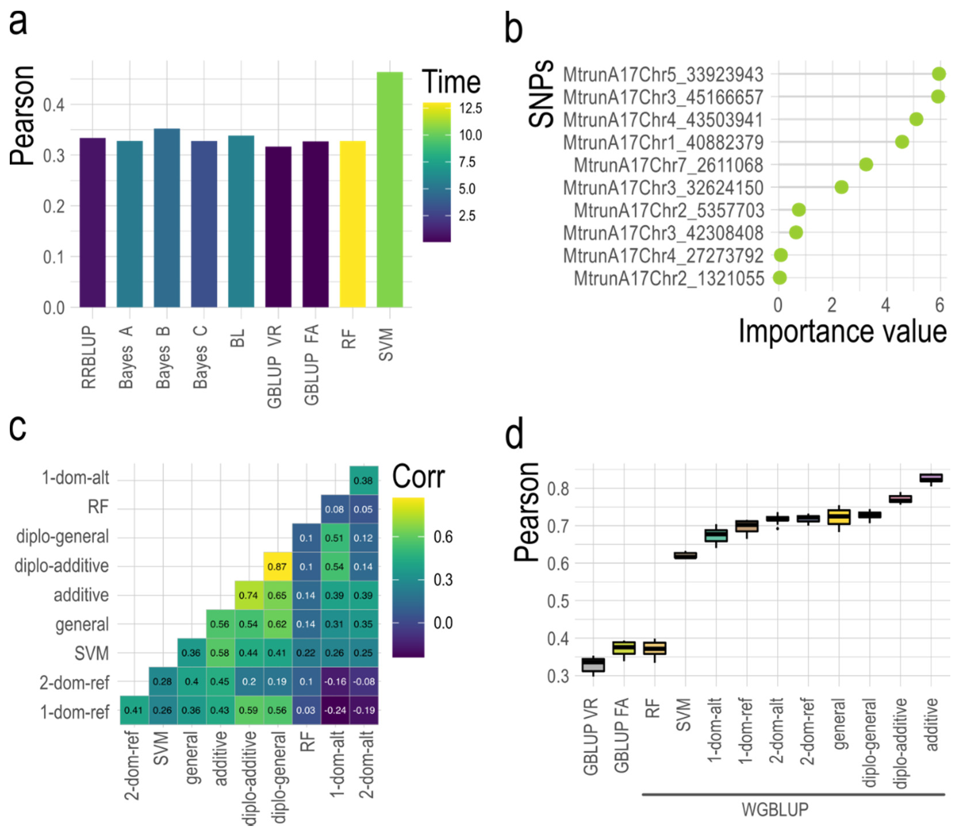
4. Case Study: Logan 2020 Population
5. Case Study: Potato Diversity Panel
6. Conclusions
Author Contributions
Funding
Institutional Review Board Statement
Informed Consent Statement
Data Availability Statement
Acknowledgments
Conflicts of Interest
References
- Blondon, F.; Marie, D.; Brown, S.; Kondorosi, A. Genome size and base composition in Medicago sativa and M. truncatula species. Genome 1994, 37, 264–270. [Google Scholar] [CrossRef]
- Elshire, R.J.; Glaubitz, J.C.; Sun, Q.; Poland, J.A.; Kawamoto, K.; Buckler, E.S.; Mitchell, S.E. A Robust, Simple Genotyping-by-Sequencing (GBS) Approach for High Diversity Species. PLoS ONE 2011, 6, e19379. [Google Scholar] [CrossRef] [PubMed] [Green Version]
- Yu, L.-X.; Liu, X.; Boge, W.; Liu, X.-P. Genome-Wide Association Study Identifies Loci for Salt Tolerance during Germination in Autotetraploid Alfalfa (Medicago sativa L.) Using Genotyping-by-Sequencing. Front. Plant Sci. 2016, 7, 956. [Google Scholar] [CrossRef] [Green Version]
- Liu, X.-P.; Yu, L.-X. Genome-Wide Association Mapping of Loci Associated with Plant Growth and Forage Production under Salt Stress in Alfalfa (Medicago sativa L.). Front. Plant Sci. 2017, 8, 853. [Google Scholar] [CrossRef]
- Liu, X.; Hawkins, C.; Peel, M.D.; Yu, L. Genetic Loci Associated with Salt Tolerance in Advanced Breeding Populations of Tetraploid Alfalfa Using Genome-Wide Association Studies. Plant Genome 2019, 12, 180026. [Google Scholar] [CrossRef]
- Medina, C.A.; Hawkins, C.; Liu, X.-P.; Peel, M.; Yu, L.-X. Genome-Wide Association and Prediction of Traits Related to Salt Tolerance in Autotetraploid Alfalfa (Medicago sativa L.). Int. J. Mol. Sci. 2020, 21, 3361. [Google Scholar] [CrossRef]
- Bulmer, M.G. The Effect of Selection on Genetic Variability. Am. Nat. 1971, 105, 201–211. [Google Scholar] [CrossRef]
- Meuwissen, T.H.E.; Hayes, B.J.; Goddard, M.E. Prediction of total genetic value using genome-wide dense marker maps. Genetics 2001, 157, 1819–1829. [Google Scholar] [CrossRef]
- Endelman, J.B. Ridge Regression and Other Kernels for Genomic Selection with R Package rrBLUP. Plant Genome 2011, 4, 250–255. [Google Scholar] [CrossRef] [Green Version]
- Hayes, B.J.; Bowman, P.J.; Chamberlain, A.C.; Verbyla, K.; Goddard, M.E. Accuracy of genomic breeding values in multi-breed dairy cattle populations. Genet. Sel. Evol. 2009, 41, 51. [Google Scholar] [CrossRef] [PubMed] [Green Version]
- Pérez, P.; Campos, G.D.L.; Crossa, J.; Gianola, D. Genomic-Enabled Prediction Based on Molecular Markers and Pedigree Using the Bayesian Linear Regression Package in R. Plant Genome 2010, 3, 106–116. [Google Scholar] [CrossRef]
- Vanraden, P.M. Genomic measures of relationship and inbreeding. Interbull Bull. 2007, 25, 33. [Google Scholar]
- VanRaden, P.M. Efficient Methods to Compute Genomic Predictions. J. Dairy Sci. 2008, 91, 4414–4423. [Google Scholar] [CrossRef] [PubMed] [Green Version]
- Yang, J.; Benyamin, B.; McEvoy, B.P.; Gordon, S.; Henders, A.; Nyholt, D.; Madden, P.A.; Heath, A.C.; Martin, N.; Montgomery, G.; et al. Common SNPs explain a large proportion of the heritability for human height. Nat. Genet. 2010, 42, 565–569. [Google Scholar] [CrossRef] [PubMed] [Green Version]
- Slater, A.T.; Cogan, N.O.; Forster, J.W.; Hayes, B.; Daetwyler, H.D. Improving Genetic Gain with Genomic Selection in Autotetraploid Potato. Plant Genome 2016, 9, 1–15. [Google Scholar] [CrossRef] [PubMed] [Green Version]
- Zhang, Z.; Liu, J.; Ding, X.; Bijma, P.; de Koning, D.-J.; Zhang, Q. Best Linear Unbiased Prediction of Genomic Breeding Values Using a Trait-Specific Marker-Derived Relationship Matrix. PLoS ONE 2010, 5, e12648. [Google Scholar] [CrossRef] [Green Version]
- Legarra, A.; Robert-Granié, C.; Croiseau, P.; Guillaume, F.; Fritz, S. Improved Lasso for genomic selection. Genet. Res. 2010, 93, 77–87. [Google Scholar] [CrossRef] [Green Version]
- Chang, L.-Y.; Toghiani, S.; Hay, E.H.; Aggrey, S.E.; Rekaya, R. A Weighted Genomic Relationship Matrix Based on Fixation Index (FST) Prioritized SNPs for Genomic Selection. Genes 2019, 10, 922. [Google Scholar] [CrossRef] [Green Version]
- Ren, D.; An, L.; Li, B.; Qiao, L.; Liu, W. Efficient weighting methods for genomic best linear-unbiased prediction (BLUP) adapted to the genetic architectures of quantitative traits. Heredity 2020, 126, 320–334. [Google Scholar] [CrossRef]
- Pérez, P.; de los Campos, G. Genome-Wide Regression and Prediction with the BGLR Statistical Package. Genetics 2014, 198, 483–495. [Google Scholar] [CrossRef]
- Meuwissen, T.H.; Solberg, T.R.; Shepherd, R.; Woolliams, J.A. A fast algorithm for BayesB type of prediction of genome-wide estimates of genetic value. Genet. Sel. Evol. 2009, 41, 2. [Google Scholar] [CrossRef] [PubMed] [Green Version]
- Habier, D.; Fernando, R.L.; Kizilkaya, K.; Garrick, D.J. Extension of the bayesian alphabet for genomic selection. BMC Bioinform. 2011, 12, 186. [Google Scholar] [CrossRef] [Green Version]
- de los Campos, G.; Naya, H.; Gianola, D.; Crossa, J.; Legarra, A.; Manfredi, E.; Weigel, K.; Cotes, J.M. Predicting Quantitative Traits with Regression Models for Dense Molecular Markers and Pedigree. Genetics 2009, 182, 375–385. [Google Scholar] [CrossRef] [Green Version]
- Breiman, L. Statistical Modeling: The Two Cultures (with comments and a rejoinder by the author). Stat. Sci. 2001, 16, 199–231. [Google Scholar] [CrossRef]
- Drucker, H.; Surges, C.J.C.; Kaufman, L.; Smola, A.; Vapnik, V. Support vector regression machines. In Advances in Neural Information Processing Systems; Mozer, M.C., Jordan, M.I., Petsche, T., Eds.; MIT Press: Cambridge, MA, USA, 1997; pp. 155–161. [Google Scholar]
- Breiman, L. Random forests. Mach. Learn. 2001, 45, 5–32. [Google Scholar] [CrossRef] [Green Version]
- Cortes, C.; Vapnik, V. Support-vector networks. Mach. Learn. 1995, 20, 273–297. [Google Scholar] [CrossRef]
- Liu, W.; Meng, X.; Xu, Q.; Flower, D.R.; Li, T. Quantitative prediction of mouse class I MHC peptide binding affinity using support vector machine regression (SVR) models. BMC Bioinform. 2006, 7, 182. [Google Scholar] [CrossRef] [Green Version]
- Sun, S.; Cao, Z.; Zhu, H.; Zhao, J. A Survey of Optimization Methods from a Machine Learning Perspective. IEEE Trans. Cybern. 2019, 50, 3668–3681. [Google Scholar] [CrossRef] [Green Version]
- LeCun, Y.; Bengio, Y.; Hinton, G. Deep learning. Nature 2015, 521, 436–444. [Google Scholar] [CrossRef]
- Pook, T.; Freudenthal, J.; Korte, A.; Simianer, H. Using Local Convolutional Neural Networks for Genomic Prediction. Front. Genet. 2020, 11, 1366. [Google Scholar] [CrossRef]
- Sandhu, K.S.; Lozada, D.N.; Zhang, Z.; Pumphrey, M.O.; Carter, A.H. Deep Learning for Predicting Complex Traits in Spring Wheat Breeding Program. Front. Plant Sci. 2021, 11, 2084. [Google Scholar] [CrossRef] [PubMed]
- Sandhu, K.; Patil, S.S.; Pumphrey, M.; Carter, A. Multitrait machine- and deep-learning models for genomic selection using spectral information in a wheat breeding program. Plant Genome 2021, 11, 1–17. [Google Scholar] [CrossRef] [PubMed]
- Zingaretti, L.M.; Gezan, S.A.; Ferrão, L.F.V.; Osorio, L.F.; Monfort, A.; Muñoz, P.R.; Whitaker, V.M.; Pérez-Enciso, M. Exploring Deep Learning for Complex Trait Genomic Prediction in Polyploid Outcrossing Species. Front. Plant Sci. 2020, 11, 25. [Google Scholar] [CrossRef] [Green Version]
- Ferrão, L.F.V.; Amadeu, R.R.; Benevenuto, J.; Oliveira, I.D.B.; Munoz, P.R. Genomic Selection in an Outcrossing Autotetraploid Fruit Crop: Lessons from Blueberry Breeding. Front. Plant Sci. 2021, 12, 1–13. [Google Scholar] [CrossRef] [PubMed]
- Klápště, J.; Dungey, H.S.; Telfer, E.J.; Suontama, M.; Graham, N.J.; Li, Y.; McKinley, R. Marker Selection in Multivariate Genomic Prediction Improves Accuracy of Low Heritability Traits. Front. Genet. 2020, 11, 499094. [Google Scholar] [CrossRef]
- Kyriakides, G.; Margaritis, K.G. Hands-on Ensemble Learning with Python: Build Highly Optimized Ensemble Machine Learning Models Using Scikit-Learn and Keras LK, 1st ed.; Packt Publishing Ltd.: Birmingham, UK, 2019; Available online: https://www.packtpub.com/product/hands-on-ensemble-learning-with-python/9781789612851 (accessed on 1 November 2021).
- Liang, M.; Chang, T.; An, B.; Duan, X.; Du, L.; Wang, X.; Miao, J.; Xu, L.; Gao, X.; Zhang, L.; et al. A Stacking Ensemble Learning Framework for Genomic Prediction. Front. Genet. 2021, 12, 600040. [Google Scholar] [CrossRef]
- Vos, P.G.; Uitdewilligen, J.G.A.M.L.; Voorrips, R.E.; Visser, R.G.F.; Van Eck, H.J. Development and analysis of a 20K SNP array for potato (Solanum tuberosum): An insight into the breeding history. Theor. Appl. Genet. 2015, 128, 2387–2401. [Google Scholar] [CrossRef] [PubMed] [Green Version]
- Winfield, M.O.; Allen, A.M.; Burridge, A.; Barker, G.L.A.; Benbow, H.R.; Wilkinson, P.A.; Coghill, J.; Waterfall, C.; Davassi, A.; Scopes, G.; et al. High-density SNP genotyping array for hexaploid wheat and its secondary and tertiary gene pool. Plant Biotechnol. J. 2016, 14, 1195–1206. [Google Scholar] [CrossRef]
- Li, X.; Han, Y.; Wei, Y.; Acharya, A.; Farmer, A.D.; Ho, J.; Monteros, M.; Brummer, E.C. Development of an Alfalfa SNP Array and Its Use to Evaluate Patterns of Population Structure and Linkage Disequilibrium. PLoS ONE 2014, 9, e84329. [Google Scholar] [CrossRef] [Green Version]
- Perkel, J. SNP genotyping: Six technologies that keyed a revolution. Nat. Chem. Biol. 2008, 5, 447–453. [Google Scholar] [CrossRef]
- Clark, L.V.; Lipka, A.E.; Sacks, E.J. polyRAD: Genotype Calling with Uncertainty from Sequencing Data in Polyploids and Diploids. G3 Genes Genomes Genet. 2019, 9, 663–673. [Google Scholar] [CrossRef] [Green Version]
- Pereira, G.S.; Garcia, A.A.F.; Margarido, G.R.A. A fully automated pipeline for quantitative genotype calling from next generation sequencing data in autopolyploids. BMC Bioinform. 2018, 19, 398. [Google Scholar] [CrossRef] [Green Version]
- Zych, K.; Gort, G.; Maliepaard, C.A.; Jansen, R.C.; Voorrips, R.E. FitTetra 2.0—Improved genotype calling for tetraploids with multiple population and parental data support. BMC Bioinform. 2019, 20, 148. [Google Scholar] [CrossRef] [Green Version]
- Gerard, D.; Ferrão, L.F.V.; Garcia, A.A.F.; Stephens, M. Genotyping Polyploids from Messy Sequencing Data. Genetics 2018, 210, 789–807. [Google Scholar] [CrossRef] [Green Version]
- Uitdewilligen, J.G.A.M.L.; Wolters, A.-M.; D’Hoop, B.B.; Borm, T.J.A.; Visser, R.G.F.; Van Eck, H.J. A Next-Generation Sequencing Method for Genotyping-by-Sequencing of Highly Heterozygous Autotetraploid Potato. PLoS ONE 2013, 8, e62355. [Google Scholar] [CrossRef] [Green Version]
- Amadeu, R.R.; Ferrão, L.F.V.; Oliveira, I.D.B.; Benevenuto, J.; Endelman, J.B.; Munoz, P.R. Impact of Dominance Effects on Autotetraploid Genomic Prediction. Crop Sci. 2019, 60, 656–665. [Google Scholar] [CrossRef]
- Endelman, J.B.; Carley, C.A.S.; Bethke, P.C.; Coombs, J.J.; Clough, M.E.; Silva, W.L.; De Jong, W.S.; Douches, D.S.; Frederick, C.M.; Haynes, K.G.; et al. Genetic Variance Partitioning and Genome-Wide Autotetraploid Potato. Genetics 2018, 209, 77–87. [Google Scholar] [CrossRef] [PubMed] [Green Version]
- Batista, L.G.; Mello, V.H.; Souza, A.P.; Margarido, G.R.A. Genomic prediction with allele dosage information in highly polyploid species. BioRxiv 2021. [Google Scholar] [CrossRef]
- Oliveira, I.D.B.; Resende, M.F.R.; Ferrão, L.F.V.; Amadeu, R.R.; Endelman, J.B.; Kirst, M.; Coelho, A.S.G.; Muñoz, P.R. Genomic Prediction of Autotetraploids; Influence of Relationship Matrices, Allele Dosage, and Continuous Genotyping Calls in Phenotype Prediction. G3 Genes Genomes Genet. 2019, 9, 1189–1198. [Google Scholar] [CrossRef] [Green Version]
- Oliveira, I.D.B.; Amadeu, R.R.; Ferrão, L.F.V.; Muñoz, P.R. Optimizing whole-genomic prediction for autotetraploid blueberry breeding. Heredity 2020, 125, 437–448. [Google Scholar] [CrossRef]
- Jia, C.; Zhao, F.; Wang, X.; Han, J.; Zhao, H.; Liu, G.; Wang, Z. Genomic Prediction for 25 Agronomic and Quality Traits in Alfalfa (Medicago sativa). Front. Plant Sci. 2018, 9, 1220. [Google Scholar] [CrossRef]
- Biazzi, E.; Nazzicari, N.; Pecetti, L.; Brummer, E.C.; Palmonari, A.; Tava, A.; Annicchiarico, P. Genome-Wide Association Mapping and Genomic Selection for Alfalfa (Medicago sativa) Forage Quality Traits. PLoS ONE 2017, 12, e0169234. [Google Scholar] [CrossRef] [PubMed]
- Campbell, M.T.; Hu, H.; Yeats, T.H.; Brzozowski, L.J.; Caffe-Treml, M.; Gutiérrez, L.; Smith, K.P.; Sorrells, M.E.; Gore, M.A.; Jannink, J.-L. Improving Genomic Prediction for Seed Quality Traits in Oat (Avena sativa L.) Using Trait-Specific Relationship Matrices. Front. Genet. 2021, 12, 437. [Google Scholar] [CrossRef]
- Fikere, M.; Barbulescu, D.M.; Malmberg, M.M.; Maharjan, P.; Salisbury, P.A.; Kant, S.; Panozzo, J.; Norton, S.; Spangenberg, G.C.; Cogan, N.O.I.; et al. Genomic Prediction and Genetic Correlation of Agronomic, Blackleg Disease, and Seed Quality Traits in Canola (Brassica napus L.). Plants 2020, 9, 719. [Google Scholar] [CrossRef]
- Sousa, T.; Caixeta, E.T.; Alkimim, E.; Oliveira, A.C.B.; Pereira, A.A.; Sakiyama, N.S.; Zambolim, L.; Resende, M.D.V. Early Selection Enabled by the Implementation of Genomic Selection in Coffea arabica Breeding. Front. Plant Sci. 2019, 9, 1934. [Google Scholar] [CrossRef] [PubMed] [Green Version]
- Li, X.; Wei, Y.; Acharya, A.; Hansen, J.L.; Crawford, J.L.; Viands, D.R.; Michaud, R.; Claessens, A.; Brummer, E.C. Genomic Prediction of Biomass Yield in Two Selection Cycles of a Tetraploid Alfalfa Breeding Population. Plant Genome 2015, 8, 1–10. [Google Scholar] [CrossRef]
- Annicchiarico, P.; Nazzicari, N.; Li, X.; Wei, Y.; Pecetti, L.; Brummer, E.C. Accuracy of genomic selection for alfalfa biomass yield in different reference populations. BMC Genom. 2015, 16, 1–13. [Google Scholar] [CrossRef] [Green Version]
- Lara, L.A.C.; Santos, M.F.; Jank, L.; Chiari, L.; Vilela, M.M.; Amadeu, R.R.; dos Santos, J.P.R.; Pereira, G.A.; Zeng, Z.-B.; Garcia, A.A.F. Genomic Selection with Allele Dosage in Panicum maximum Jacq. G3 Genes Genomes Genet. 2019, 9, 2463–2475. [Google Scholar] [CrossRef] [Green Version]
- Wilson, S.; Zheng, C.; Maliepaard, C.; Mulder, H.A.; Visser, R.G.F.; van der Burgt, A.; van Eeuwijk, F. Understanding the Effectiveness of Genomic Prediction in Tetraploid Potato. Front. Plant Sci. 2021, 12, 1634. [Google Scholar] [CrossRef]
- Yadav, S.; Wei, X.; Joyce, P.; Atkin, F.; Deomano, E.; Sun, Y.; Nguyen, L.T.; Ross, E.M.; Cavallaro, T.; Aitken, K.S.; et al. Improved genomic prediction of clonal performance in sugarcane by exploiting non-additive genetic effects. Theor. Appl. Genet. 2021, 134, 2235–2252. [Google Scholar] [CrossRef] [PubMed]
- Michel, S.; Löschenberger, F.; Ametz, C.; Pachler, B.; Sparry, E.; Bürstmayr, H. Simultaneous selection for grain yield and protein content in genomics-assisted wheat breeding. Theor. Appl. Genet. 2019, 132, 1745–1760. [Google Scholar] [CrossRef] [PubMed]
- Sehgal, D.; Rosyara, U.; Mondal, S.; Singh, R.; Poland, J.; Dreisigacker, S. Incorporating Genome-Wide Association Mapping Results Into Genomic Prediction Models for Grain Yield and Yield Stability in CIMMYT Spring Bread Wheat. Front. Plant Sci. 2020, 11, 197. [Google Scholar] [CrossRef] [PubMed] [Green Version]
- Aparicio Arce, J.S. Mr. Bean. 2018. Available online: https://apariciojohan.shinyapps.io/Mrbean/ (accessed on 18 March 2020).
- Rodríguez-Álvarez, M.X.; Boer, M.P.; van Eeuwijk, F.A.; Eilers, P.H.C. Spatial Models for Field Trials. arXiv 2016, arXiv:1607.08255. [Google Scholar]
- Isik, F.; Holland, J.; Maltecca, C. Multi Environmental Trials. In Genetic Data Analysis for Plant and Animal Breeding; Isik, F., Holland, J., Maltecca, C., Eds.; Springer International Publishing: Cham, Switzerland, 2017; pp. 227–262. [Google Scholar] [CrossRef]
- Butler, D.G.; Cullis, B.R.; Gilmour, A.R.; Gogel, B.J.; Thompson, R. ASReml-R Reference Manual Version 4, ASReml-R Ref. Man. 2018. Available online: http://www.homepages.ed.ac.uk/iwhite/asreml/uop (accessed on 1 November 2021).
- Duitama, J.; Quintero, J.C.; Cruz, D.F.; Quintero, C.; Hubmann, G.; Foulquié-Moreno, M.R.; Verstrepen, K.; Thevelein, J.; Tohme, J. An integrated framework for discovery and genotyping of genomic variants from high-throughput sequencing experiments. Nucleic Acids Res. 2014, 42, e44. [Google Scholar] [CrossRef] [PubMed]
- Covarrubias-Pazaran, G. Genome-Assisted Prediction of Quantitative Traits Using the R Package sommer. PLoS ONE 2016, 11, e0156744. [Google Scholar] [CrossRef] [Green Version]
- Bernardo, R.; Yu, J. Prospects for Genomewide Selection for Quantitative Traits in Maize. Crop Sci. 2007, 47, 1082–1090. [Google Scholar] [CrossRef] [Green Version]
- Kuhn, M.; Wing, J.; Weston, S.; Williams, A.; Keefer, C.; Engelhardt, A.; Cooper, T.; Mayer, Z.; Kenkel, B.; The R.C. Team; et al. Caret: Classification and Regression Training. 2019. Available online: https://cran.r-project.org/package=caret (accessed on 20 March 2020).
- Rosyara, U.R.; De Jong, W.S.; Douches, D.S.; Endelman, J.B. Software for Genome-Wide Association Studies in Autopolyploids and Its Application to Potato. Plant Genome 2016, 9, 1–10. [Google Scholar] [CrossRef] [Green Version]
- Amadeu, R.R.; Cellon, C.; Olmstead, J.W.; Garcia, A.A.F.; Resende, M.F.R.; Muñoz, P.R. AGHmatrix: R Package to Construct Relationship Matrices for Autotetraploid and Diploid Species: A Blueberry Example. Plant Genome 2016, 9, 9 . [Google Scholar] [CrossRef]
- Tessema, B.B.; Liu, H.; Sørensen, A.C.; Andersen, J.R.; Jensen, J. Strategies Using Genomic Selection to Increase Genetic Gain in Breeding Programs for Wheat. Front. Genet. 2020, 11, 578123. [Google Scholar] [CrossRef]
- Moeinizade, S.; Kusmec, A.; Hu, G.; Wang, L.; Schnable, P. Multi-trait Genomic Selection Methods for Crop Improvement. Genetics 2020, 215, 931–945. [Google Scholar] [CrossRef] [PubMed]
- Mahmoud, M.; Doddapaneni, H.; Timp, W.; Sedlazeck, F.J. PRINCESS: Comprehensive detection of haplotype resolved SNVs, SVs, and methylation. Genome Biol. 2021, 22, 268. [Google Scholar] [CrossRef] [PubMed]
- Lopez, B.; Lee, S.-H.; Park, J.-E.; Shin, D.-H.; Oh, J.-D.; Heras-Saldana, S.D.L.; Van Der Werf, J.; Chai, H.-H.; Park, W.; Lim, D. Correction: Weighted Genomic Best Linear Unbiased Prediction for Carcass Traits in Hanwoo Cattle. Genes 2020, 11, 1013. [Google Scholar] [CrossRef] [PubMed]
- Zhang, X.; Lourenco, D.; Aguilar, I.; Legarra, A.; Misztal, I. Weighting Strategies for Single-Step Genomic BLUP: An Iterative Approach for Accurate Calculation of GEBV and GWAS. Front. Genet. 2016, 7, 151. [Google Scholar] [CrossRef] [PubMed] [Green Version]

| Model | Prior Distribution ‡ | Ref. |
|---|---|---|
| Bayes A | [8] | |
| Bayes B | [21] | |
| Bayes Cπ | [22] | |
| Bayesian LASSO | [23] |
| Kernel | Formula ‡ |
|---|---|
| Linear | |
| Polynomial | |
| Radial basis function | |
| Sigmoidal |
| Allele Dosage ¶ | AAAA | AAAB | AABB | ABBB | BBBB |
| Numerical Code | 0 | 1 | 2 | 3 | 4 |
| GWASpoly Models | Phenotypic Effect § | ||||
| Diplo-additive | 0.00 | 0.50 | 1.00 | ||
| Diplo-general ‡ | 0.00 | 0.00 < x <1.00 | 1.00 | ||
| Additive | 0.00 | 0.25 | 0.50 | 0.75 | 1.00 |
| 1-dom-ref (A > B simplex) | 1.00 | 1.00 | 1.00 | 1.00 | 0.00 |
| 2-dom-ref (A > B duplex) | 1.00 | 1.00 | 1.00 | 0.00 | 0.00 |
| 1-dom-alt (B > A simplex) | 0.00 | 1.00 | 1.00 | 1.00 | 1.00 |
| 2-dom-alt (B > A duplex) | 0.00 | 0.00 | 1.00 | 1.00 | 1.00 |
| General † | No restrictions | ||||
| Crop | Ploidy | Trait § | GS Method | Acc ‡ | Notes | Author |
|---|---|---|---|---|---|---|
| Avena sativa | Allohexaploid | Seed lipid content | MK-BLUP | 0.48 | Use of additive marker effects of Bayesian models during the construction of G matrix | [55] |
| Brassica napus | Alloteteraploid | Seed yield | GBLUP | 0.69 | Several agronomic and seed quality traits were tested | [56] |
| Coffea arabica | Allotetraploid | Canopy diameter | GBLUP | 0.40 | 18 agronomic traits were tested. Diploid dosage assumed | [57] |
| Eucalyptus nitens | Paleotetraploid | Wood density | MVGLUP † | 0.77 | Marker selection in multivariate analysis. Requires uses multiple traits highly correlated | [36] |
| Medicago sativa | Autotetraploid | Yield | RRBLUP | 0.66 | Multi-environment trials over two generations. First report of GS in alfalfa. | [58] |
| Medicago sativa | Autotetraploid | Yield | SVM | 0.35 | Six GS models were tested. First report of machine learning models in alfalfa | [59] |
| Medicago sativa | Autotetraploid | Leaf crude protein | RRBLUP | 0.40 | Nine alfalfa forage quality traits were tested by five GS models | [54] |
| Medicago sativa | Autotetraploid | Fall plant height | Bayes B | 0.65 | 15 quality traits and 10 agronomic traits were tested using three GS models | [53] |
| Medicago sativa | Autotetraploid | Yield under salt stress | SVM | 0.50 | Multi-environment trials with seven yield measurements. Eight GS models were tested | [6] |
| Panicum maximum | Autotetraploid | Organic matter | Bayes B-TD | 0.39 | Genomic selection using tetraploid dosage (GS-TD) vs. diploid dosage (GS-DD) | [60] |
| Solanum tuberosum | Autopolyploid | Yield | GBLUP | 0.55 | Incorporation of additive and digenic dominant G covariance matrix | [49] |
| Solanum tuberosum | Autopolyploid | Tuber weight | RKHS | 0.59 | Four agronomic tuber traits were tested by eight GS models | [61] |
| Sugarcane | Octaploid and decaploid | Fiber | GBLUP | 0.44 | Inclusion of additive and non-additive genetic components for GS | [62] |
| Triticum aestivum | Allohexaploid | Grain yield | GBLUP | 0.47 | Multi-trait selection for grain yield and protein content | [63] |
| Triticum aestivum | Allohexaploid | Grain yield | GBLUP | 0.53 | GWAS markers as fixed effects in GS models. | [64] |
| Vaccinium corymbosum | Autotetraploid | Weight | GBLUP | 0.49 | Comparison of allele dosage with depth sequencing: 6×–60×) | [35] |
| Trait | RRBLUP | GBLUP | WGBLUP | |||||||
|---|---|---|---|---|---|---|---|---|---|---|
| 1-d-a | 1-d-r | 2-d-a | 2-d-r | General | d-Gen | d-Add | Additive | |||
| Chip color | 0.723 | 0.721 | 0.826 | 0.798 | 0.859 | 0.850 | 0.867 | 0.849 | 0.855 | 0.896 |
| (±0.014) | (±0.015) | (±0.009) | (±0.011) | (±0.007) | (±0.013) | (±0.008) | (±0.009) | (±0.007) | (±0.007) | |
| log10 fructose | 0.682 | 0.676 | 0.819 | 0.785 | 0.845 | 0.833 | 0.868 | 0.839 | 0.855 | 0.895 |
| (±0.024) | (±0.025) | (±0.014) | (±0.017) | (±0.007) | (±0.011) | (±0.011) | (±0.015) | (±0.003) | (±0.008) | |
| log10 glucose | 0.678 | 0.668 | 0.796 | 0.809 | 0.855 | 0.849 | 0.875 | 0.844 | 0.848 | 0.91 |
| (±0.017) | (±0.030) | (±0.009) | (±0.016) | (±0.009) | (±0.009) | (±0.009) | (±0.011) | (±0.013) | (±0.007) | |
| Malic acid | 0.602 | 0.598 | 0.751 | 0.745 | 0.802 | 0.801 | 0.838 | 0.808 | 0.826 | 0.876 |
| (±0.016) | (±0.027) | (±0.021) | (±0.022) | (±0.021) | (±0.016) | (±0.011) | (±0.016) | (±0.009) | (±0.007) | |
| Sucrose | 0.539 | 0.519 | 0.676 | 0.675 | 0.702 | 0.716 | 0.725 | 0.722 | 0.739 | 0.806 |
| (±0.024) | (±0.034) | (±0.011) | (±0.022) | (±0.019) | (±0.015) | (±0.023) | (±0.011) | (±0.019) | (±0.011) | |
| Total yield | 0.132 | 0.117 | 0.401 | 0.413 | 0.418 | 0.428 | 0.470 | 0.492 | 0.504 | 0.584 |
| (±0.023) | (±0.041) | (±0.026) | (±0.030) | (±0.031) | (±0.017) | (±0.029) | (±0.030) | (±0.030) | (±0.028) | |
| Tuber eye depth | 0.495 | 0.478 | 0.605 | 0.655 | 0.693 | 0.717 | 0.740 | 0.693 | 0.736 | 0.812 |
| (±0.026) | (±0.019) | (±0.029) | (±0.016) | (±0.025) | (±0.014) | (±0.020) | (±0.020) | (±0.018) | (±0.007) | |
| Tuber length | 0.826 | 0.821 | 0.891 | 0.884 | 0.899 | 0.889 | 0.904 | 0.908 | 0.912 | 0.928 |
| (±0.012) | (±0.014) | (±0.006) | (±0.009) | (±0.006) | (±0.012) | (±0.008) | (±0.008) | (±0.005) | (±0.009) | |
| Tuber shape | 0.775 | 0.780 | 0.865 | 0.853 | 0.886 | 0.863 | 0.896 | 0.89 | 0.891 | 0.922 |
| (±0.018) | (±0.017) | (±0.010) | (±0.013) | (±0.008) | (±0.005) | (±0.010) | (±0.008) | (±0.009) | (±0.006) | |
| Tuber size | 0.501 | 0.499 | 0.641 | 0.650 | 0.679 | 0.663 | 0.666 | 0.661 | 0.679 | 0.742 |
| (±0.024) | (±0.027) | (±0.019) | (±0.020) | (±0.020) | (±0.022) | (±0.024) | (±0.022) | (±0.019) | (±0.021) | |
| Tuber width | 0.635 | 0.638 | 0.752 | 0.749 | 0.782 | 0.772 | 0.805 | 0.789 | 0.803 | 0.847 |
| (±0.023) | (±0.021) | (±0.020) | (±0.021) | (±0.016) | (±0.018) | (±0.012) | (±0.015) | (±0.013) | (±0.017) | |
| Vine maturity 95 days | 0.288 | 0.286 | 0.550 | 0.538 | 0.603 | 0.589 | 0.668 | 0.632 | 0.65 | 0.746 |
| (±0.035) | (±0.042) | (±0.028) | (±0.020) | (±0.022) | (±0.028) | (±0.022) | (±0.019) | (±0.025) | (±0.017) | |
| Vine maturity 120 days | 0.321 | 0.323 | 0.495 | 0.569 | 0.636 | 0.633 | 0.669 | 0.616 | 0.666 | 0.755 |
| (±0.047) | (±0.024) | (±0.026) | (±0.021) | (±0.021) | (±0.013) | (±0.025) | (±0.023) | (±0.026) | (±0.019) | |
Publisher’s Note: MDPI stays neutral with regard to jurisdictional claims in published maps and institutional affiliations. |
© 2021 by the authors. Licensee MDPI, Basel, Switzerland. This article is an open access article distributed under the terms and conditions of the Creative Commons Attribution (CC BY) license (https://creativecommons.org/licenses/by/4.0/).
Share and Cite
Medina, C.A.; Kaur, H.; Ray, I.; Yu, L.-X. Strategies to Increase Prediction Accuracy in Genomic Selection of Complex Traits in Alfalfa (Medicago sativa L.). Cells 2021, 10, 3372. https://doi.org/10.3390/cells10123372
Medina CA, Kaur H, Ray I, Yu L-X. Strategies to Increase Prediction Accuracy in Genomic Selection of Complex Traits in Alfalfa (Medicago sativa L.). Cells. 2021; 10(12):3372. https://doi.org/10.3390/cells10123372
Chicago/Turabian StyleMedina, Cesar A., Harpreet Kaur, Ian Ray, and Long-Xi Yu. 2021. "Strategies to Increase Prediction Accuracy in Genomic Selection of Complex Traits in Alfalfa (Medicago sativa L.)" Cells 10, no. 12: 3372. https://doi.org/10.3390/cells10123372
APA StyleMedina, C. A., Kaur, H., Ray, I., & Yu, L.-X. (2021). Strategies to Increase Prediction Accuracy in Genomic Selection of Complex Traits in Alfalfa (Medicago sativa L.). Cells, 10(12), 3372. https://doi.org/10.3390/cells10123372