Distributions of Alien Invasive Weeds under Climate Change Scenarios in Mountainous Bhutan

Abstract

Climate change is viewed as a cause in accelerating the rate of invasion by alien species in addition to the globalization of anthropogenic activities. Ecological niche modeling has become an instrument in predicting invasion from natural or invaded ranges to uninvaded ranges based on the presence records of organisms and environmental parameters. This study explored the changes in the distributions of globally noxious alien species (Aegratina adenophora, Ageratum conyzoides, Chromolaena odorata, Lantana camara, Mikania micrantha, and Parthenium hysterophorus) in Bhutan, to provide evidence that even a mountain environment is under the threat of invasion given the change in climatic conditions. With fairly high accuracy, the model results suggest that there will be a potential increase in the areas of invasion among most of the species, except Parthenium hysterophorus, which will experience a northerly shift and decline in distribution. The results also indicate changes in patterns of invasion, some becoming more concentrated toward a given direction, while others become more dispersed over time. This study provides a framework that can be used in the strategic control of the species, future detection surveys, and further research.

1. Introduction

There is abundant evidence that climate change may profoundly affect the geographic distribution of organisms [1,2,3,4,5,6,7,8]. Global warming may result in the expansion in the habitat range of invasive species and the contraction or displacement of the habitat range of indigenous species [6,7,8,9,10]. The invasion risk remains very high given the current rate of global warming (0.8–1.2 °C per decade according to the Intergovernmental Panel on Climate Change (IPCC) [11].) There is also a strong concordance that most invasive species are phenotypically plastic to novel environments [12,13,14]. Climate change is a catalyst in facilitating the hybridization and introgression of invasive species establishment [15,16]. Through hybrid vigor, invasion success has been predicted to enhance the evolutionary potential within populations [17], as in the case of a cosmopolitan weed, Silene vulgaris.

Mountain ecosystems are theoretically less vulnerable to invasions due to indomitable barriers of steep slopes and inhospitable environmental conditions that prevent the dispersal of propagules [18]. However, shifts in land management and economic activities such as the development of hiking trails, recreational amenities for ecotourism, deforestation, and upland agriculture adoption [19], compounded by climatic change, have exposed vulnerable mountains to disturbance [20,21,22,23,24]. The warming climate has resulted in an altitudinal upward shifting of cold-temperate species (e.g., Fagus sylvatica) and Mediterranean species (Quercus ilex) in Catalina, Spain [25]. In Bhutan, farmers have reported that due to climate change, invasive plants have started to colonize highland pasture, preventing the regeneration of fodder grasses [26]. Given a change in climatic conditions, adjacent lowland flora heavily influence species composition in mountain communities [27]. Mountain environments are rated as highly sensitive to climate change due to a short growing season and limited niches for resident species [28,29,30,31,32]. Human activities and climate change has led to invasions in mountainous areas in Europe, Australia, South Africa, Kashmir, Hawaii, the United States Pacific Northwest, and Chile [20]. Furthermore, alien invasive weeds are habitat generalists, with high plasticity to adapt to wide ranges of climatic conditions [33,34,35,36,37]. Species tolerant of wider environmental conditions are frequently associated with the following physiological traits: an efficient use of nutrients in low nutrient soils, higher root–shoot ratio in arid systems and a lower root–shoot ratio in light-limited systems for resource acquisition, lower leaf construction costs and higher photosynthetic energy use efficiency as well as early phenology in arid systems [38,39].

With its inhospitable terrain and strong conservation strategies (maintaining 60% or more forest cover, with more than 51% designated as protected areas and with a rigid forest management rule of one-third annual allowable cut [40]), can Bhutan thwart invasion from alien species? No scientific evidence exists to corroborate the effectiveness of such strategies, especially in ecologically sensitive areas such as Bhutan and alpine regions [24,31]. Already, more than 46 alien plant species have been recorded in Bhutan [41,42]. Invasive species such as Ageratina adenophora, Ageratum conyzoides, Chromolaena odorata, Lantana camara, Mikania micrantha, and Parthenium hysterophorus were selected as target species of study in Bhutan (Figure A1 and

Table 1. Outline of the species geographical distributions with their impacts.

Species	Native Range	Invaded Area in Bhutan	Impact	Reference
Ageratina adenophora	Mexico	Punakha, Trongsa, Samtse, Wangdue, and Phuentsholing	Toxic to animal health, and displaces native vegetation	Grierson and Long [43]
Ageratum conyzoides	Central America and South America	Mongar, Sarpang, and Wangdue	Causes liver cancer in humans and inhibits the growth of other plants	Parker [44]
Chromolaena odorata	Southeastern USA, Mexico, and South America	Punakha, Trongsa Wangdue, Mongar, and Phuentsholing	Toxic to animal health and causes asthma in humans	Bhutan Biodiversity Portal [45]
Lantana camara	Mexico, Central America, the Caribbean, and tropical South America	Wangdue and Phuentsholing	Causes allergenic rhinititis, a type of child cirrhosis via pollen-contaminated milk	Bhutan Biodiversity Portal [45]
Mikania micrantha	Mexico, Central America, the Caribbean, and tropical South America	Chhukha, Mongar, Samtse, and Sarpang	Can damage perennial crops by twinning and entanglement, and reduces biodiversity through competition	Parker [44]
Parthenium hysterophorus	Mexico, Central America, the Caribbean, and South America	Mongar, Tashigang, Tongsa, and Wangdi	Causes severe allergic illness in adult human males, when in contact with the pollen.	Parker [44]

).

In Bhutan, although information on the impacts of these species are lacking, most have been reported to reduce crop productivity, and some of them have been described as encroaching the forest understory, particularly, A. adenophora, C. odorata, and M. micrantha [46]. Given the negative impacts of these species on the economy, biodiversity, and society, it is not only crucial to predict potential invasions in new areas, but more so in a climate change scenario. In general, models predict that climate change will not only redistribute species, but also move them poleward in latitudes and upward in altitudes [47,48].

Ecological niche modeling (ENM) is now widely used in predicting the distributions of species due to ample species records in museums, on paper maps, online e.g., Global Biodiversity Information Facility, etc., and adequate environmental data in the form of raster/grid-cells due to advances in geographic information systems (GIS) and satellite-based remote sensing [49,50,51,52,53]. Ecological niche modeling uses computerized algorithms to predict the distributions of a species across a geographical space and time, based on observed distributions of a species as a function of environmental conditions [54]. In particular, the presence only correlative modeling has gained in popularity over presence–absence modeling as the locational records of species are amassed mostly in the form of presence only, and not presence–absence localities [21,55,56,57]. Additionally, the absence records are dubious in their affirmation as they can be affected by many factors including the inaccessibility of the site, not being detected during the survey, or may have experienced local extinction due to disturbances [58]. Maxent has often performed better than other approaches such as artificial neural network, Bioclim, Domain, ENFA, GAM, GARP etc., [59,60] because it can cope with sparse, irregularly sampled data and minor location errors [61]. Additionally, it has the advantages that it (1) requires only presence data, (2) can handle both continuous and categorical variables, and (3) can converge to optimal probability [62]. Maxent works based on Gibbs probability distributions of the maximum entropy given the constraints.

$$q_{\lambda \left(X\right)}=e^{\lambda .f\left(x\right)},$$

(1)

where x is pixel in the study area, λ is vector of coefficients (feature weights), and f is vector of all features.

This study tested the theory of alien invasive species being highly adaptable to a wide variety of environmental conditions by using a topographically variable landscape (ranging from 100 to >7500 m.a.s.l.) and highly heterogeneous ecoregions (ranging from alpine to tropical climatic zones). Two different climatic scenarios, the average of 1960 to 1990 (hereafter referred to as current) and the average of 2041 to 2060 (hereafter referred to as future) were used to model current and future spatial distributions of the species. The objectives were to (1) compare the model evaluation techniques of partial area under curve (_PAUC) and full area under the curve (_FAUC) in the current and future climatic scenarios, (2) assess the predicted distributional change under two climatic conditions, and (3) test the statistical significance of change.

2. Materials and Methods

2.1. Defining Survey Site and Species Record Sampling

The study was conducted in Bhutan, located on the southern slopes of the Himalayan Mountains between 26°45′00″ and 28°10′00″ N, and 88°45′00″ and 92°10′00″ E, with altitudes ranging from 100 m on the Indian border to 7500 m bordering Tibet [63]. The country encompasses 38,394 km² [42].

Suitable survey sites were defined within the species’ altitudinal range, below a 45° slope, outside human settlements, roads, and rivers by using extraction and clip tools in ArcGIS 10.1. Then, we drew polygon grids of 1 km × 1 km, each containing a point using the fishnet tool in ArcGIS 10.1. The total points within the fishnet polygons were considered as the pseudo-population of the species. From these, 30% were randomly sampled and uploaded onto GPS units for ground surveys (candidates/presurvey points,

Table 2. Number of candidates (pre-survey), field detected records (post-survey), and rarefied records for five species.

Species	Pre-Survey	Post-Survey	Rarified Record
Ageratina adenophora	132	336	48
Ageratum conyzoides	170	172	27
Chromolaena odorata	200	89	30
Lantana camara	200	71	18
Mikania micrantha	200	147	26
Parthenium hysterophorus	282	167	20
Total	1184	982	169

). After every 1 km along the road within the survey sites, a species search was conducted up to approximately 250 m on either side of the road. Recordings (field records/post survey points, Table 2) were conducted only if the species cover was ≥5% within a 10 × 10 m² plot to avoid source–sink population errors [64].

Samples from easily accessible areas such as roadside or nearby settlements were found to be biased and autocorrelated [61]. Autocorrelation was mediated in SDMTools v2.3 [65] by using the following procedures: (1) Principal component analysis to construct climatic heterogeneity surface, (2) Calculation of climatic heterogeneity using the percent of eigenvalues from the principal components, and (3) Rarefication of occurrence data using the spatially rarefy occurrence data tool. The resulting climate heterogeneity surface is shown in Figure S1 and the number of records after rarefication is shown in the last column of Table 2.

2.2. Environmental Data Processing

The current and future bioclimatic variables comprising a total of 19 temperature and precipitation parameters were collated from worldclim.org [66] (

Table A1. Bioclimatic variables derived from temperature and precipitation with the definitions of the abbreviation, scaling factor, and measurement unit.

Label	Variable	Scaling Factor	Units
BIO1	Annual mean Temperature	10	Degree Celsius
BIO2	Mean Diurnal Range (Mean of monthly (max temp-min temp))	10	Degree Celsius
BIO3	Isothermality (BIO2/BIO7)	100	Degree Celsius
BIO4	Temperature seasonality (standard deviation)	100	Degree Celsius
BIO5	Max Temperature of Warmest Month	10	Degree Celsius
BIO6	Min Temperature of Coldest Month	10	Degree Celsius
BIO7	Temperature annual Range (BIO5-BIO6)	10	Degree Celsius
BIO8	Mean Temperature of Wettest Quarter	10	Degree Celsius
BIO9	Mean Temperature of Driest Quarter	10	Degree Celsius
BIO10	Mean Temperature of Warmest Quarter	10	Degree Celsius
BIO11	Mean Temperature of Coldest Quarter1	10	Degree Celsius
BIO12	Annual 1Precipitation	1	Millimetres
BIO13	Precipitation of Wettest Month	1	Millimetres
BIO14	Precipitation of Driest Month	1	Millimetres
BIO15	Precipitation Seasonality (Coefficient of variation)	100	Fraction
BIO16	Precipitation of Wettest Quarter	1	Millimetres
BIO17	Precipitation of Driest Quarter	1	Millimetres
BIO18	Precipitation of Warmest Quarter	1	Millimetres
BIO19	Precipitation of Coldest Quarter	1	Millimetres

). Following Ashraf et al. [60], the multicollinearity of current bioclimatic variables was evaluated using the Pearson correlation in SDMTools [65]. Bioclimatic variables with an average (Avg) Pearson’s r ≥ 0.9 were removed (with the exception of annual mean temperature, since it is considered as a proximal and important climatic variable). Isothermality, maximum temperature of the warmest month, annual precipitation, precipitation of the wettest month, precipitation of the driest month, precipitation seasonality, precipitation of the wettest quarter, precipitation of warmest quarter, and precipitation of the coldest quarter were used for modeling (the boldface values in

Table 3. Pearson’s correlation matrix indicating the above and below threshold correlations. Variables corresponding to the boldface values were selected for ecological niche modeling (ENM).

Bio	1	2	3	4	5	6	7	8	9	10	11	12	13	14	15	16	17	18	19	Avg
1		0.9	0	1	1	1	0.9	1	1	1	1	0.9	0.9	0.9	0.3	0.9	0.9	0.9	0.9	0.9
2			0.3	1	0.9	0.9	1	0.9	0.9	0.9	0.9	0.9	0.9	0.9	0.2	0.9	1	1	0.9	0.8
3				0.1	0.1	0	0.2	0	0	0	0	0.2	0.2	0.1	0.3	0.2	0.2	0.2	0.2	0.1
4					0.9	1	1	0.9	1	0.9	1	1	0.9	0.9	0.2	1	1	1	0.9	0.9
5						1	0.9	1	1	1	1	0.9	0.9	0.9	0.3	0.9	0.9	0.9	0.8	0.9
6							1	1	1	1	1	0.9	0.9	0.9	0.3	0.9	1	0.9	0.9	0.9
7								0.9	1	0.9	0.9	1	0.9	0.9	0.2	0.9	1	1	0.9	0.9
8									1	1	1	0.9	0.9	0.9	0.3	0.9	0.9	0.9	0.8	0.9
9										1	1	0.9	0.9	0.9	0.3	0.9	0.9	0.9	0.9	0.9
10											1	0.9	0.9	0.9	0.3	0.9	0.9	0.9	0.8	0.8
11												0.9	0.9	0.9	0.3	0.9	0.9	0.9	0.9	0.8
12													1	0.9	0.1	1	0.9	1	0.9	0.8
13														0.9	0	1	0.9	1	0.8	0.8
14															0.2	0.9	0.9	0.9	0.9	0.8
15																0	0.3	0	0.4	0.2
16																	0.9	1	0.8	0.9
17																		0.9	1	0.9
18																			0.8	0.8
19																				0.8

indicate the selected variables).

2.3. Model Calibration

Maxent 3.3.3k [67] was downloaded using http://www.cs.princeton.edu/~schapire/maxent. After feeding Maxent with the species records (rarefied) and climatic variables (current and future), ENM was calibrated as follows: feature types = linear, quadratic, product, and threshold; regularization multiplier = 2; maximum number of background points = 10,000; replicates per species = 10; maximum iteration per species per replicate = 500; convergence threshold = 0.001. Replicated run type = 10-fold cross validation. The remaining parameters were maintained at their default values.

In addition to the _FAUC (defined as the full spectrum of areal predictions, ranging from 0–1) of the receiver-operating characteristic (ROC), _PAUC (defined as the subset of full spectrum of areal predictions) was used to evaluate the performance of the model (AUC is a statistical test defined by the sensitivity along Y-axis and 1 – specificity along the X-axis). _PAUC is known to avoid some omission errors, which are common in _FAUC [58,60]. Using the online tools at http://shiny.conabio.gob.mx:3838/nichetoolb2/, _PAUC was calibrated with an omission error threshold of E = 10 and 500 replicates with 50% bootstrap resampling. Direct count of the proportion of replicate analyses with an AUC ratio ≤ 1.0 was used to test the significance of the partial ROCs [60]. Departure of AUC ratio from unity (i.e., >1) indicated a good performance of the model.

2.4. Statistical Testing of Model Predicted Areas of Invasion

To carry out the significance test in areas of predicted invasion change between the current and future climatic conditions, ENM outputs from Maxent were converted into binary suitability (0 = unsuitable and 1= suitable as shown in Figure A2) using the 10-percentile threshold and computed the difference in areas of predicted invasion using ArcGIS 10.1. The differences obtained as cell values were then converted into polygons to compute the areas and enable statistical analysis of the mean area comparisons between increase, decrease, and no change. For visual illustration, hexagonal binning was used (Figure 1). The statistical significance of change in the invasion areas of increase and decrease between the current and future climatic conditions was tested using the Wilcoxon Signed Rank Test for each species. A Mann–Whitney U test was used for an overall comparison between the increase and decrease in areas of predicted invasion with all species combined.

2.5. Tracking Directional Distributions between Two Climatic Conditions

Using the spatial statistic tool in ArcGIS 10.1, directional distribution (standard deviational ellipse) was computed (see Equations (2)–(5)) for the predicted areas of invasion for each species, under each climatic condition. The standard deviational ellipse tool can capture the directional distributions by the angle of rotation (the angle from north clockwise to the axis), the deviation along the major axis (the longer one), and the deviation along the minor axis (the shorter one) [68]. The ellipse was calibrated at one standard deviation with the area of polygons as the weight to the mean centroid of the polygons. This method provides directional distribution patterns with xy distances and angle of rotation.

Calculate the mean center of the polygons:

$$\left({\overline{x}}_{mc,}{\overline{y}}_{mc,}\right)=\left(\frac{{{\displaystyle \sum }}_{i=1}^n{x}_i}{n},\frac{{{\displaystyle \sum }}_{i=1}^n{y}_i}{n}\right),$$

(2)

where:

${\overline{x}}_{mc,}{\overline{y}}_{mc,}=\mathrm{coordinates}\mathrm{of}\mathrm{the}\mathrm{mean}\mathrm{center},$

$x_i,y_i=coordinatesofpolygoni,$

$n=numberofpolygons$.

In order to calculate the angle of rotation and deviational ellipse in Equation (4) and (5), respectively, the coordinates ((x_i, y_i) of the mean center were transformed as shown in Equation (3).

Transform the coordinates of the mean center:

$$\begin{gathered} x_i^{’}=x_i-x_{mc}, \\ {y}_i^{’}=y_i-y_{mc}. \end{gathered}$$

(3)

Calculate the angle of rotation:

$$\tan \theta =\frac{\left({{\displaystyle \sum }}_{i=1}^n{x^{\prime }}_i^2-{{\displaystyle \sum }}_{i=1}^n{y^{\prime }}_i^2\right)+\sqrt{\left({{\displaystyle \sum }}_{i=1}^n{x^{\prime }}_i^2-{{\displaystyle \sum }}_{i=1}^n{y^{\prime }}_i^2\right)+4\left({{\displaystyle \sum }}_{i=1}^n{x^{\prime }}_i^2{{\displaystyle \sum }}_{i=1}^n{y^{\prime }}_i^2\right)}}{2\left({{\displaystyle \sum }}_{i=1}^n{x^{\prime }}_i^2{{\displaystyle \sum }}_{i=1}^n{y^{\prime }}_i^2\right)}.$$

(4)

Calculate the deviational ellipse along the x and y axes:

$$\begin{gathered} {\delta }_x=\frac{\sqrt{{{\displaystyle \sum }}_{i=1}^n{\left(x_i^{’}\cos \theta -y_i^{’}\sin \theta \right)}^2}}{n}, \\ {\delta }_y=\frac{\sqrt{{{\displaystyle \sum }}_{i=1}^n{\left(x_i^{’}\sin \theta -y_i^{’}\cos \theta \right)}^2}}{n}. \end{gathered}$$

(5)

3. Results and Discussion

3.1. Model Evaluation

The model yielded predictions of invasion that were statistically significant (p < 0.05) from a random chance in all species and in both climatic conditions. The AUC ratios (AUC_c = AUC current and AUC _f = AUC future) were well departed from ≤1 in both climate scenarios. However, the AUC ratios and mean _PAUCs decreased from current to future scenarios across all species (

Table 4. Model performance based on area under curve (AUC) ratios and mean partial AUCs at α = 0.05.

Species	N	Ratio AUCc	Ratio AUC f	PAUCc	PAUCf	FAUCc
Ageratina adenophora	48	1.76 ± 0.05	1.71 ± 0.07	0.88	0.86	0.79
Ageratum conyzoides	27	1.76 ± 0.08	1.74 ± 0.08	0.88	0.87	0.77
Chromolaena odorata	30	1.82 ± 0.09	1.76 ± 0.09	0.91	0.88	0.83
Lantana camara	18	1.93 ± 0.04	1.92 ± 0.04	0.97	0.96	0.86
Mikania micrantha	26	1.85 ± 0.05	1.81 ± 0.04	0.93	0.90	0.81
Parthenium hysterophorus	20	1.94 ± 0.03	1.92 ± 0.03	0.97	0.96	0.93

). This concurs with the axiom that the accuracy of any model decays with extrapolation both temporally and spatially [69]. Model evaluation using the _PAUC approach improved its performance over the _FAUC since _PAUC_c > _FAUC_c across all species, as shown in Table 4. This improvement suggests that the Maxent prediction along a restricted range (region of interest) of ROC is more useful than its entire length, as found by Peterson et al. [58]. Lantana camara and P. hysterophorus performed better than the rest of the species in all scenarios, consistent with the premise that species with restricted climatic ranges require _PAUC as a model evaluation technique. Mean partial AUCs were not highly deviant between the current and future scenarios, indicating the Maxent’s high accuracy in model transfer for the target species and the landscape.

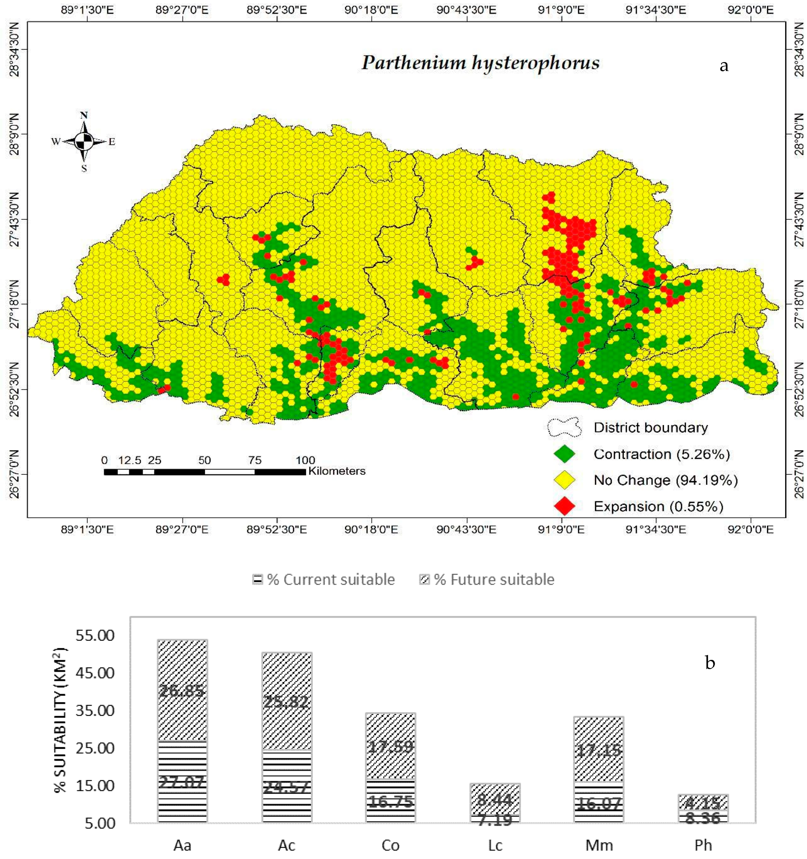
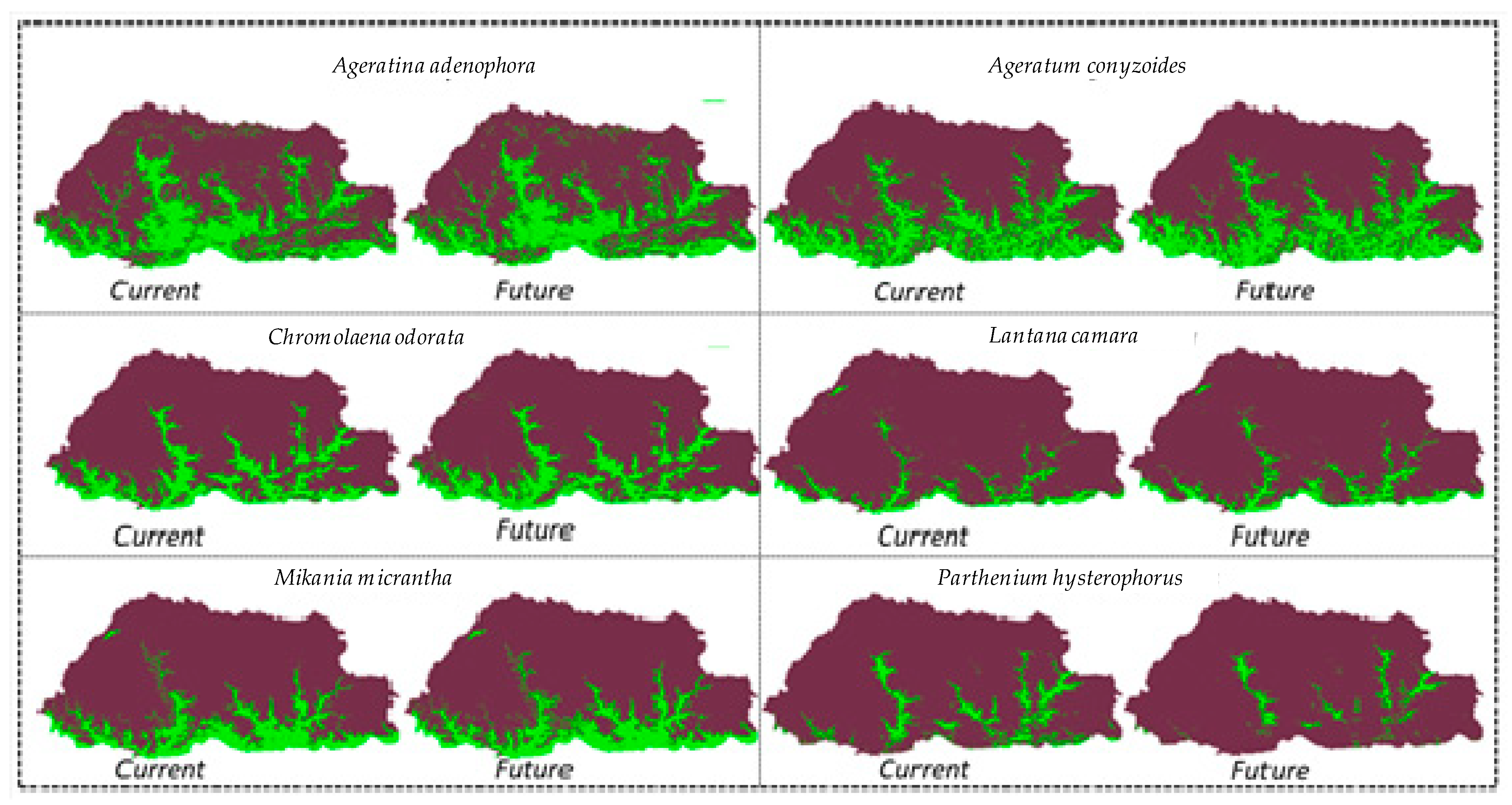
3.2. Spatial Change Analysis

For P. hysterophorus, the area of expansion (0.55%) was much less than its area of contraction (5.26%) under the future climatic condition (Figure 1a) when compared with the other species (Figure S2). In terms of absolute change, the area of invasion increased in the case of A. conyzoides (Ac), C. odorata (Co), L. camara (Lc), and M. micrantha (Mm), while it decreased for A. adenophora (Aa = 27.07% to 26.85%) and P. hysterophorus (Ph = 8.36% to 4.15%) (Figure 1b). Ageratina adenophora and A. conyzoides appeared to be the most gregarious species (Figure S2), while P. hysterophorus appeared to be the most intolerant to changes in climatic conditions. According to Wan et al. [70], A. adenophora exhibits morphological and structural plasticity to adapt to the environment in invaded areas through genetic diversification. Furthermore, He et al. [71] reported a positive correlation between the stomatal density and altitude, thus attributing A. adenophora’s adaptability to higher temperature and lower humidity in high altitude areas. Similar to the report by Lamsal et al. [21], the spread of P. hysterophorus decreased in this study, which could be because this species thrives mostly in agroecosystems and grasslands [22], and in Bhutan, the land cover is dominated by forests, as high as 71%. Parthenium hysterophorus is also very sensitive to photoperiodic fluxes and temperature changes [72], which are very common in Bhutan due to its high topographical variability [73,74]. In contrast, A. adenophora, A. conyzoides, C. odorata, L. camara, and M. micrantha are characterized as forest understory invaders with a high dispersal mobility [22].

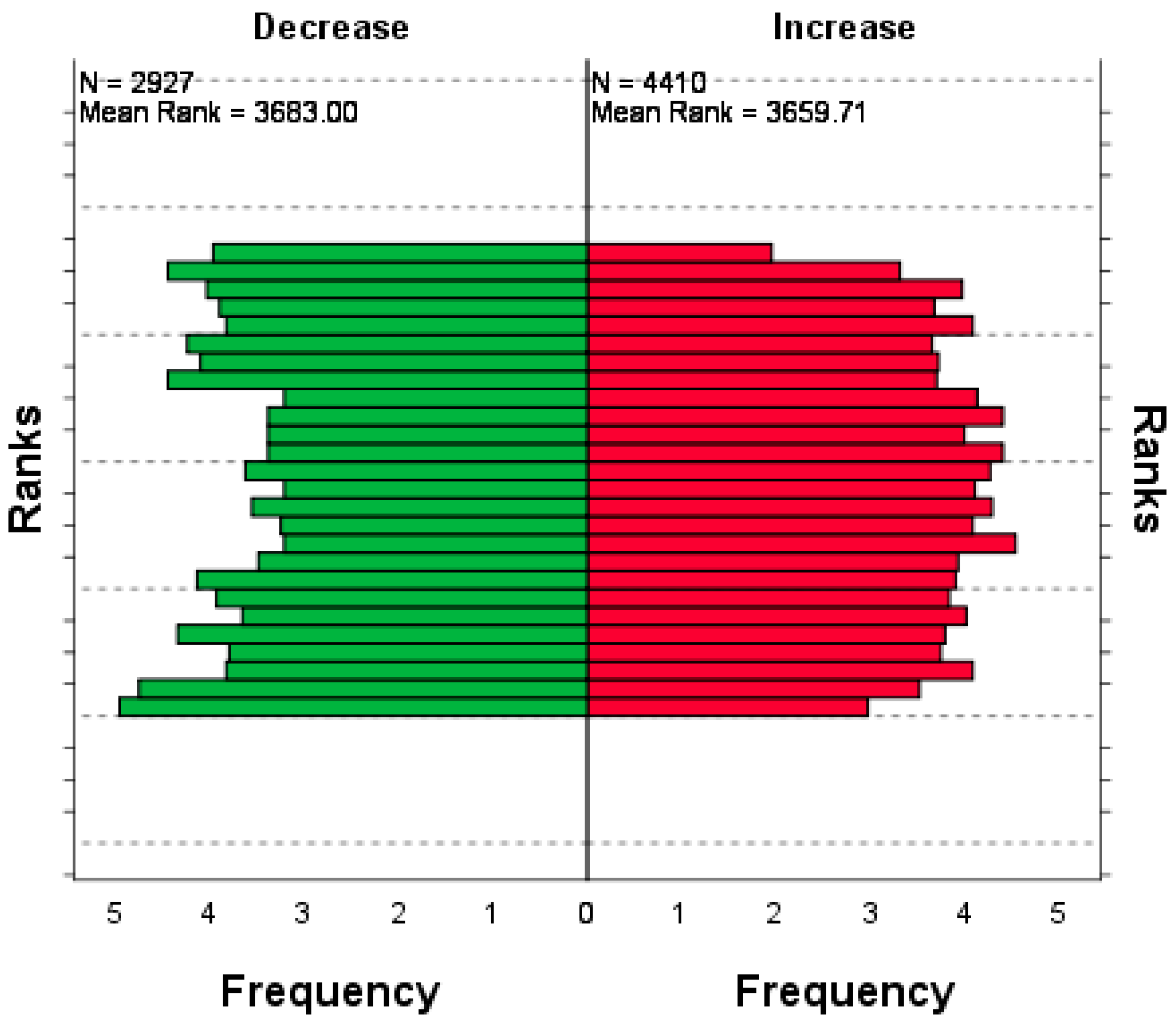
3.3. Testing the Statistical Significance of Changes

The model predictions of decrease and increase in areas of invasion in the future climatic scenario were tested using Wilcoxon Signed-Ranks Tests. The decrease in area (4.15%) was significant for P. hysterophorus (Z = 2.766, p = 0.006), and the decrease in area (26.85%) was non-significant for A. adenophora (Z = 0.371, p = 0.711). The increase in area (17.59%) was significant for C. odorata (Z = 2.785, p = 0.005), while the increase in areas (25.82%, 8.44%, and 17.15%) were non-significant for A. conyzoides (Z = 1.063, p = 0.288), L. camara (Z = 0.642, p = 0.521), and M. micrantha (Z = 0.751, p = 0.453), respectively. Therefore, P. hysterophorus can be characterized as intolerant, and C. odorata is adaptable to changing climate (see the rate of change in Figure S2 and standard ellipse in Figure S3). However, P. hysterophorus was predicted to be highly invasive under future climatic scenarios in the landscape of Nepal [22]. This difference could be attributed to the fact that Bhutan is predominantly covered by forests [75,76], which act as natural barriers to the mobility of the species. Parthenium hysterophorus seeds are mainly dispersed by vehicular movements and are found in disturbed areas such as agricultural lands, roadsides, river banks, and wastelands [22].

A Mann–Whitney U test showed that there was no significant difference (U = 6413057, p = 0.645) between the increase in area of predicted invasion compared to the decrease in area of predicted invasion when all species were combined across the study area (Figure 2). This underscores the fact that Bhutan has primarily intact forests, of which 52% are totally protected as national parks, wildlife sanctuaries, and biological corridors [76]. Furthermore, the species in question more or less prefer habitats along roadsides, degraded lands, pastures, and agricultural fields.

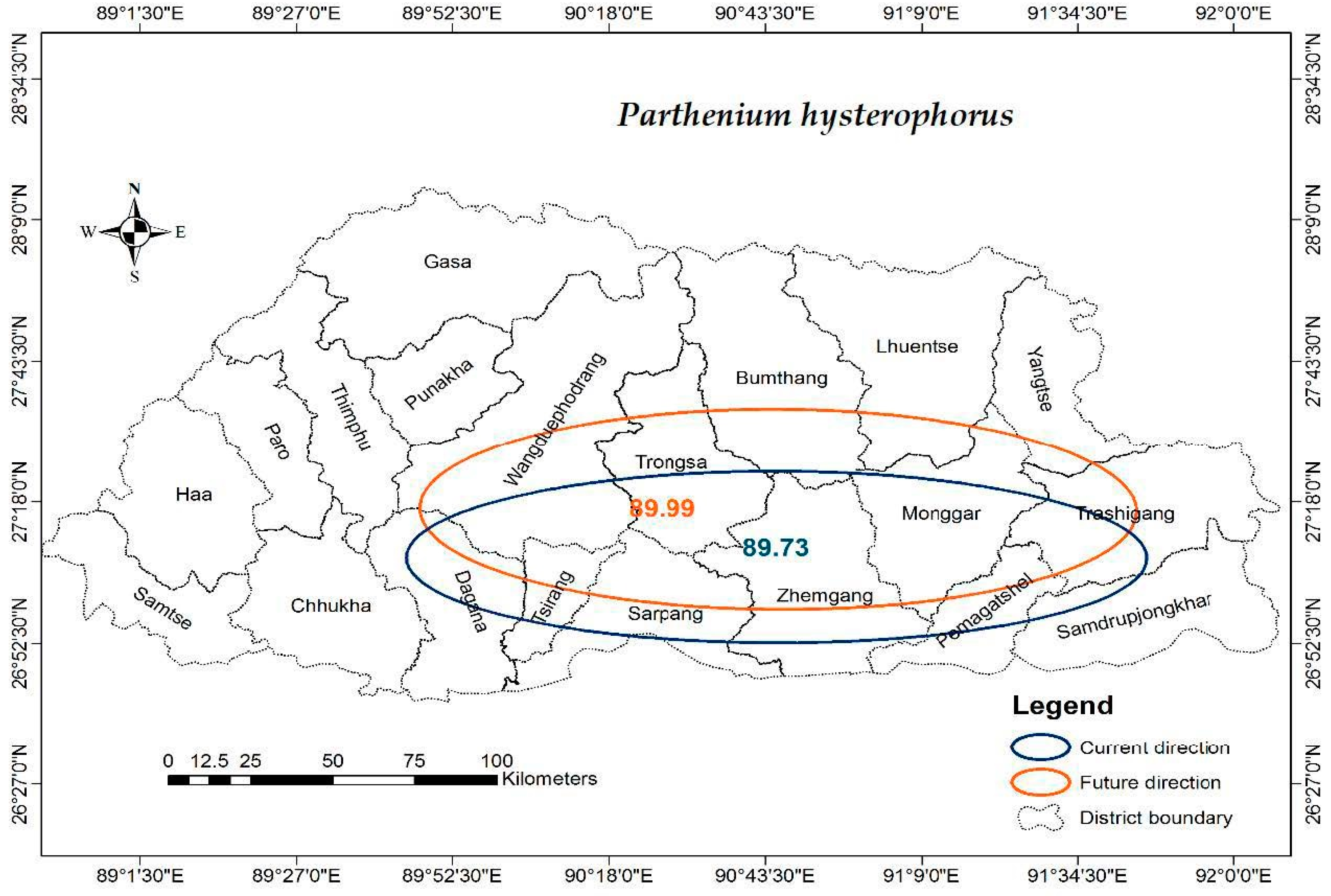
3.4. Cardinal Directions of Distributions

The directional distribution in the current climatic scenario (blue ellipse) followed angles of rotation from 87.06° to 89.73° northeast and 92.22° to 92.88° southeast, while in the future (orange ellipse) it followed from 78.74° to 89.99° northeast and 90.41° to 93.04° southeast (see Supplementary Material Figure S3). The directional distribution of A. conyzoides became almost a perfect circle in the future climatic scenario, which according to the algorithm of standard deviational ellipse represents a dispersion in distribution. There was also a notable northward shift in the distribution of P. hysterophorus from the current to the future scenario as seen in Figure 3. Such observations are in accordance with the findings that climate change can disrupt species distributional patterns [64,77,78,79,80] by the process of colonization and removal of local species through competition.

3.5. Limitations and Caveats of the Model

As in the case of any correlative modeling, Maxent modeling has its limitations. Maxent assumes that the sampling effort is uniform across the entire area of interest and that the prevalence of occurrence is 50% or more, while in practice, the models are developed from the occurrence records of accessible areas, thus tending toward a spatial bias [61,81]. Furthermore, the interpretation of the results should be treated from an inductive rather than deductive perspective, which means that such models are to build rather than test the hypothesis. As such, models demand several iterations to account for the effects of sample sizes [82,83], the spatial scales of the area of interest, the spatial resolutions of the predictors [84], the selection of biologically meaningful environmental predictors [85], and different filtering levels of autocorrelations of occurrence records [86] to enhance model fidelity and consistency.

To circumvent the limitations above, this study undertook measures such as planning the sampling design by considering the population viability within the plots and reduction of spatial autocorrelation. Furthermore, the multicollinearity of predictor variables was removed and their biological usefulness considered. This study, therefore, remains fairly robust, relative to those that have resorted to using secondary data from museums, herbaria, or online databases (e.g., GBIF) that have been collected on an ad hoc basis.

4. Conclusions

Our model predictions conformed to the established theory that invasion is facilitated by climate change since areas of predicted invasion increased during future climate scenarios. One notable indication of this study was that the projection of current to future predictions could lead to weaker power of the Maxent model (partial AUC values decreased from current to future climate scenarios). This occurs when the correlation between the response and predictors may only be adequate over a narrow range of spatial and temporal scales. Among the six species, C. odorata could become more prevalent over time, while P. hysterophorus may be very sensitive to climate change, as indicated by its northward shift with a decrease in extent. Despite expansion in areas under the future climatic condition, most species appear to limit their invasion to the southern region (S2: 26°52′30″ N to 27°18′0″ N) of the country. Lantana camara turned out to be the most stable species to change in climatic conditions (No change = 97.49%), in contrast to P. hysterophorus, which was the most unstable species to climate change (No change = 94.19%). Statistical non-significance of the Mann–Whitney U test reinforced that overall, there is no significant impact of climatic change on invasion. Such a unique result could be due to the country’s strong policies on environmental protection such as the delimitation of protected areas, banning slash and burn agriculture practices, and the plant quarantine act. However, the ruggedness of the mountain terrain cannot be overruled as a limiting factor. This study not only points out which species are more likely to respond positively and negatively to changes in climatic conditions, but also provides the directions of potential spread in the geographical space. This approach can serve as the basis for strategic control (e.g., plant quarantine policy implementation using transborder screening) of the species in question as well as further studies into these species such as detection surveys.

References

1. Ihlow, F.; Courant, J.; Secondi, J.; Herrel, A.; Rebelo, R.; Measey, G.J.; Lillo, F.; De Villiers, F.A.; Vogt, S.; De Busschere, C.; et al. Impacts of climate change on the global invasion potential of the African clawed frog Xenopus laevis. PLoS ONE 2016, 11. [Google Scholar] [CrossRef] [PubMed]
2. Lourenco-de-Moraes, R.; Lansac-Toha, F.M.; Schwind, L.T.F.; Arrieira, R.L.; Rosa, R.R.; Terribile, L.C.; Lemess, P.; Rangel, T.F.; Diniz, J.A.F.; Bastosz, R.P.; et al. Climate change will decrease the range size of snake species under negligible protection in the Brazilian Atlantic forest hotspot. Sci. Rep. 2019, 9. [Google Scholar] [CrossRef] [PubMed]
3. Mohapatra, J.; Singh, C.P.; Hamid, M.; Verma, A.; Semwal, S.C.; Gajmer, B.; Khuroo, A.A.; Kumar, A.; Nautiyal, M.C.; Sharma, N.; et al. Modelling Betula utilis distribution in response to climate-warming scenarios in Hindu-Kush Himalaya using random forest. Biodivers. Conserv. 2019, 28, 2295–2317. [Google Scholar] [CrossRef]
4. Priyanka, N.; Joshi, P.K. Effects of climate change on invasion potential distribution of Lantana camara. J. Earth Sci. Clim. Chang. 2013, 4, 164. [Google Scholar] [CrossRef]
5. Rathore, P.; Roy, A.; Karnatak, H. Assessing the vulnerability of Oak (Quercus) forest ecosystems under projected climate and land use land cover changes in Western Himalaya. Biodivers. Conserv. 2019, 28, 2275–2294. [Google Scholar] [CrossRef]
6. Ruaro, R.; Conceicao, E.O.; Silva, J.C.; Cafofo, E.G.; Angulo-Valencia, M.A.; Mantovano, T.; Pineda, A.; de Paula, A.C.M.; Zanco, B.F.; Capparros, E.M.; et al. Climate change will decrease the range of a keystone fish species in La Plata river basin, South America. Hydrobiologia 2019, 836, 1–19. [Google Scholar] [CrossRef]
7. Saupe, E.E.; Myers, C.E.; Peterson, A.T.; Soberon, J.; Singarayer, J.; Valdes, P.; Qiao, H.J. Non-random latitudinal gradients in range size and niche breadth predicted by spatial patterns of climate. Glob. Ecol. Biogeogr. 2019, 28, 928–942. [Google Scholar] [CrossRef]
8. Wang, C.J.; Wan, J.Z.; Zhang, Z.X. Will Global climate change facilitate plant invasions in conservation areas? Pak. J. Bot. 2019, 51, 1395–1403. [Google Scholar] [CrossRef]
9. Bugmann, H.; Gurung, A.B.; Ewert, F.; Haeberli, W.; Guisan, A.; Fagre, D.; Kaab, A.; Participants, G. Modeling the biophysical impacts of global change in mountain biosphere reserves. Mt. Res. Dev. 2007, 27, 66–77. [Google Scholar] [CrossRef]
10. De la Hoz, C.F.; Ramos, E.; Puente, A.; Juanes, J.A. Climate change induced range shifts in seaweeds distributions in Europe. Mar. Environ. Res. 2019, 148, 1–11. [Google Scholar] [CrossRef]
11. Intergovernmental Panel on Climate Change (IPCC). Global Warming of 1.5 C; Report; IPCC: Geneva, Switzerland, 2018. [Google Scholar]
12. Geng, Y.P.; Pan, X.Y.; Xu, C.Y.; Zhang, W.J.; Li, B.; Chen, J.K. Phenotypic plasticity of invasive Alternanthera philoxeroides in relation to different water availability, compared to its native congener. Acta Oecol. 2006, 30, 380–385. [Google Scholar] [CrossRef]
13. Keser, L.H.; Dawson, W.; Song, Y.B.; Yu, F.H.; Fischer, M.; Dong, M.; van Kleunen, M. Invasive clonal plant species have a greater root-foraging plasticity than non-invasive ones. Oecologia 2014, 174, 1055–1064. [Google Scholar] [CrossRef] [PubMed]
14. Liu, Y.; Oduor, A.M.; Zhang, Z.; Manea, A.; Tooth, I.M.; Leishman, M.R.; Xu, X.; Van Kleunen, M. Do invasive alien plants benefit more from global environmental change than native plants? Glob. Chang. Biol. 2017, 23, 3363–3370. [Google Scholar] [CrossRef] [PubMed] [Green Version]
15. Chown, S.L.; Hodgins, K.A.; Griffin, P.C.; Oakeshott, J.G.; Byrne, M.; Hoffmann, A.A. Biological invasions, climate change and genomics. Evol. Appl. 2015, 8, 23–46. [Google Scholar] [CrossRef] [PubMed]
16. Bradley, B.A.; Wilcove, D.S.; Oppenheimer, M. Climate change increases risk of plant invasion in the Eastern United States. Biol. Invasions 2010, 12, 1855–1872. [Google Scholar] [CrossRef]
17. Keller, S.; Taylor, D. Genomic admixture increases fitness during a biological invasion. J. Evol. Biol. 2010, 23, 1720–1731. [Google Scholar] [CrossRef] [PubMed]
18. Tecco, P.A.; Pais-Bosch, A.I.; Funes, G.; Marcora, P.I.; Zeballos, S.R.; Cabido, M.; Urcelay, C. Mountain invasions on the way: Are there climatic constraints for the expansion of alien woody species along an elevation gradient in Argentina? J. Plant Ecol. 2015, 9, 380–392. [Google Scholar] [CrossRef]
19. Eckholm, E.P. The deterioration of mountain environments. Science 1975, 189, 764–770. [Google Scholar] [CrossRef]
20. McDougall, K.L.; Khuroo, A.A.; Loope, L.L.; Parks, C.G.; Pauchard, A.; Reshi, Z.A.; Rushworth, I.; Kueffer, C. Plant Invasions in mountains: Global lessons for better management. Mt. Res. Dev. 2011, 31, 380–387. [Google Scholar] [CrossRef]
21. Lamsal, P.; Kumar, L.; Aryal, A.; Atreya, K. Invasive alien plant species dynamics in the Himalayan region under climate change. Ambio 2018, 47, 697–710. [Google Scholar] [CrossRef]
22. Shrestha, U.B.; Sharma, K.P.; Devkota, A.; Siwakoti, M.; Shrestha, B.B. Potential impact of climate change on the distribution of six invasive alien plants in Nepal. Ecol. Indic. 2018, 95, 99–107. [Google Scholar] [CrossRef]
23. Thapa, S.; Chitale, V.; Rijal, S.J.; Bisht, N.; Shrestha, B.B. Understanding the dynamics in distribution of invasive alien plant species under predicted climate change in Western Himalaya. PLoS ONE 2018, 13, e0195752. [Google Scholar] [CrossRef] [PubMed]
24. Hoy, A.; Katel, O. Status of Climate Change and Implications to Ecology and Community Livelihoods in the Bhutan Himalaya. In Environmental Change in the Himalayan Region; Springer: Cham, Switzerland, 2019; pp. 23–45. [Google Scholar]
25. Penuelas, J.; Boada, M. A global change-induced biome shift in the Montseny mountains (NE Spain). Glob. Chang. Biol. 2003, 9, 131–140. [Google Scholar] [CrossRef] [Green Version]
26. Suberi, B.; Tiwari, K.R.; Gurung, D.B.; Bajracharya, R.M.; Sitaula, B.K. People’s perception of climate change impacts and their adaptation practices in Khotokha valley, Wangdue, Bhutan. Indian J. Tradit. Knowl. 2018, 17, 97–105. [Google Scholar]
27. McDougall, K.L.; Alexander, J.M.; Haider, S.; Pauchard, A.; Walsh, N.G.; Kueffer, C. Alien flora of mountains: Global comparisons for the development of local preventive measures against plant invasions. Divers. Distrib. 2011, 17, 103–111. [Google Scholar] [CrossRef]
28. Seldon, P. First ever Bhutan Climate Report Predicts a Hotter and Wetter Bhutan. The Bhutanese. Available online: https://thebhutanese.bt/first-ever-bhutan-climate-report-predicts-a-hotter-and-wetter-bhutan/ (accessed on 3 March 2019).
29. Fort, M. Impact of climate change on mountain environment dynamics. An introduction. J. Alp. Res. 2015. [Google Scholar] [CrossRef]
30. Beniston, M. Mountain Environments in Changing Climates; Beniston, M., Ed.; Routledge: London, UK; New York, NY, USA, 2002. [Google Scholar]
31. International Centre for Integrated Mountain Development (Nepal) (ICIMOD). Climate Change Impacts and Vulnerabilities in the Eastern Himalayas; ICIMOD: Lalitpur, Nepal, 2009. [Google Scholar]
32. Malanson, G.P.; Fagre, D.B. Spatial contexts for temporal variability in alpine vegetation under ongoing climate change. Plant Ecol. 2013, 214, 1309–1319. [Google Scholar] [CrossRef]
33. Williamson, M.H.; Fitter, A. The characters of successful invaders. Biol. Conserv. 1996, 78, 163–170. [Google Scholar] [CrossRef]
34. Rejmanek, M.; Richardson, D.M. What attributes make some plant species more invasive? Ecology 1996, 77, 1655–1661. [Google Scholar] [CrossRef]
35. Sutherland, S. What makes a weed a weed: Life history traits of native and exotic plants in the USA. Oecologia 2004, 141, 24–39. [Google Scholar] [CrossRef]
36. Devin, S.; Beisel, J.N. Biological and ecological characteristics of invasive species: A gammarid study. Biol. Invasions 2007, 9, 13–24. [Google Scholar] [CrossRef]
37. Maron, J.L.; Vilà, M.; Bommarco, R.; Elmendorf, S.; Beardsley, P. Rapid evolution of an invasive plant. Ecol. Monogr. 2004, 74, 261–280. [Google Scholar] [CrossRef]
38. Higgins, S.I.; Richardson, D.M. Invasive plants have broader physiological niches. Proc. Natl. Acad. Sci. USA 2014, 111, 10610–10614. [Google Scholar] [CrossRef] [PubMed] [Green Version]
39. Funk, J.L. The physiology of invasive plants in low-resource environments. Conserv. Physiol. 2013, 1. [Google Scholar] [CrossRef] [PubMed]
40. Royal Government of Bhutan. Forest and Nature Conservation Rules and Regulations of Bhutan; Department of Forest and Park Services: Thimphu, Butan, 2017.
41. Chhetri, P.B.; Tenzin, K. Bhutan: The State of the World’s Forest Genetic Resources—FAO; RNR Research and Development Centre: Yusipang, Bhutan, 2012.
42. National Biodiversity Centre (NBC). Bhutan-Biodiversity Action Plan 2009—UNDP in Bhutan; NBC: Thimphu, Bhutan, 2009. [Google Scholar]
43. Grierson, A.J.C.; Long, D.G. Flora of Bhutan. NORDIC J. Bot. 2001, 2, 456. [Google Scholar] [CrossRef]
44. Parker, C. Weeds of Bhutan; National Palnt Protection Centre: Thimphu, Bhutan, 1992.
45. Bhutan Biodiversity Portal. Available online: https://biodiversity.bt/ (accessed on 1 August 2019).
46. Pallewatta, N.; Reaser, J.; Gutierrez, A. Invasive Alien Species in South-Southeast Asia: National Reports and Directory of Resources; Global Invasive Species Programme: Cape Town, South Africa, 2003. [Google Scholar]
47. Tallis, H.; Kareiva, P.; Marvier, M.; Chang, A. An ecosystem services framework to support both practical conservation and economic development. Proc. Natl. Acad. Sci. USA 2008, 105, 9457–9464. [Google Scholar] [CrossRef] [PubMed] [Green Version]
48. Peterson, A.T.; Navarro-Sigüenza, A.G.; Martínez-Meyer, E.; Cuervo-Robayo, A.P.; Berlanga, H.; Soberón, J. Twentieth century turnover of Mexican endemic avifaunas: Landscape change versus climate drivers. Sci. Adv. 2015, 1, e1400071. [Google Scholar] [CrossRef] [PubMed]
49. Choudhury, M.R.; Deb, P.; Singha, H.; Chakdar, B.; Medhi, M. Predicting the probable distribution and threat of invasive Mimosa diplotricha Suavalle and Mikania micrantha Kunth in a protected tropical grassland. Ecol. Eng. 2016, 97, 23–31. [Google Scholar] [CrossRef]
50. Keith, D.A.; Akcakaya, H.R.; Thuiller, W.; Midgley, G.F.; Pearson, R.G.; Phillips, S.J.; Regan, H.M.; Araujo, M.B.; Rebelo, T.G. Predicting extinction risks under climate change: Coupling stochastic population models with dynamic bioclimatic habitat models. Biol. Lett. 2008, 4, 560–563. [Google Scholar] [CrossRef] [PubMed]
51. López-Darias, M.; Lobo, J.M.; Gouat, P. Predicting potential distributions of invasive species: The exotic Barbary ground squirrel in the Canarian archipelago and the west Mediterranean region. Biol. Invasions 2007, 10, 1027–1040. [Google Scholar] [CrossRef]
52. Pearson, R.G.; Dawson, T.P. Predicting the impacts of climate change on the distribution of species: Are bioclimate envelope models useful? Glob. Ecol. Biogeogr. 2003, 12, 361–371. [Google Scholar] [CrossRef]
53. Stiels, D.; Schidelko, K.; Engler, J.O.; van den Elzen, R.; Rödder, D. Predicting the potential distribution of the invasive Common Waxbill Estrilda astrild (Passeriformes: Estrildidae). J. Ornithol. 2011, 152, 769–780. [Google Scholar] [CrossRef]
54. Elith, J.; Leathwick, J.R. Species distribution models: Ecological explanation and prediction across space and time. Annu. Rev. Ecol. Evol. Syst. 2009, 40, 677–697. [Google Scholar] [CrossRef]
55. Merow, C.; Allen, J.M.; Aiello-Lammens, M.; Silander, J.A. Improving niche and range estimates with Maxent and point process models by integrating spatially explicit information. Glob. Ecol. Biogeogr. 2016, 25, 1022–1036. [Google Scholar] [CrossRef]
56. Ray, D.; Behera, M.D.; Jacob, J. Evaluating Ecological Niche Models: A Comparison Between Maxent and GARP for Predicting Distribution of Hevea brasiliensis in India. Proc. Indian Natl. Sci. Acad. Part B Biol. Sci. 2018, 88, 1337–1343. [Google Scholar] [CrossRef]
57. Zhang, L.; Liu, S.; Sun, P.; Wang, T.; Wang, G.; Zhang, X.; Wang, L. Consensus forecasting of species distributions: The effects of niche model performance and niche properties. PLoS ONE 2015, 10, e0120056. [Google Scholar] [CrossRef] [PubMed]
58. Peterson, A.T.; Papeş, M.; Soberón, J. Rethinking receiver operating characteristic analysis applications in ecological niche modeling. Ecol. Model. 2008, 213, 63–72. [Google Scholar] [CrossRef]
59. Pearson, R.G.; Raxworthy, C.J.; Nakamura, M.; Townsend Peterson, A. Predicting species distributions from small numbers of occurrence records: A test case using cryptic geckos in Madagascar. J. Biogeogr. 2007, 34, 102–117. [Google Scholar] [CrossRef]
60. Ashraf, U.; Peterson, A.T.; Chaudhry, M.N.; Ashraf, I.; Saqib, Z.; Ahmad, S.R.; Ali, H. Ecological niche model comparison under different climate scenarios: A case study of Olea spp. in Asia. Ecosphere 2017, 8, e01825. [Google Scholar] [CrossRef]
61. Kramer-Schadt, S.; Niedballa, J.; Pilgrim, J.D.; Schröder, B.; Lindenborn, J.; Reinfelder, V.; Stillfried, M.; Heckmann, I.; Scharf, A.K.; Augeri, D.M. The importance of correcting for sampling bias in MaxEnt species distribution models. Divers. Distrib. 2013, 19, 1366–1379. [Google Scholar] [CrossRef]
62. Phillips, S.J.; Anderson, R.P.; Schapire, R.E. Maximum entropy modeling of species geographic distributions. Ecol. Model. 2006, 190, 231–259. [Google Scholar] [CrossRef] [Green Version]
63. Ohsawa, M.E. Life Zone Ecology of the Bhutan Himalaya; Laboratory of Ecology, Chiba University: Chiba, Japan, 1987. [Google Scholar]
64. Pearson, R.G. Species’ Distribution Modeling for Conservation Educators and Practitioners. Lessons Conserv. 2008, 3, 54–89. [Google Scholar]
65. Brown, J.L. SDMtoolbox: A python-based GIS toolkit for landscape genetic, biogeographic and species distribution model analyses. Methods Ecol. Evol. 2014, 5, 694–700. [Google Scholar] [CrossRef]
66. Hijmans, R.; Cameron, S.; Parra, J.; Jones, P.; Jarvis, A.; Richardson, K. WorldClim, version 1.3; University of California: Berkeley, CA, USA, 2005. [Google Scholar]
67. Phillips, S.J.; Dudik, M.; Schapire, R. MaxEnt, Version 3.3. 3k; AT & T Labs-Research, Princeton University: Princeton, NJ, USA, 2012. [Google Scholar]
68. Environmental Systems Research Institute (ESRI). ArcGIS Desktop: Release 10.1. Available online: https://www.esri.com/news/arcnews/spring12articles/introducing-arcgis-101.html (accessed on 26 January 2015).
69. Pitt, J.P.W.; Kriticos, D.J.; Dodd, M.B. Temporal limits to simulating the future spread pattern of invasive species: Buddleja davidii in Europe and New Zealand. Ecol. Model. 2011, 222, 1880–1887. [Google Scholar] [CrossRef]
70. Wan, F.; Liu, W.; Guo, J.; Qiang, S.; Li, B.; Wang, J.; Yang, G.; Niu, H.; Gui, F.; Huang, W. Invasive mechanism and control strategy of Ageratina adenophora (Sprengel). Sci. China Life Sci. 2010, 53, 1291–1298. [Google Scholar] [CrossRef] [PubMed]
71. He, J.Y.; Qiang, S.; Song, X.L.; Jin, H.Y. Comparison of the stem and leaf morphological structures of 18 communities of the foreign plant Eupatorium adenophorum. Acta Bot. Sin. 2005, 25, 1089. [Google Scholar]
72. Kaur, A.; Batish, D.R.; Kaur, S.; Singh, H.P.; Kohli, R.K. Phenological behaviour of Parthenium hysterophorus in response to climatic variations according to the extended BBCH scale. Ann. Appl. Biol. 2017, 171, 316–326. [Google Scholar] [CrossRef]
73. Ura, K.; Kinga, S. Bhutan—Sustainable Development through Good Governance; World Bank: Washington, DC, USA, 2004. [Google Scholar]
74. Regmi, B.; Pandit, A.; Pradhan, B.; Kovats, S.; Lama, P. Capacity Strengthening in the Least Developed Countries (LDCs) for Adaptation to Climate Change (CLACC), Climate Change and Health in Nepal. Available online: https://pubs.iied.org/pdfs/G02664.pdf? (accessed on 1 May 2019).
75. Penjore, D.; Rapten, P. Trends of forestry policy concerning local participation in Bhutan. Forest 2004, 25, 21–27. [Google Scholar]
76. Department of Forests and Park Services. Forest Facts and Figures. Available online: http://www.dofps.gov.bt/wp-content/uploads/2017/07/ForestBookletFinal.pdf (accessed on 18 May 2019).
77. Franklin, J. Moving beyond static species distribution models in support of conservation biogeography. Divers. Distrib. 2010, 16, 321–330. [Google Scholar] [CrossRef]
78. Paini, D.R.; Sheppard, A.W.; Cook, D.C.; De Barro, P.J.; Worner, S.P.; Thomas, M.B. Global threat to agriculture from invasive species. Proc. Natl. Acad. Sci. USA 2016, 113, 7575–7579. [Google Scholar] [CrossRef] [Green Version]
79. Peterson, A.T.; Papeş, M.; Soberón, J. Mechanistic and correlative models of ecological niches. Eur. J. Ecol. 2015, 1, 28–38. [Google Scholar] [CrossRef]
80. Franklin, J. Mapping Species Distribution; Cambridge University Press: New York, NY, USA, 2009. [Google Scholar]
81. Jarnevich, C.S.; Stohlgren, T.J.; Kumar, S.; Morisette, J.T.; Holcombe, T.R. Caveats for correlative species distribution modeling. Ecol. Inform. 2015, 29, 6–15. [Google Scholar] [CrossRef]
82. Hernandez, P.A.; Graham, C.H.; Master, L.L.; Albert, D.L. The effect of sample size and species characteristics on performance of different species distribution modeling methods. Ecography 2006, 29, 773–785. [Google Scholar] [CrossRef]
83. Wisz, M.S.; Hijmans, R.J.; Li, J.; Peterson, A.T.; Graham, C.H.; Guisan, A. NCEAS Predicting Species Distributions Working Group. Effects of sample size on the performance of species distribution models. Divers. Distrib. 2008, 14, 763–773. [Google Scholar] [CrossRef]
84. Guisan, A.; Graham, C.H.; Elith, J.; Huettmann, F.; NCEAS Species Distribution Modelling Group. Sensitivity of predictive species distribution models to change in grain size. Divers. Distrib. 2007, 13, 332–340. [Google Scholar] [CrossRef]
85. Naimi, B.; Skidmore, A.K.; Groen, T.A.; Hamm, N.A.S. Spatial autocorrelation in predictors reduces the impact of positional uncertainty in occurrence data on species distribution modeling. J. Biogeogr. 2011, 38, 1497–1509. [Google Scholar] [CrossRef]
86. Boria, R.A.; Olson, L.E.; Goodman, S.M.; Anderson, R.P. Spatial filtering to reduce sampling bias can improve the performance of ecological niche models. Ecol. Model. 2014, 275, 73–77. [Google Scholar] [CrossRef]
Figure 1. (a) Hexagonally binned-map illustrating the rate of change in areas of distribution of P. hysterophorus across the study area. Contraction = decrease in rate, Expansion = increase in rate, and No Change = neither a decrease nor increase in rate with respect to the future climate scenario. (b) Percent of predicted invasion by areas in the current and future climatic scenarios. Aa = A. adenophora, Ac = A. conyzoides, Co = C. odorata, Lc = L. camara, Mm = M. micrantha, and Ph = P. hysterophorus.
Agronomy 09 00442 g001
Figure 2. Showing the differences in the mean ranks of increase and decrease in areas of invasion between the two climate scenarios.
Agronomy 09 00442 g002
Figure 3. Predicted directional distributions of P. hysterophorus in the two climatic conditions.
Agronomy 09 00442 g003