AquaCropR: Crop Growth Model for R

Abstract
:1. Introduction
2. AquaCropR Overview
2.1. Open Source
2.2. eXtensible Markup Language (XML)
2.3. AquaCropR—New Functions
2.3.1. Evapotranspiration (ETo)
2.3.2. Solar Radiation
2.3.3. Sowing Date Estimation
2.3.4. Optimisation Module
3. Installation and Running AquaCropR
3.1. Installation
- Clone the AquaCrop repository
- Run R
- Install the devtools package (if not available already)install.packages(“devtools”)
- Load the devtools package.library(devtools)
- Set working directory to AquaCrop’s locationsetwd(‘your location/AquaCropR’)
- Set working directory a level above AquaCropRsetwd(‘..’)
- Install AquaCropRInstall(‘AquaCropR’)
- Use the following command to test AquaCropR’s installation?? AquaCropR
3.2. Running a Simulation
- Clone the AquaCropExamples repositoryCheck that the ‘input_wheat_tunis_s1′ folder was pulled from the ‘AquaExamples’ repository.
- Load R
- Load AquaCropR packagelibrary(AquaCropR)
- Load crop simulation parameter files.FileLocation = ReadFileLocations(pathname/input_wheat_tunis_cropot/filesetup.xml’)Where pathname correspond to the location folder where the ‘AquaExamples’ repo was installed (e.g., ‘repo/AquaExamples’)
- Initialise the model using crop and simulation parametersInitialiseStruct <- Initialise(FileLocation)
- Run the simulation and view the results dataset. Check the AquaCropR tutorial for definition of the variables returned in the Simulation Results dataset.Outputs <- PerformSimulation(InitialiseStruct)
4. Testing and Evaluation
4.1. Maize Exercise
4.2. Wheat Exercises
4.2.1. Wheat Scenario 1: Default Soil
4.2.2. Wheat Scenario 2: A Typical Local Soil
4.2.3. Wheat Scenario 3: A Late-Maturing Wheat Variety
- Time from sowing to emergence (GDD) = 289
- Time from sowing to flowering (GDD) = 1073
- Time from sowing to senescence (GDD) = 2835
- Time from sowing to physiological maturity (GDD) = 3390
- Duration of flowering (GDD) = 264
- Planting density (plants m−2) = 350
- Maximum canopy cover (%) = 90
4.2.4. Wheat Scenario 4: Applying an Irrigation Schedule
4.3. Results
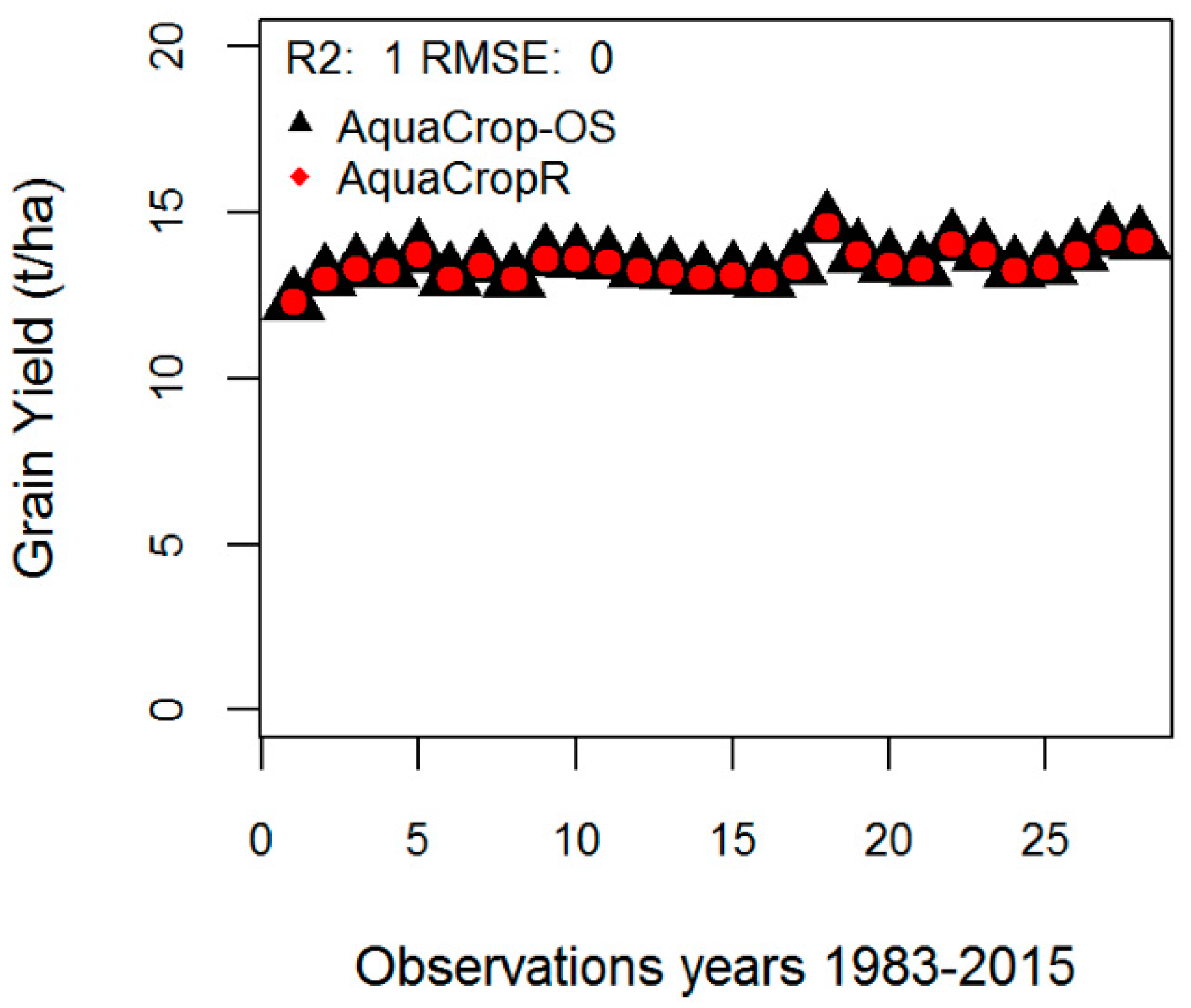
4.3.1. Maize
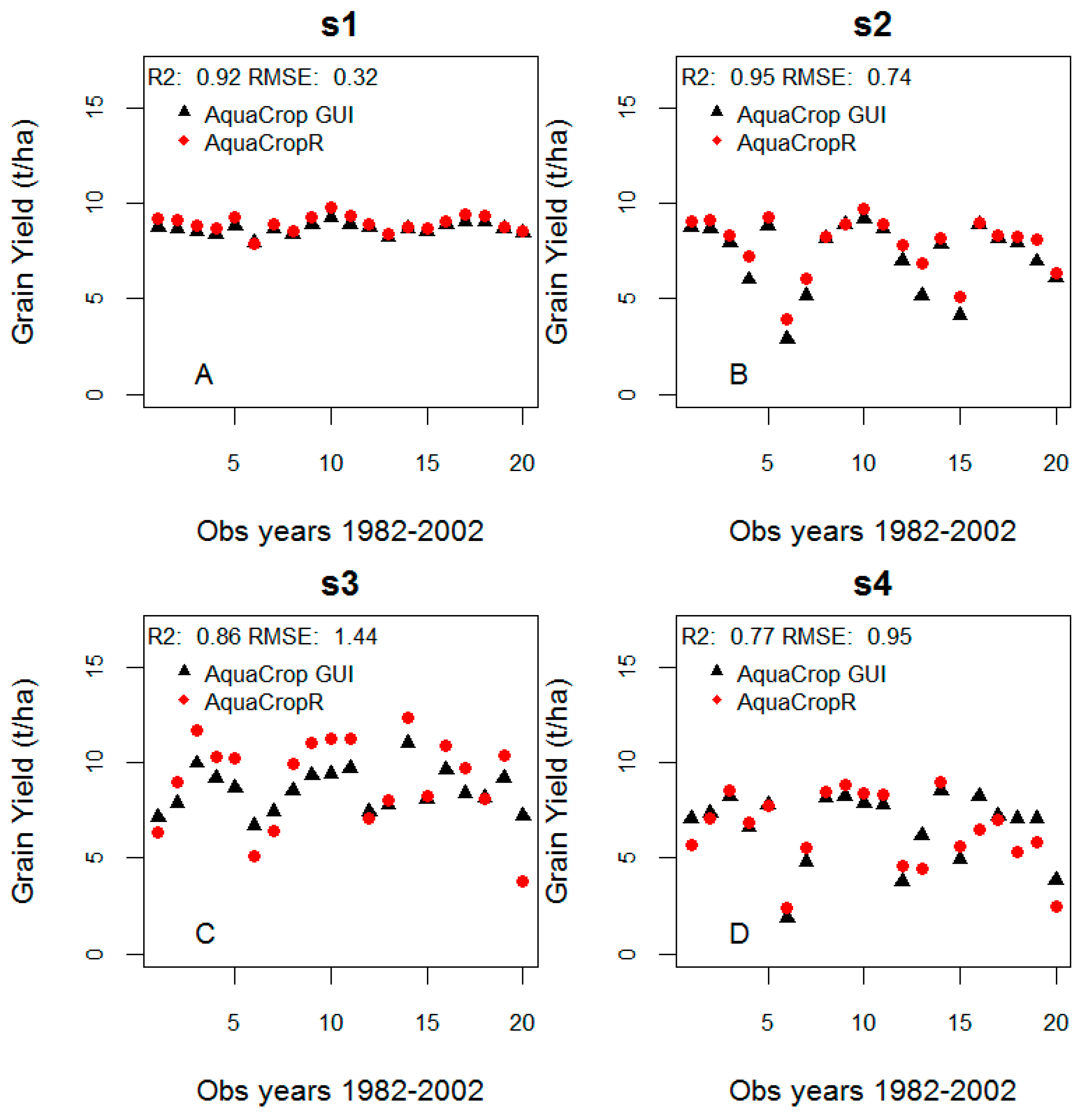
4.3.2. Wheat
5. Summary
Author Contributions
Funding
Acknowledgments
Conflicts of Interest
References
- Porfirio, L.L.; Newth, D.; Finnigan, J.J.; Cai, Y. Economic shifts in agricultural production and trade due to climate change. Palgrave Commun. 2018, 4, 111. [Google Scholar] [CrossRef]
- Chenu, K.; Porter, J.R.; Martre, P.; Basso, B.; Chapman, S.C.; Ewert, F.; Bindi, M.; Asseng, S. Contribution of crop models to adaptation in wheat. Trends Plant Sci. 2017, 22, 472–490. [Google Scholar] [CrossRef] [PubMed]
- Lipper, L.; Thornton, P.; Campbell, B.M.; Baedeker, T.; Braimoh, A.; Bwalya, M.; Caron, P.; Cattaneo, A.; Garrity, D.; Henry, K.; et al. Climate-smart agriculture for food security. Nat. Clim. Chang. 2014, 4, 1068. [Google Scholar] [CrossRef]
- Heng, L.; Steduto, P.; Rojas-Lara, B.; Raes, D.; Fereres, E.; Hsiao, T.C. Aquacrop-the fao crop model to simulate yield response to water: Iii. parameterization and testing for maize. Agron. J. 2009, 101, 448–459. [Google Scholar]
- Steduto, P.; Hsiao, T.C.; Raes, D.; Fereres, E. Aquacrop-the fao crop model to simulate yield response to water: I. concepts and underlying principles. Agron. J. 2009, 101, 426–437. [Google Scholar] [CrossRef]
- Foster, T.; BrozoviÄ, N.; Butler, A.P.; Neale, C.M.U.; Raes, D.; Steduto, P.; Fereres, E.; Hsiao, T.C. Aquacrop-os: An open source version of fao’s crop water productivity model. Agric. Water Manag. 2017, 181, 18–22. [Google Scholar] [CrossRef]
- R Core Team. R: A Language and Environment for Statistical Computing; R Core Team: Vienna, Austria, 2013. [Google Scholar]
- Raes, D.; van Gaelen, H. AquaCrop Training Handbooks—Book II Running AquaCrop; Food and Agriculture Organization of the United Nations: Rome, Italy, 2016. [Google Scholar]
- Richard, G.; Allan, L.; Dirk Raes, P.; Smith, M. Crop Evapotranspiration-Guidelines for Computing Crop Water Requirements-FAO Irrigation and Drainage Paper 56; FAO: Rome, Italy, 1998; Volume 56. [Google Scholar]
- Richard, G.A.; AIvan, W.; Ronald, L.E.; Terry, A.H.; Daniel, I.; Marvin, E.J.; Richard, L.S. The Asce Standardized Reference Evapotranspiration Equation; American Society of Civil Engineers: Washington, DC, USA, 2005. [Google Scholar]
- Nasa Power. Available online: http://power.larc.nasa.gov (accessed on 10 June 2019).
- Muzathik, A.M.; Nik, W.B.W.; Ibrahim, M.Z.; Samo, K.B.; Sopian, K.; Alghoul, M.A. Daily global solar radiation estimate based on sunshine hours. Int. J. Mech. Mater. Eng. 2011, 6, 75–80. [Google Scholar]
- Iqbal, M.A.; Shen, Y.; Stricevic, R.; Pei, H.; Sun, H.; Amiri, E.; Penas, A.; del Rio, S. Evaluation of the fao aquacrop model for winter wheat on the north china plain under deficit irrigation from field experiment to regional yield simulation. Agric. Water Manag. 2014, 135, 61–72. [Google Scholar] [CrossRef]
- Food and Agriculture Organization of the United Nations. AquaCrop Update and New Features Version 6.0; Food and Agriculture Organization of the United Nations: Rome, Italy, March 2017. [Google Scholar]

| Scenario | Soil Texture Class | Soil Layer (m) | Soil Water Content (Volume %) | Ksat (mm d−1) | |||
|---|---|---|---|---|---|---|---|
| TAW | PWP | FC | SAT | ||||
| 1 | sandy loam | 0–0.3 | 12 | 10 | 22 | 41 | 500 |
| sandy loam | 0.3–0.9 | 12 | 10 | 22 | 41 | 500 | |
| 2 | clay loam | 0–0.3 | 16 | 24 | 40 | 50 | 155 |
| silt loam | 0.3–1.7 | 22 | 11 | 33 | 46 | 500 | |
| Simulate | AquaCrop GUI V6.0 | AquaCropR | |
|---|---|---|---|
| Simulation of the early development of the canopy cover under water stress | The expansion rate of seedling canopy cover (CC) is no longer limited by water stress when the crop germinates. | Updated accordingly | Remains as original. Under development for new version. |
| Simulation of root deepening in a dry subsoil | If the soil water depletion at the front of root zone expansion exceeds a specific threshold, the root deepening will slow down in Version 6.0, and can even become inhibited if the soil water content at the front is at permanent wilting point | Updated accordingly | Remains as original. Under development for new version. |
| Simulation of soil water stress | The depletion in the total root zone with the depletion in the top soil is compared at each time step. This determines which part of the soil profile is the wettest and will determine the degree of water stress. | Updated accordingly | Remains as original. Under development for new version. |
| Simulation of canopy cover decline | The equation to model the decline in green crop canopy has been modified to make the simulation of senescence duration less divergent for different CCx and especially for small crops. | ||
| Simulation of cold stress | Assigning the crop transpiration coefficient (KcTr) as the target parameter for the cold stress coefficient. | ||
| Calibration and simulation of salinity stress | The calibration of the crop for soil salinity stress is developed and is unlinked with the calibration for soil fertility. Simulation of salinity stress considers ECe (Electrical Conductivity of the saturated soil-paste extract), which is the indicator for soil salinity and ECsw (Electrical Conductivity of the soil water). When the soil dries out, the increase of ECsw results in the increase of osmotic effects causing a stronger closure of the stomata, and the simulation of a stronger reduction of crop transpiration. | New module | Not available. Under development for new version. |
| Extra soil characteristics | Possibility to specify the penetrability of a soil horizon which describes the effect on the expansion rate of the root zone. Possibility to specify gravel in a soil horizon | New options | Not available. Under development for new version. |
© 2019 by the authors. Licensee MDPI, Basel, Switzerland. This article is an open access article distributed under the terms and conditions of the Creative Commons Attribution (CC BY) license (http://creativecommons.org/licenses/by/4.0/).
Share and Cite
Camargo Rodriguez, A.V.; Ober, E.S. AquaCropR: Crop Growth Model for R. Agronomy 2019, 9, 378. https://doi.org/10.3390/agronomy9070378
Camargo Rodriguez AV, Ober ES. AquaCropR: Crop Growth Model for R. Agronomy. 2019; 9(7):378. https://doi.org/10.3390/agronomy9070378
Chicago/Turabian StyleCamargo Rodriguez, Anyela Valentina, and Eric S. Ober. 2019. "AquaCropR: Crop Growth Model for R" Agronomy 9, no. 7: 378. https://doi.org/10.3390/agronomy9070378
APA StyleCamargo Rodriguez, A. V., & Ober, E. S. (2019). AquaCropR: Crop Growth Model for R. Agronomy, 9(7), 378. https://doi.org/10.3390/agronomy9070378