Performance Characterization of the UAV Chemical Application Based on CFD Simulation

Abstract

Battery-powered multi-rotor UAVs (Unmanned Aerial Vehicles) have been employed as chemical applicators in agriculture for small fields in China. Major challenges in spraying include reducing the influence of environmental factors and appropriate chemical use. Therefore, the objective of this research was to obtain the law of droplet drift and deposition by CFD (Computational Fluid Dynamics), a universal method to solve the fluid problem using a discretization mathematical method. DPM (Discrete Phase Model) was taken to simulate the motion of droplet particles since it is an appropriate way to simulate discrete phase in flow field and can track particle trajectory. The figure of deposition concentration and trace of droplet drift was obtained by controlling the variables of wind speed, pressure, and spray height. The droplet drifting models influenced by different factors were established by least square method after analysis of drift quantity to get the equation of drift quantity and safe distance. The relationship model, Y_i(m), between three dependent variables, wind speed X_w(m s⁻¹), pressure X_p(MPa) and spray height X_h(m), are listed as follows: The edge drift distance model was Y₁ = 0.887X_w + 0.550X_p + 1.552X_h − 3.906 and the correlation coefficient (R²) was 0.837; the center drift distance model was Y₂ = 0.167X_w + 0.085X_p + 0.308X_h − 0.667 and the correlation coefficient (R²) was 0.774; the overlap width model was Y₃ = 0.692x_w + 0.529x_p + 1.469x_h − 3.374 and the correlation coefficient (R²) was 0.795. For the three models, the coefficients of the three variables were all positive, indicating that the three factors were all positively correlated with edge drift distance, center drift distance, and overlap width. The results of this study can provide theoretical support for improving the spray quality of UAV and reducing the drift of droplets.

1. Introduction

China is a large agricultural country with the most serious occurrence of crop diseases and pests in the world, and has the largest use of pesticides [1]. Diseases and pests are important factors in agricultural production, and chemical pesticides are the main means to prevent and control crop diseases and pests in China [2,3]. The traditional method of pesticide application is manual control of ground application machinery, but this is strictly limited by the terrain [4]. With the development and implementation of new aerial application technology, the use of unmanned aerial vehicles (UAV) for aerial pesticide application is an inevitable trend for the intelligent development of green agriculture [5,6]. Therefore, it is critical to analyze and evaluate various performance parameters of UAV pesticide application technology. The performance evaluation of a UAV pesticide application system mainly involves an analysis of droplet drift and deposition characteristics under different working conditions [7].

In recent years, research concerning drift deposition characteristics and nozzle performance of UAVs used for the protection of small plants has increased. Due to aerial operation environment and the influence of natural airflow, the drifting and deposition problems of spraying is complicated [8,9,10]. Chen et al. [11] measured the wind field distribution under the rotor of a multi-rotor electric UAV using a UAV rotor wind field measurement system. The results showed that the vertical wind speed had an impact on the droplet deposition in the effective spray area. Qiu et al. [12] studied the relationship between spray deposition and flight height for unmanned helicopters. The results showed the significant effects of application height on deposition concentration. Shen et al. [13] obtained the flow field characteristics of multi-rotor UAV at different speeds by simulating the flow field of multi-rotor UAV through CFD. Nuyttens et al. [14] established a CFD three-dimensional spray drift model, which considered droplet characteristics, meteorological conditions, chemical characteristics, canopy structure and crop characteristics, etc. They carried out field experiments, verifying that their CFD model was useful for reducing spray drift in the field. Teske et al. [15,16,17] developed the AGDISP model based on the droplet trajectory model, which covered aircraft models, aircraft vortices, nozzle types, weather factors, and more. Luo et al. [18] carried out gas–solid two-phase flow field simulations for three types of nozzles, acquiring data to assist in the selection of nozzles for specific applications. Chen et al. [19] carried out multi-nozzle atomization field simulations using the UDF method. Their results showed that there was interference between multiple nozzles, and the number and position of nozzles affected the overall atomization effect. There have been many analyses of UAV performance as agricultural aerial sprayers, but relatively fewer analyses concerned with the effect of nozzle characteristics. Thus, this study aimed to simulate and analyze the droplet drift and deposition law of a flat fan nozzle under different working conditions and explore the droplet drift and deposition phenomenon under the influence of different factors.

2. Materials and Methods

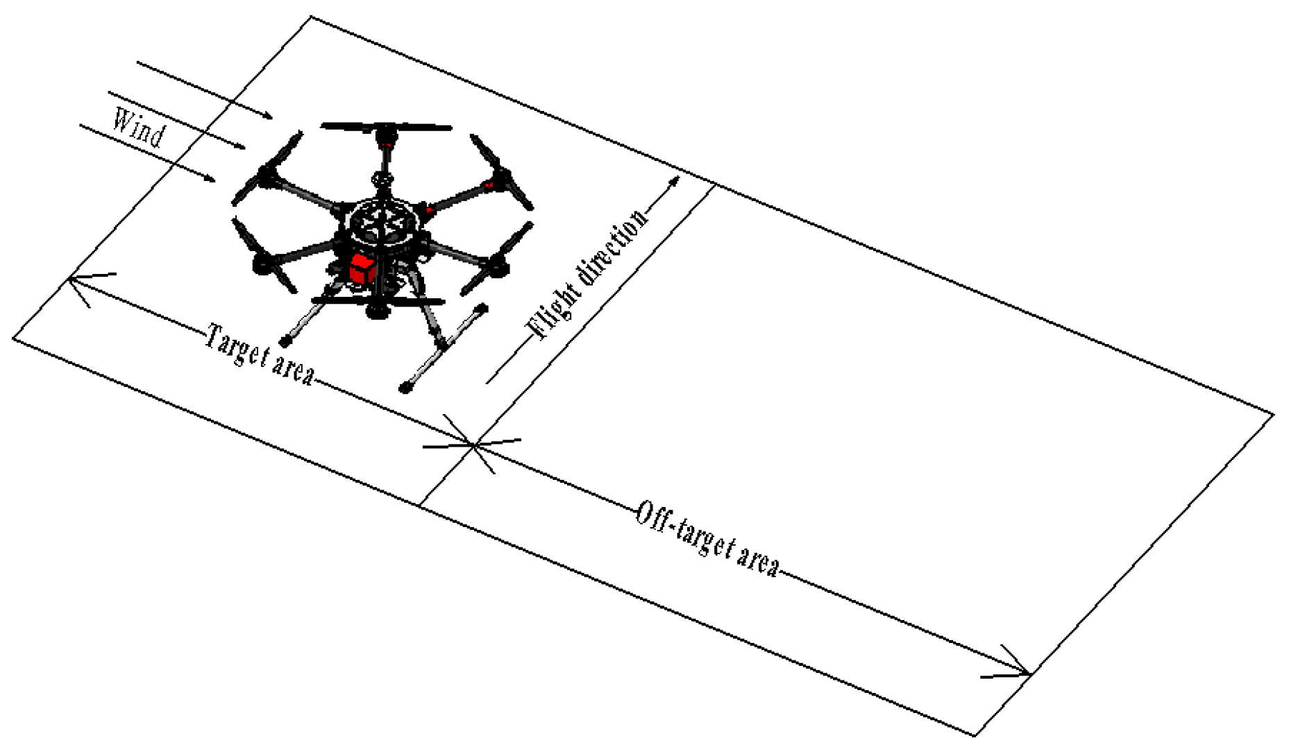
2.1. Geometric Model Building

According to the actual spray situation (Figure 1), a cuboid model is established in software ANSYS ICEM CFD15.0 (NASDAQ: ANSS, Canonsburg, PA, USA). The length and width of the simulation calculation area was set as 10 m and 4 m to simulate the spraying area, the height was set as 0.8 m, 1 m and 1.5 m to simulate the spraying heights, for total grid area of 228,000. The left side of the cuboid is an application target area, and the right side is a droplet drift (off-target) area. Grids in the target area are encrypted to have a better spatial resolution. The two nozzles are positioned directly above the center point of the target area (Figure 2).

The simulation analysis mainly obtains the droplet deposition rule and its influencing factor indexes. The boundary conditions are set as follows: The left face of the cuboid is the velocity inlet; the right face is the droplet receiving area pressure outlet; the other four surfaces are all pressure outlets; and the outlets are set as boundary escapes. According to the actual spraying operation height of the plant protection UAV, the sprayer height was changed to 0.8 m, 1 m and 1.5 m, respectively, by adjusting the position of the nozzles. The parameter settings are shown in

Table 1. Parameters of the flat fan atomizer used to simulate XR8002 nozzle.

Parameters (Unit)	Value
X-Center (m)	1.75/2.25
Y-Center (m)	2
Z-Center (m)	1.494
X-Virtual Center (m)	1.75/2.25
Y-Virtual Center (m)	2
Z-Virtual Center (m)	1.5
X-Fan Normal Vector	0
Y-Fan Normal Vector	−1
Z-Fan Normal Vector	1
Flow Rate (kg s−1)	0.01316
Spray Half Angle (deg)	40
Orifice Width (m)	0.00091
Flat Fan Sheet Constant	3
Atomizer Dispersion Angle (deg)	6

.

In the simulation analysis, the continuous phase substance is air and the discrete uses the parameters of liquid water to simulate chemical. In the steady-state calculation mode, the standard k-ε model (ANSYS, 15.0) [20,21] is selected to simulate the turbulent wind flow. Its transport equations are shown in Equations (1) and (2).

$$\frac{\partial \left(\rho k\right)}{\partial t}+\frac{\partial (\rho k{u}_i)}{\partial x_i}=\frac{\partial }{\partial x_j}[(\mu +\frac{{\mu }_t}{{\sigma }_k})\frac{\partial k}{\partial x_j}]+G_k+G_b-\rho \epsilon -Y_M+S_k$$

(1)

$$\frac{\partial \left(\rho \epsilon \right)}{\partial t}+\frac{\partial (\rho \epsilon u_i)}{\partial x_i}=\frac{\partial }{\partial x_j}[(\mu +\frac{{\mu }_t}{{\sigma }_{\epsilon }})\frac{\partial \epsilon }{\partial x_j}]+{\mathrm{C}}_{1\epsilon }\frac{\epsilon }{k}(G_k+C_{3\epsilon }{G}_b)-C_{2\epsilon }\rho \frac{{\epsilon }^2}{k}+S_{\epsilon }$$

(2)

where k is the turbulence kinetic energy, ε is the turbulence dissipation rate, μ is the dynamic viscosity, μ_t is the turbulence viscosity, $G_k$ is generated by turbulent kinetic energy caused by the average velocity gradient, and $G_b$ is generated by turbulent kinetic energy caused by buoyancy. $Y_M$ is a pulsating expansion term in compressible turbulence, $C_{1\epsilon }$, $C_{2\epsilon }$ and $C_{3\epsilon }$ are empirical constants, Prandtl numbers of ${\sigma }_k$ and ${\sigma }_{\epsilon }$ correspond to turbulent kinetic energy k and turbulent dissipation rate respectively, $S_k$ and $S_{\epsilon }$ is a user-defined source item.

The variation of air density under standard atmospheric pressure and normal temperature is less than 5%, it is regarded as an incompressible fluid, the pressure-based solver type is selected. All the simulations are based on the transient calculation. The convergence criterion is set to 10⁻⁵, which means that the converged solutions are reached when the residuals of several significant variables are equal to or less than 10⁻⁵.

2.2. Design of Experiment

As is shown in Figure 3, the spray effect is seriously affected by wind speed. The control variates method was used to solve the problem including multivariate by changing one of the factors. This study used different wind speeds, 0 m s⁻¹, 1 m s⁻¹, 3 m s⁻¹ and 5 m s⁻¹, to seek the law of droplet drift, and different particle mass flow rates, 0.01083 kg s⁻¹, 0.01316 kg s⁻¹ and 0.01516 kg s⁻¹, to control the spray pressure at 0.2 MPa, 0.3 MPa and 0.4 MPa, respectively. The overall control variates of the parameters are shown in

Table 2. Total variates of spray height (0.8, 1, and 1.5 m), pressure (0.2, 0.3, and 0.4 MPa) and wind speed (0, 1, 3, and 5 m s⁻¹).

Spray Height(m)	0.8			1			1.5
Pressure (MPa)	0.2	0.3	0.4	0.2	0.3	0.4	0.2	0.3	0.4
Wind Speed (m s−1)
0	A11	A12	A13	B11	B12	B13	C11	C12	C13
1	A21	A22	A23	B21	B22	B23	C21	C22	C23
3	A31	A32	A33	B31	B32	B33	C31	C32	C33
5	A41	A42	A43	B41	B42	B43	C41	C42	C43

.

The ability of DPM has been shown to accurately simulate particle dispersion and deposition [22,23,24]. In this study, the flat fan atomizer model of the DPM was selected to simulate the XR8002 nozzle of Teejet Company (Wheaton, IL, USA, 60187). In the DPM model, Euler method is used to describe the continuous phase. Navier-Stokes equation [25] is used to obtain velocity and other parameters. The discrete phase is described by Lagrange method, and its movement is obtained by integrating the motion equations of a large number of particles. Therefore, this model is called Euler-Lagrange model, and its transport equation can be expressed as [26]

$$\frac{d_{u_p}}{dt}=\frac{18\mu C_D{R}_e}{24{\rho }_p{dp}^2}(u-u_p)+\frac{g_x({\rho }_p-\rho )}{{\rho }_p}+\frac{1}{2}\frac{\rho }{{\rho }_p}\frac{d}{dt}(u-u_p)$$

(3)

where u is the continuous phase velocity, u_p is the velocity of particle, ρ_p is the density of particle, d_p is the particle diameter, g_x is the acceleration of gravity, R_e is the relative Reynolds number, and C_D is the drag coefficient.

2.3. Method of Analysis

In order to show the influence of three factors (wind speed, spray pressure, and spray height) on the droplet drift distance, deposition center drift distance, and overlap width, the multivariate curve fitting was carried out by the least square method [27,28]. The equation is listed as follows:

$${\mathrm{y}}_1{=\mathrm{a}}_0+{\mathrm{a}}_1{\mathrm{x}}_{\mathrm{w}}+{\mathrm{a}}_2{\mathrm{x}}_{\mathrm{p}}+{\mathrm{a}}_3{\mathrm{x}}_{\mathrm{h}}$$

(4)

$${\mathrm{y}}_2{=\mathrm{a}}_4+{\mathrm{a}}_5{\mathrm{x}}_{\mathrm{w}}+{\mathrm{a}}_6{\mathrm{x}}_{\mathrm{p}}+{\mathrm{a}}_7{\mathrm{x}}_{\mathrm{h}}$$

(5)

$${\mathrm{y}}_3{=\mathrm{a}}_8+{\mathrm{a}}_9{\mathrm{x}}_{\mathrm{w}}+{\mathrm{a}}_{10}{\mathrm{x}}_{\mathrm{p}}+{\mathrm{a}}_{11}{\mathrm{x}}_{\mathrm{h}}$$

(6)

Satisfy

$${\displaystyle \sum _{\mathrm{i}=1}^{\mathrm{n}}{(\mathrm{y}-{\mathrm{y}}_{\mathrm{i}})}^2}=\min {\displaystyle \sum _{\mathrm{i}=1}^{\mathrm{n}}{(\mathrm{y}-{\mathrm{y}}_{\mathrm{i}})}^2}$$

(7)

The model obtained by the least square method can be verified by Equation (8),

$${\mathrm{y}}_{\mathrm{o}}{=\mathrm{a}}_0-{\mathrm{y}}_{\mathrm{n}}+{\mathrm{y}}_{\mathrm{f}}$$

(8)

where y_o is the overlap width influenced by wind, a_o is the overlap width in nature, y_n is the drift distance of near tuyere edge, and y_f is the drift distance of far tuyere edge. Their relationship can be portrayed in Figure 4.

3. Results and Discussion

3.1. Simulation of Influence of Different Factors on Droplet Drift

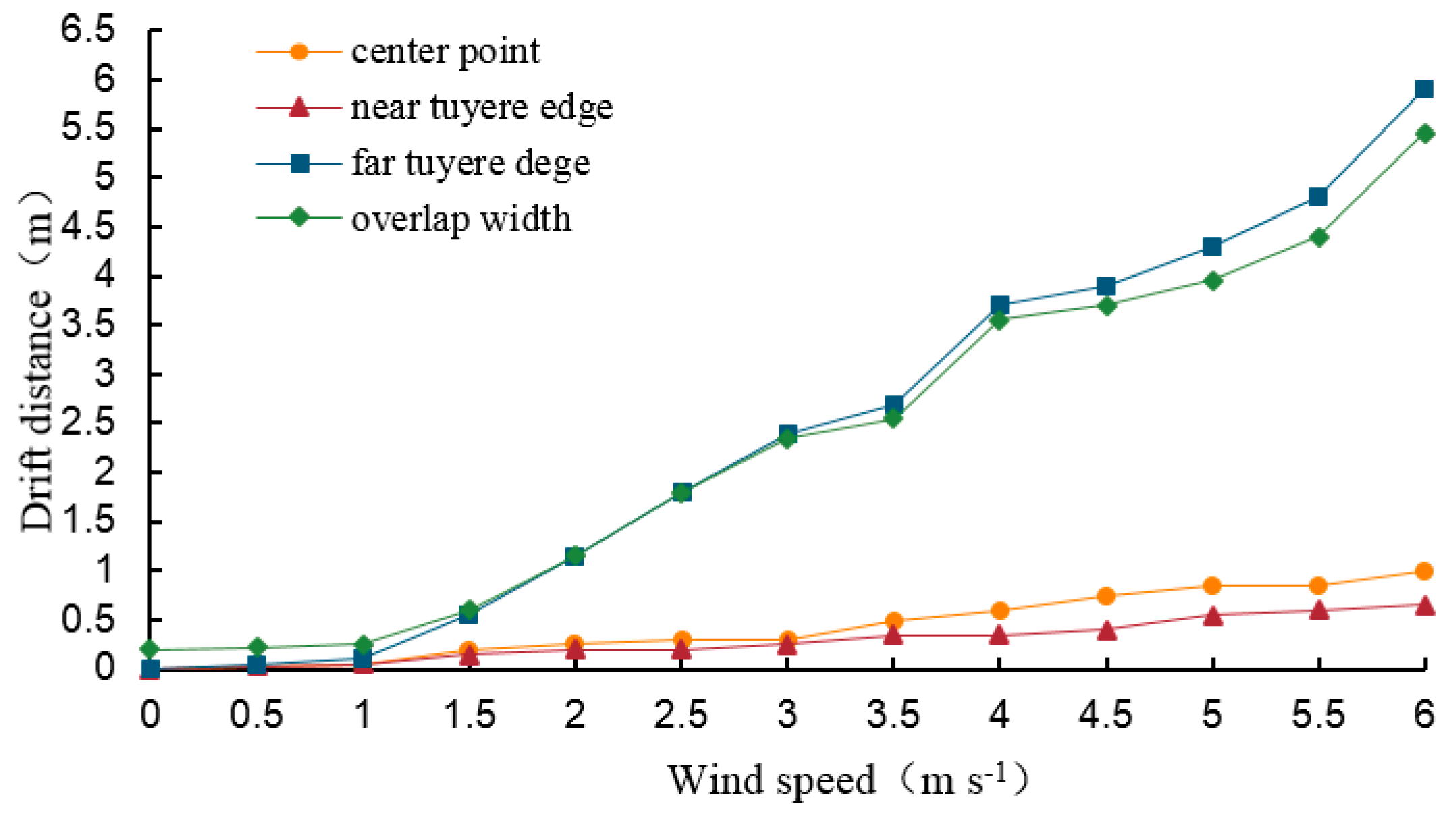
3.1.1. Influence of Wind Speed on Droplet Drift

Inlet pressure (0.3 MPa) and spray height (1.5 m) were set to constant and the effect of ambient wind speeds of 0 m s⁻¹, 1 m s⁻¹, 3 m s⁻¹, and 5 m s⁻¹ were explored. The droplet deposition density at different target positions is plotted in Figure 5.

It is clear that droplet deposition concentration at different target locations varied with wind speed (Figure 5). When the wind speed was 0 m s⁻¹, the droplets did not drift. The droplet concentration deposition center point was 2 m and the drift distance was 0. When the wind speed was 1 m s⁻¹, the droplet had a minor drift phenomenon. The droplet concentration deposition center point was 2.05 m and the drift distance was 0.05 m. When the wind speed was 3 m s⁻¹, the droplet had obvious drift phenomenon. The droplet concentration deposition center point was 2.35 m and the drift distance was 0.35 m. When the wind speed was 5 m s⁻¹, the droplets had a large amount of drift. The droplet concentration deposition center point was 2.85 m and the drift distance was 0.85 m. The three main performance indicators to evaluate drift characteristics, drift distance of deposition center, near tuyere edge, and far tuyere edge, and the relationships between these parameters and wind speed are shown in

Table 3. Droplet drift distance of deposition center, near tuyere edge, far tuyere edge, and overlap width at different wind speed, 0 m s⁻¹, 1 m s⁻¹, 3 m s⁻¹ and 5 m s⁻¹.

Wind Speed (m s−1)	Deposition Center (m)	Near Tuyere Edge (m)	Far Tuyere Edge (m)	Overlap Width (m)
0	0	0	0	0.20
1	0.05	0.05	0.05	0.65
3	0.45	0.25	2.40	2.35
5	0.85	0.55	4.60	3.95

and Figure 6.

The least square method was used to fit the drift distance and overlap width under different wind speeds. The center point drift model was y₁ = 0.176x_w + 0.091, near tuyere edge drift model was y₂ = 0.110x_w − 0.038, far tuyere edge drift model was y₃ = 1.016x_w − 0.636, and the overlap width model was y₄ = 0.901x_w − 0.382. In these models, x_w was wind speed (m s⁻¹) and y was distance (m). It can be seen that the wind speed was positively correlated with drift distance and overlap width. For every 1 m s⁻¹ increase in wind speed, drift distance of droplet center point was increased by 0.176 m, near tuyere edge was increased by 0.11 m, far tuyere edge was increased by 1.016 m, and overlap width was increased by 0.901 m. The accuracy can be verified by the model obtained above with a₀ representing the droplet overlap width in the natural state. The simulation showed that when a₀ = 0.2, y₄ − (a₀ − y₂ + y₃) = 0.005x + 0.0156 was about 0, which proved that the model fits the actual situation.

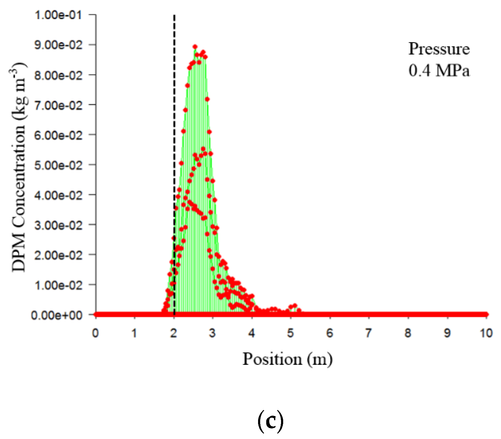
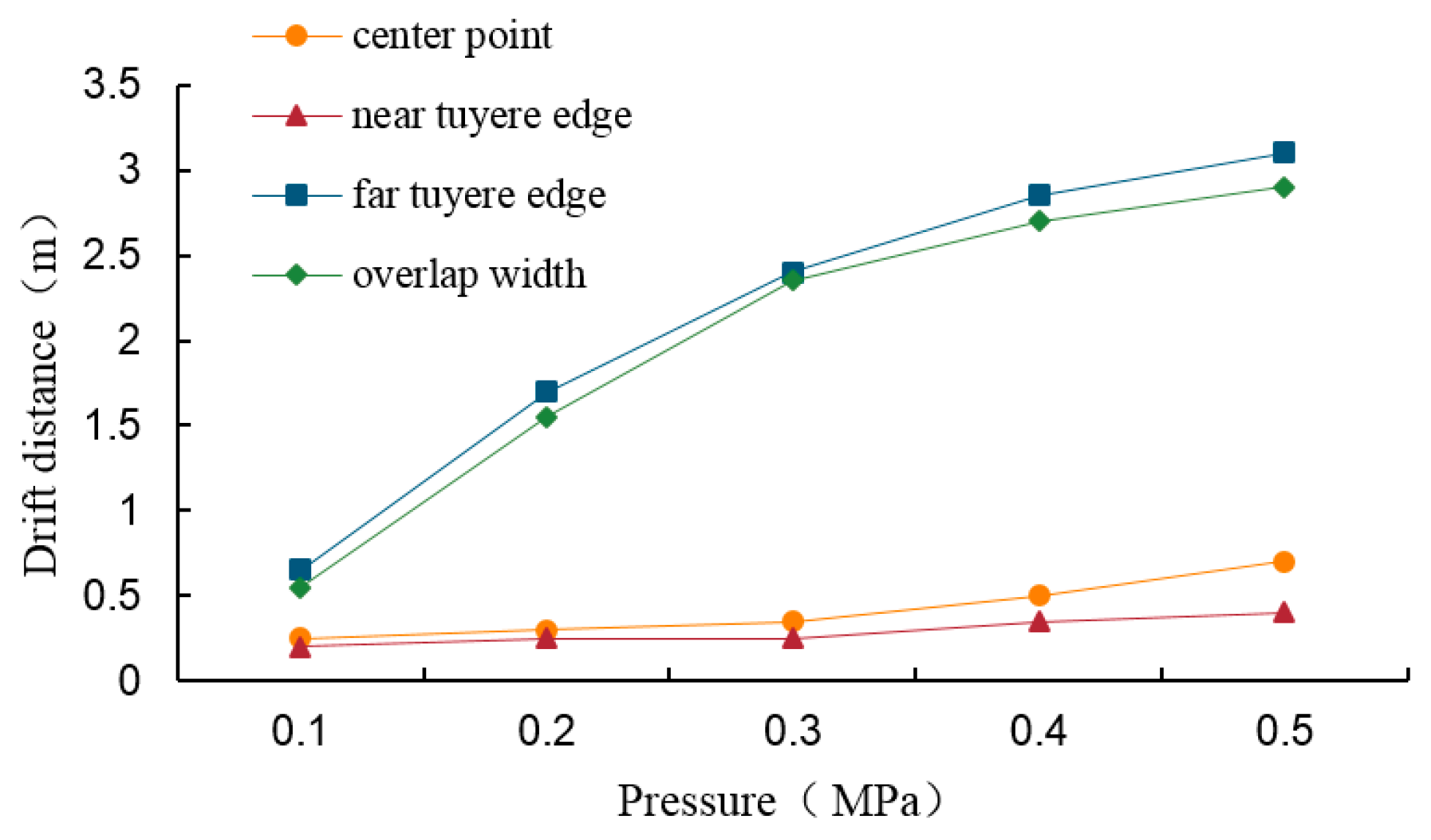
3.1.2. Influence of Inlet Pressure on Droplet Drift

Wind speed (3 m s⁻¹) and spray height (1.5 m) were set to constant and the pressure of 0.2 MPa, 0.3 MPa and 0.4 MPa was explored. The droplet deposition density at different target positions is plotted in Figure 7.

It is clear that droplet deposition concentration at different target locations varies under the influence of pressure (Figure 7). When the pressure was 0.2 MPa, the droplet concentration deposition center point is 2.35 m and the drift distance is 0.35 m. When the pressure was 0.3 MPa, the droplet concentration deposition center point is 2.45 m and the drift distance is 0.45 m. When the pressure was 0.4 MPa, the droplet concentration deposition center point is 2.6 m and the drift distance is 0.6 m. The drift distance of deposition center, the edge of near tuyere, and the edge of far tuyere and the relationships between these parameters and pressure are shown in

Table 4. Droplet drift distance of deposition center, near tuyere edge, far tuyere edge, and overlap width under different pressure, 0.2 MPa, 0.3 MPa, and 0.4 MPa.

Pressure (MPa)	Deposition Center (m)	Near Tuyere Edge (m)	Far Tuyere Edge (m)	Overlap Width (m)
0.2	0.60	0.25	1.70	1.55
0.3	0.45	0.25	2.40	2.35
0.4	0.65	0.35	2.85	2.70

and Figure 8.

The least square method was used to fit the drift distance and overlap width under different wind speeds. The center point drift model is y₅ = 0.110x_p + 0.090, the near tuyere edge drift model is y₆ = 0.050x_p + 0.140, the far tuyere edge drift model is y₇ = 0.605x_p + 0.325, and the overlap width model is y₈ = 0.601x_p + 0.600. In the models, x is inlet pressure (MPa) and y is distance (m). It can be seen that inlet pressure is positively correlated with droplet drift distance and overlap width. For every 0.1 MPa increased in the inlet pressure, the drift distance of deposition center point was increased by 0.11 m, the edge of near tuyere was increased by 0.05 m, the edge of far tuyere was increased by 0.605 m, and the overlap width was increased by 0.6 m.

3.1.3. Influence of Spray Height on Droplet Drift

Wind speed (3 m s⁻¹) and pressure (0.3 MPa) were set to constant and the spray height of 0.8 m, 1 m, and 1.5 m was explored. The droplet deposition density at different target positions is plotted in Figure 9.

It is clear that droplet deposition concentration at different target locations varied with spray height (Figure 9). When the spray height was 0.8 m, the droplet concentration deposition center point is 2.35 m and the drift distance is 0.35 m. When the spray height was 1 m, the droplet concentration deposition center point is 2.45 m and the drift distance is 0.45 m. When the spray height was 1.5 m, the droplet concentration deposition center point is 2.6 m and the drift distance is 0.6 m. The deposition center, near tuyere edge, and far tuyere edge, and the relationship between these parameters and spray height are shown in

Table 5. Droplet drift distance of deposition center, near tuyere edge, far tuyere edge, and overlap width in different spray height, 0.8 m, 1 m, and 1.5 m.

Spray Height (m)	Deposition Center (m)	Near Tuyere Edge (m)	Far Tuyere Edge (m)	Overlap Width (m)
0.8	0.35	0.15	1.55	1.35
1	0.45	0.25	2.40	2.60
1.5	0.60	0.35	3.25	2.75

and Figure 10.

Again, the least square method was used to fit the drift distance and overlap width under different spray heights. The center point drift model is y₉ = 0.235x_h + 0.125, the near tuyere drift model is y₁₀ = 0.115x_h + 0.902, the far tuyere drift model is y₁₁ = 1.654x_h − 0.081, and the overlap width is y₁₂ = 1.670x_h + 0.789. In the models, x is the spray height (m) and y is the distance (m). It can be seen that the spray height is positively correlated with droplet drift distance and overlap width, i.e., for every 1m increase in spray height, the drift distance of deposition center point was increased by 0.235 m, the drift distance of near tuyere increased by 0.115 m, the drift distance of far tuyere was increased by 1.654 m, and the overlap width was increased by 1.67 m.

3.2. Drift Distance Analysis of Fitting Regression Results

The least square method was taken to fit a curve of drift, with y₁ (edge drift distance), y₂ (deposition center drift distance), and y₃ (overlap width) as dependent variables, and x_w (wind speed), x_p (inlet pressure), and x_h (spray height) as independent variables, and C (constant term). The corresponding equations of multivariate linear function groups can be explained as follows:

$$\left(\begin{array}{cccc}\begin{array}{l}27\\ 81\\ 89.1\\ 29.7\end{array}& \begin{array}{c}81\\ 315\\ 243\\ 89.1\end{array}& \begin{array}{c}81\\ 243\\ 288\\ 89.1\end{array}& \begin{array}{c}29.7\\ 89.1\\ 89.1\\ 35\end{array}\end{array}\right)\left(\begin{array}{l}{\mathrm{a}}_0\\ {\mathrm{a}}_1\\ {\mathrm{a}}_2\\ {\mathrm{a}}_3\end{array}\right)=\left(\begin{array}{c}57.025\\ 243.925\\ 180.975\\ 66.36\end{array}\right)$$

(9)

$$\left(\begin{array}{cccc}\begin{array}{l}27\\ 81\\ 89.1\\ 29.7\end{array}& \begin{array}{c}81\\ 315\\ 243\\ 89.1\end{array}& \begin{array}{c}81\\ 243\\ 288\\ 89.1\end{array}& \begin{array}{c}29.7\\ 89.1\\ 89.1\\ 35\end{array}\end{array}\right)\left(\begin{array}{l}{\mathrm{a}}_0\\ {\mathrm{a}}_1\\ {\mathrm{a}}_2\\ {\mathrm{a}}_3\end{array}\right)=\left(\begin{array}{c}11.5\\ 46.5\\ 36.025\\ 13.37\end{array}\right)$$

(10)

$$\left(\begin{array}{cccc}\begin{array}{l}27\\ 81\\ 89.1\\ 29.7\end{array}& \begin{array}{c}81\\ 315\\ 243\\ 89.1\end{array}& \begin{array}{c}81\\ 243\\ 288\\ 89.1\end{array}& \begin{array}{c}29.7\\ 89.1\\ 89.1\\ 35\end{array}\end{array}\right)\left(\begin{array}{l}{\mathrm{a}}_0\\ {\mathrm{a}}_1\\ {\mathrm{a}}_2\\ {\mathrm{a}}_3\end{array}\right)=\left(\begin{array}{l}51.475\\ 204.275\\ 172.5\\ 60.06\end{array}\right)$$

(11)

and solved by MATLAB 2015a® (MathWorks, MA, USA),

$${\left({\mathrm{a}}_0{\mathrm{a}}_1{\mathrm{a}}_2{\mathrm{a}}_3\right)}^{\mathrm{T}}={\left(-3.0960.8870.5501.552\right)}^{\mathrm{T}}$$

(12)

$${\left({\mathrm{a}}_0{\mathrm{a}}_1{\mathrm{a}}_2{\mathrm{a}}_3\right)}^{\mathrm{T}}={\left(-0.6670.1670.0850.308\right)}^{\mathrm{T}}$$

(13)

$${\left({\mathrm{a}}_0{\mathrm{a}}_1{\mathrm{a}}_2{\mathrm{a}}_3\right)}^{\mathrm{T}}={\left(-3.3740.6920.5291.469\right)}^{\mathrm{T}}$$

(14)

Table 6. The variance and regression analysis of the influence of three factors on edge drift distance, deposition center drift distance, and overlap width analysis.

Dependent Variable	Source of Difference	Regression Coefficient	T-Distribution Value	Significance	95% Confidence Interval		R	R2
					Lower Limit	Upper Limit
Y1	Xw	0.887	9.941	**	0.702	1.071	0.915	0.837
	Xp	0.550	3.083	*	0.181	0.919
	Xh	1.552	3.137	*	0.529	2.576
	C	−3.096	−4.752		−5.606	−2.206
Y2	Xw	0.167	8.196	**	0.125	0.209	0.880	0.774
	Xp	0.085	2.083	*	0.001	0.169
	Xh	0.308	2.728	*	0.074	0.541
	C	−0.667	−3.558		−1.054	−0.279
Y3	Xw	0.692	8.303	**	0.520	0.865	0.892	0.795
	Xp	0.529	3.173	*	0.184	0.874
	Xh	1.469	3.176	*	0.512	2.426
	C	−3.374	−4.391		−4.963	−1.785

The dependent variables (Y₁, Y₂, Y₃) are edge drift distance, deposition center drift distance, and overlap width. The different sources (X_w, X_p, X_h, C) are wind speed, inlet pressure, spray height and constant term. The significances are the results of significance analysis and the number of stars means the degree of influence by independent variables. The two stars (**) means the influence is very significant, one star (*) is significant, and no star is not significant.

shows the variance and regression analysis of the influence of three factors on edge drift distance, deposition center drift distance and overlap width. According to the analysis results (Table 6), the influence of wind speed on edge drift distance, deposition center drift distance and overlap width is very significant, pressure and spray height is significant. The influence of three factors on edge drift distance, deposition center drift distance, and overlap width is also significant, so a linear equation can be established.

The regression coefficients of the three variables in the regression equation of edge drift distance are 0.887, 0.550, and 1.552, and the constant term (C) is −3.096. Therefore, the relationship model between edge drift distance Y₁ and wind speed X_w (m s⁻¹), pressure X_p (MPa) and spray height X_h (m) is

Y₁ = 0.887X_w + 0.550X_p + 1.552X_h − 3.906 (R² = 0.837)

(15)

In this model (15), the coefficients of the three variables are all positive, indicating that the three factors are all positively correlated with droplet drift distance of far tuyere edge. At the same time, this model also provides a reference for safe distance. This model is the drift distance of the droplet far from far tuyere edge, which is also the farthest distance to which the droplet can drift.

The regression coefficients of the three variables in the regression equation of center drift distance are 0.167, 0.085, and 0.308, and the C is −0.667. Therefore, the relationship model between drift distance Y₂ of deposition center and wind speed X_w (m s⁻¹), pressure X_p (MPa) and spray height X_h (m) is

Y₂ = 0.167X_w + 0.085X_p + 0.308X_h − 0.667 (R² = 0.774)

(16)

In this model (16), the coefficients of the three variables are all positive, indicating that the three factors are positively correlated with the drift distance of droplet deposition center. At the same time, this model also provides a reference for the selection of spray deposition center. This model is the drift distance of droplet deposition center, which is also the point where droplet deposition concentration is the largest.

The regression coefficients of the three variables in the regression equation of overlap width are 0.692, 0.529, and 1.469, and the C is −3.374. Therefore, the relationship model between overlap width Y₃ and wind speed X_w (m s⁻¹), pressure X_p (MPa), and spray height X_h (m) is

Y₃ = 0.692x_w + 0.529x_p + 1.469x_h − 3.374 (R² = 0.795)

(17)

In this model (17), the coefficients of the three variables are all positive, indicating that the three factors are positively correlated with the overlap width. At the same time, this model also provides a reference for the selection of nozzle distance and how to get the best droplet overlapping effect.

3.3. Analysis of Droplet Drift Curve Characteristic

Under the influence of different wind speeds, the droplet drift curve of XR8002 (spray height 1.5 m; inlet pressure 0.3 MPa) is shown in Figure 11.

As can be seen from the above Figure 11, when the wind speed was 1 m s⁻¹, the droplets hardly drift. When the wind speed exceeded 1 m s⁻¹, the droplets drift slightly. When the wind speed exceeded 3 m s⁻¹, the droplets will obviously drift. It is also the reason why UAV could not work in high wind speed. The analysis of droplet drift curves at the wind speeds of 3 m s⁻¹ and 5 m s⁻¹ were also made in Figure 12.

As is shown in Figure 12, both sides of the droplet drift curve were approximately a straight line. When the wind speed was 3 m s⁻¹, the droplet angle on the left side was 90°and the right side was 20.67°. When the wind speed was 5 m s⁻¹, the droplet angle on the left side was 70.42°and the right side was 11.27°, which showed that the inclination angle of the straight line was negatively related to the wind speed. Results displayed in Figure 12 show trends matching the previously observed behavior of a drift distance increase with a droplet angle decrease. The droplet angle also could be used to estimate the influence of wind, and the drift distance.

4. Conclusions

In this study, CFD simulation method was used to acquire droplet deposition distribution and drift under the influence of different factors. DPM model was used to simulate droplet drift from a double XR8002 nozzle at various wind speeds (0, 1, 3, 5 m s⁻¹), nozzle pressures (0.2, 0.3, 0.4 MPa) and spray heights (0.8, 1, 1.5 m). The information obtained from these simulations provided valuable insight into the characteristic of spray drift. General analysis suggest that the droplet drift curves were influenced by the three factors. Additionally, the influence coefficients of the three factors on the droplet drift distance were calculated. On the basis of analysis of the variance and regression results aimed at the edge drift distance, the center drift distance, and the overlap width, the three models were established. The expressions of three models are important on guiding significance to the practice. The analysis of the droplet drift curves showed that the droplet angle is closely related to drift. Results made from these simulations have provided a tool which can be used to ensure future UAV chemical application can be designed to maximize efficacy, reduce waste, and minimize damage to organisms not being targeted.

References

1. Han, H.Q.; Gao, H.J.; Yang, H.T.; Zhang, X.; Hu, T.; Zhou, Q.Q. Analysis on decoupling between total grain production and pesticide usage in China. Subtrop. Agric. Res. 2018, 14, 91–98. [Google Scholar]
2. Cheng, X.B. Current situation and development countermeasures of agricultural extension in China. Agric. Sci. Technol. 2018, 23, 255–259. [Google Scholar]
3. Wu, K.M.; Lu, Y.H.; Wang, Z.Y. Advance in integrated pest management of crops in China. Chin. Bull. Entomol. 2009, 46, 831–836. [Google Scholar]
4. Wang, G.; Gong, Y.; Zhang, X.; Chen, X.; Liu, D.J.; Chen, W.; Miao, Y.Y. The test of droplet deposition distribution for different kinds of pesticide application equipment in corn field. J. Agric. Mech. Res. 2017, 39, 177–182. [Google Scholar]
5. Meng, Y.H.; Zhou, G.Q.; Wu, C.B. Discussion on application and promotion of agricultural plant protection unmanned aerial vehicle in China. China Plant Prot. 2014, 34, 33–39. [Google Scholar]
6. Shang, C.Y.; Cai, J.F.; Huang, S.J.; Pan, H.L.; Zhong, F.L. Applications status and prospect analysis of agricultural UAVs in China. J. Anhui Agric. Sci. 2017, 45, 193–195. [Google Scholar]
7. Wang, X.N.; He, X.K.; Wang, C.L.; Wang, Z.C.; Li, L.L.; Wang, S.L.; Janes, B.; Andreas, H.; Wang, Z.G. Spray drift characteristics of fuel powered single-rotor UAV for plant protection. Trans. Chin. Soc. Agric. Eng. 2017, 33, 117–123. [Google Scholar]
8. Bradley, K.F. Role of atmospheric stability in drift and deposition of aerially applied sprays-preliminary results. ASAE 2004, 58, 742–755. [Google Scholar]
9. Kirk, L.W.; Teske, M.E.; Thistle, H.W. What about upwind buffer zones for aerial applications? J. Agric. Saf. Health 2002, 8, 333–336. [Google Scholar] [CrossRef]
10. Ivan, W.K.; Bradley, K.F.; Wesley, C.H. Aerial methods for increasing spray deposits on wheat heads. ASAE 2004, 58, 716–729. [Google Scholar]
11. Chen, S.D.; Lan, Y.B.; Bradley, K.F. Effect of wind Field below Rotor on Distribution of Aerial Spraying Droplet Deposition by Using Multi-rotor UAV. Trans. Chin. Soc. Agric. Mach. 2017, 48, 105–113. [Google Scholar]
12. Qiu, B.J.; Wang, L.W.; Cai, D.L.; Wu, J.H.; Ding, G.R.; Guan, X.P. Effects of flight altitude and speed of unmanned helicopter on spray deposition uniform. Trans. Chin. Soc. Agric. Mach. 2013, 29, 25–32. [Google Scholar]
13. Shen, A.; Zhou, S.D.; Wang, M. Simulation and analysis of multi-rotor UAV flow field. Trans. Chin. Soc. Agric. Mach. 2018, 36, 29–33. [Google Scholar]
14. Nuyttens, D.; De Schampheleire, M.; Baetens, K.; Brusselman, E.; Dekeyser, D.; Verboven, P. Drift from field crop sprayers using an integrated approach: Results of a 5-year study. Trans. ASABE 2011, 54, 403–408. [Google Scholar] [CrossRef]
15. Teske, M.E.; Bird, S.L.; Esterly, D.M.; Curbishley, T.B.; Ray, S.L.; Perry, S.G. AgDrift: A model for estimating near-field spray drift from aerial applications. Environ. Toxicol. Chem. 2002, 21, 659–671. [Google Scholar] [CrossRef] [PubMed]
16. Teske, M.E.; Thistle, H.W.; Riley, C.M.; Hewitt, A.J. Laboratory measurements on the sensitivity of evaporation rate of droplets inside a spray cloud. Trans. ASABE 2017, 60, 361–366. [Google Scholar]
17. Bilanin, A.J.; Teske, M.E.; Barry, J.W.; Ekblad, R.B. AGDISP: The aircraft spray dispersion model, code development and experimental validation. Trans. ASABE 1989, 32, 327–334. [Google Scholar] [CrossRef]
18. Luo, J.; Zeng, G.H.; Li, B.K. Simulation analysis of two-phase flow field inside pass of nozzle base on FLUENT. Modul. Mach. Tool Autom. Manuf. Tech. 2016, 10, 44–47. [Google Scholar]
19. Chen, X.; Ge, S.C.; Zhang, Z.W.; Jing, D.J. Numerical simulation and analysis of multi-nozzle interference base on fluent. Chin. J. Environ. Eng. 2014, 8, 2503–2508. [Google Scholar]
20. Sun, G.X.; Wang, X.C.; Ding, W.M.; Zhang, Y. Simulation and analysis on characteristics of droplet deposition base on CFD discrete phase model. Trans. Chin. Soc. Agric. Eng. 2012, 28, 13–19. [Google Scholar]
21. Zhang, S.F.; Song, L.L. Simulation of Spray characteristics of pressure swirl nozzle. J. Anhui Agric. Sci. 2009, 37, 8098–8100. [Google Scholar]
22. Adeniyi, A.A.; Morvan, H.P.; Simmons, K.A. A coupled Euler-Lagrange CFD modelling of droplets-to-film. Aeronaut. J. 2017, 121, 1897–1918. [Google Scholar] [CrossRef]
23. Ryan, S.D.; Gerber, A.G.; Holloway, A.G.L. A computational study on spray dispersal in the wake of an aircraft. Trans. ASABE 2013, 56, 847–868. [Google Scholar]
24. Zhang, B.; Tang, Q.; Chen, L.P.; Xu, M. Numerical simulation of wake vortices of crop spraying aircraft close to the ground. Biosyst. Eng. 2016, 145, 52–64. [Google Scholar] [CrossRef]
25. Yang, F.B.; Xue, X.Y.; Cai, C. Numerical Simulation and analysis on spray drift movement of multirotor plant protection unmanned aerial vehicle. Energies 2018, 11, 2399. [Google Scholar] [CrossRef]
26. Roberts, T.W.; Murman, E.M. Solution method for a hovering helicopter rotor using the Euler equations. In Proceedings of the 23rd Aerospace Sciences Meeting, Reno, NV, USA, 14–17 January 1985. [Google Scholar]
27. Jin, Y.H.; Jae, S.R.; Kyu, H.K. New least squares method with geometric conservation law (GC-LSM) for compressible flow computation in meshless method. Comput. Fluids 2018, 172, 122–146. [Google Scholar]
28. Salazar-Campoy, M.M.; Morales, R.D.; Najera-Bastida, A.; Calderon-Ramos, I.; Cedillo-Hernandez, V.; Delgado-Pureco, J.C. A physical model to study the effects of nozzle design on dispersed two-phase flows in a slab mold casting ultra-low-carbon steels. Metall. Mater. Trans. B 2018, 49, 812–830. [Google Scholar] [CrossRef]
Figure 1. The sketch of UAV, wind and flight direction is shown in diagram to simulate the actual spray picture. The target area is set under the UAV and the off-target area is set down wind relative to the UAV.
Agronomy 09 00308 g001
Figure 2. Computational domain and boundary setup are shown. The two nozzles are positioned on top of the domain.
Agronomy 09 00308 g002
Figure 3. Droplets deposition in target area at different wind speed (0 m s−1 and 3 m s−1). (a) The distribution of droplets is ideal at 0 m s−1, (b) The droplet was influenced by wind clearly and the distribution of droplets is not satisfied at 3 m s−1.
Agronomy 09 00308 g003
Figure 4. The natural curve of droplets is shown by solid lines and the drift curve influenced by wind is shown by dotted lines, a0 is overlap width, y2 is the drift distance of near tuyere edge, y3 is the drift distance of far tuyere edge, and y4 is the overlap width influenced by wind.
Agronomy 09 00308 g004
Figure 5. Concentration of droplets deposition at different wind speeds, (a) 0 m s−1, (b) 1 m s−1, (c) 3 m s−1, and (d) 5 m s−1. X-axis indicates a different position of target area and off-target area. Y-axis shows DPM concentration (kg m−3) of droplets deposition at different wind speeds, 0 m s−1, 1 m s−1, 3 m s−1, and 5 m s−1. The point means concentration of different position, the dotted line means the droplet concentration deposition center, and the solid line means the biggest concentration of corresponding point.
Agronomy 09 00308 g005
Figure 6. The relationship between wind speed and drift distance (center point, near tuyere edge, far tuyere edge, and overlap width).
Agronomy 09 00308 g006
Figure 7. Concentration of droplets deposition under different pressures, (a) 0.2 MPa, (b) 0.3 MPa, and (c) 0.4 MPa. X-axis indicates different position of target area and off-target area, Y-axis shows DPM Concentration (kg m−3) of droplets deposition under different pressure, 0.2 MPa, 0.3 MPa, and 0.4 MPa. The point means concentration of different position, the dotted line means the droplet concentration deposition center, and the solid line means the biggest concentration of corresponding point.
Agronomy 09 00308 g007aAgronomy 09 00308 g007b
Figure 8. The relationship between pressure and drift distance (center point, near tuyere edge, far tuyere edge and overlap width).
Agronomy 09 00308 g008
Figure 9. Concentration of droplets deposition in different spray heights, (a) 0.8 m, (b) 1 m, and (c) 1.5 m. X-axis means different position of target area and off-target area, Y-axis means DPM Concentration (kg m−3) of droplets deposition in different spray height, 0.8 m, 1 m, and 1.5 m. The point means concentration of different position, the dotted line means the droplet concentration deposition center and the solid line means the biggest concentration of corresponding point.
Agronomy 09 00308 g009
Figure 10. The relationship between spray height and drift distance (center point, near tuyere edge, far tuyere edge, and overlap width).
Agronomy 09 00308 g010
Figure 11. Trace of droplet drift curve at wind speed 0, 1, 3, and 5 m s−1 when spray height was 1.5 m and inlet pressure was 3 MPa. (a) The droplets have no drift at 0 m s−1, (b) The droplets hardly drift at 1 m s−1, (c) The droplets have obvious drift at 3 m s−1, (d) The droplets have serious drift at 5 m s−1.
Agronomy 09 00308 g011
Figure 12. Droplet drift curve of different wind speed (3 and 5 m s−1), X-axis means deposition area of 0 to 10m, and Y-axis means spray height. (a) The droplet angle was 90° and 20.67° at 3 m s−1, (b) The droplet angle was 70.42° and 11.27° at 5 m s−1.
Agronomy 09 00308 g012