Simulating Growth and Development Processes of Quinoa (Chenopodium quinoa Willd.): Adaptation and Evaluation of the CSM-CROPGRO Model

Abstract

In recent years, the intra-annual yield variability of traditional food crops grown in Europe increased due to extreme weather events driven by climate change. The Andean crop quinoa (Chenopodium quinoa Willd.), being well adapted to drought, salinity, and frost, is considered to be a promising new crop for Europe to cope with unfavorable environmental conditions. However, cultivation guidelines and cropping experiences are missing on a long-term scale. The adaptation of a mechanistic crop growth model will support the long-term evaluation of quinoa if grown under the diverse environmental conditions of Europe. The objective of this study was to adapt the process-based cropping system model (CSM) CROPGRO, which is included in the Decision Support System for Agrotechnology Transfer (DSSAT). Therefore, species and genetic coefficients were calibrated using literature values and growth analysis data, including crop life cycle, leaf area index (LAI), specific leaf area (SLA), dry matter partitioning and nitrogen concentrations in different plant tissues, aboveground biomass, and yield components, of a sowing date experiment (covering two cultivars and four sowing dates) conducted in southwestern Germany in 2016. Model evaluation was performed on the crop life cycle, final aboveground biomass, and final grain yield for different sowing dates using an independent data set collected at the same site in 2017. The resulting base temperatures regarding photosynthetic, vegetative, and reproductive processes ranged between 1 and 10 °C, while the corresponding optimum temperatures were between 15 and 36 °C. On average, the crop life cycle was predicted with a root mean square error (RMSE) of 4.7 and 3.0 days in 2016 and 2017, respectively. In 2016, the mean predicted aboveground biomass during the growth cycle showed a d-index of 0.98 (RMSE = 858 kg ha⁻¹). Furthermore, the LAI, SLA, and leaf nitrogen concentrations were simulated with a high accuracy, showing a mean RMSE of 0.29 (d-index = 0.94), 25 cm² g⁻¹ (d-index = 0.88), and 0.51% (d-index = 0.95). Evaluations on the grain yield and aboveground biomass across four sowing dates in 2017 suggested a good robustness of the new quinoa model. The mean predicted aboveground biomass and grain yield at harvest maturity were 6479 kg ha⁻¹ (RMSE = 898.9 kg ha⁻¹) and 3843 kg ha⁻¹ (RMSE = 450.3 kg ha⁻¹), respectively. Thus, the CSM-CROPGRO model can be used to evaluate the long-term suitability, as well as different management strategies of quinoa under European conditions. However, further development on the simulation of small seed sizes and under water or nitrogen-limited environments are needed.

1. Introduction

Besides general effects, such as global warming or increased atmospheric CO₂ concentrations in the atmosphere, the progressing climate change includes extreme weather events like heat waves, increased frequencies of drought, and higher rainfall intensities during wet phases. As a consequence of climate change, the cultivation of traditional food crops in Europe suffers from increased yield variability, which could become a serious problem not only for farmers’ income, but also for food security [1,2]. To minimize the negative impacts of climate change on food production, new strategies in terms of crop management, e.g., differing sowing and harvest dates, new tillage practices for soil water conservation, or precision farming strategies regarding crop protection and fertilization, are needed [3]. Further possible strategies are also the substitution of traditionally cultivated crops that show a high inter-annual yield variability or the inclusion of new species that are tolerant against abiotic stresses to diversify conventional crop rotations [1,4,5,6]. Quinoa (Chenopodium quinoa Willd.) is considered a potential new crop for Europe to deal with unfavorable environmental conditions [7]. Quinoa originates from the Andean region, including Bolivia, Peru, Chile, Ecuador, and Argentina [8,9]. Due to widely differing agro-ecological conditions (soils, rainfall, temperatures, and altitudes) within the natural habitats of these countries, quinoa developed a broad genetic diversity, which led to tolerances against various abiotic stress factors [8,10,11,12]. Among others, quinoa was shown to be well adapted to (semi-)arid conditions [13,14], salinity [14,15], and frost [16]. Furthermore, the annual dicotyledonous, herbaceous crop of the Amaranthaceae family produces gluten-free cereal-grain-like achenes, which show considerable concentrations of high-quality proteins (containing all essential and semi-essential amino acids) and nutritionally favorable lipids [8,17,18]. Due to these healthy nutritional properties, the world-wide demand for quinoa has grown rapidly in recent years, which was accompanied by rapid price increases [19,20]. Thus, quinoa could also be used as a cash-crop by European farmers to compensate for financial losses caused by the upcoming yield variability of traditional crops.

Despite the successful experimental cultivation of quinoa in several parts of Europe [17,21,22,23,24], the introduction of a new crop requires expensive multi-location long-term studies to evaluate its adaptability and suitable management practices [25,26,27]. Therefore, in recent years, potential interactions between the genotype and environment of different crops have been investigated more frequently with the help of mechanistic crop growth simulation models [28,29,30,31,32]. Furthermore, crop growth models can be used to support decision-making since there is a possibility of evaluating potential growth limitations induced by different management scenarios [33,34]. Due to its exceptional capabilities regarding possible growth conditions combined with a great nutritive value, the research interest in modeling quinoa growth and development has increased continuously over the last few years [35,36,37,38,39,40,41]. Nevertheless, until now, only the physically based, water-driven crop growth models AquaCrop [42] and SALTMED [43,44] have been parameterized to simulate quinoa growth. While appropriate to study crop water productivity related yield and growth responses [36,37,45], these problem-orientated models are not sufficient to capture the combined influence of the environment and plant characteristics on crop growth and development since basic physiological processes (e.g., photosynthesis, respiration, or nitrogen fixation) are not directly simulated [42,43,44]. In contrast, CROPGRO is a detailed, process-based mechanistic crop growth model that includes the simulation of these physiological processes and thus dynamically predicts the growth, development, and composition of crops based on plant, soil, management, and weather inputs [46,47,48]. The CROPGRO model also allows for the simulation of soil water and nitrogen balances, residue dynamics, and pest or disease damage. Furthermore, it is part of the DSSAT (Decision Support System for Agrotechnology Transfer) software, which allows for the multi-year simulation of different management options to evaluate the potential risks of each option [46,49]. Originally, CROPGRO was developed to simulate the growth of different grain legumes, such as soybean (Glycine max L.), peanut (Arachis hypogaea L.), and drybean (Phaseolus vulgaris L.) [46,47,48]. However, its generic nature makes it possible to adapt new species without changing the common source code (implemented in FORTRAN). For this purpose, the model uses external data files defining the species, cultivar, and ecotype parameters to differentiate among various species and cultivars [46,49]. The CROPCRO species file contains specific cardinal temperatures for different development and growth processes, such as leaf appearance rate, phenological phase durations, photosynthesis, leaf area expansion, pod addition, and seed growth. Among others, the species file also defines additional coefficients and relationships for tissue composition, senescence, photosynthesis, respiration, and N-fixation. Besides the definition of cultivar specific growth and development parameters, the cultivar file is used to define a critical daylength and the slope of the daylength sensitivity to slow down or accelerate crop development depending on daylength [50]. By taking advantage of the above-mentioned generic source code of the CROPGRO model, many legume and non-legume species were successfully adapted [26,50,51,52,53,54,55].

In order to support experimental research estimating the potential growth and development of quinoa in different environments and consequently to increase the physiological understanding of quinoa, the goal of our study was the adaptation of the process-based CROPGRO model. In detail, the objectives were: (i) to calibrate species and genetic coefficients for quinoa using literature values and growth analysis data of a sowing date experiment, including two cultivars and four sowing dates conducted in southwestern Germany in 2016; and (ii) to perform a model evaluation for different sowing dates of quinoa using an independent data set on phenology, final aboveground biomass, and final grain yield derived at the same site during the 2017 season.

2. Materials and Methods

2.1. Cultivar Selection

Since most of the original quinoa landraces are characterized as facultative short-day plants, for cultivation in Europe, it is necessary to select cultivars that are insensitive to the photoperiod [56]. Therefore, the two cultivars Zeno and Jessie were selected for this study (

Table 1. Characteristics of the two quinoa cultivars used in this study.

Cultivar	Origin	Breeder	Note
Jessie	France	Abbott Agra 1	Sweet 3
Zeno	Austria	Zeno Projekte 2	Bitter 3

¹ Abbott Agra, 49,160 Longue-Jumelles, France. ² Zeno Projekte, 1180 Vienna, Austria. ³ Based on a critical grain saponin level of 1 mg g⁻¹.

). These cultivars have already been tested in several field trials showing their potential for combining high yields and seed quality under the climatic conditions of southwestern Germany [17].

2.2. Experiments

To evaluate the influence of different sowing dates on quinoa growth and development, field trials were conducted in 2016 (trial 1) and 2017 (trial 2). The trials were located on two different fields at the experimental station “Ihinger Hof” of the University of Hohenheim (48°44′ N, 8°55′ E, 478 m a.s.l.) in southwestern Germany. The site has a warm, temperate climate with a long-term average annual rainfall around 690 mm and a mean temperature of 7.9 °C.

Previous crops grown at the experimental fields were silage-corn (trial 1) and winter wheat combined with mustard as a catch crop (trial 2). Performing a winter furrow during early December, the crop residues or entire plants (mustard in 2017) were incorporated with a conventional plough to a depth of 30 cm. The experimental fields provided highly fertile, heavy soils, classified as Haplic Cambisol [57]. Soil texture was characterized as silt loam and silty clay loam in 2016 and 2017, respectively (

Table 2. Physical characteristics of the experimental fields in 2016 and 2017.

Year	Trial	Depth (cm)	Clay (%)	Sand (%)	Silt (%)
2016	1	0–30	25.6	14.5	59.9
2016	1	30–60	16.6	28.7	54.7
2016	1	60–90	-	-	-
2017	2	0–30	27.1	2.7	70.2
2017	2	30–60	27.2	2.4	70.4
2017	2	60–90	33.1	3.3	63.6

). Prior to the first sowing date, the mineral nitrogen (N_min) content was 22.9 and 53.5 kg ha⁻¹ to 90 cm in 2016 and 2017, respectively (

Table 3. Chemical and biological characteristics of the experimental fields in 2016 and 2017.

Year	Trial	Depth (cm)	Nmin 1 (kg ha−1)	Nt 2 (%)	Corg 3 (%)	pH
2016	1	0–30	6.5	0.11	1.94	7.45
2016	1	30–60	5.1	0.02	0.83	-
2016	1	60–90	11.3	0.01	0.03	-
2017	2	0–30	26.67	0.19	1.33	6.63
2017	2	30–60	23.38	0.11	0.61	-
2017	2	60–90	3.46	0.08	0.41	-

¹ N_min: Mineral nitrogen. ² N_t: Total nitrogen. ³ C_org: Organic carbon.

). The soil organic carbon (C_org) content was very similar in both years, showing values of 2.8% (2016) and 2.4% (2017).

The field trials were arranged in a randomized, complete block design with three replicates for each factor (sowing date and cultivar). The plot size was 30 m² (10 m × 3 m), including eight rows with an inter-row spacing of 0.35 m. After the seed bed preparation with a rotary harrow to a depth of 8 cm, sowing was done mechanically at a depth of 1.5 cm. Beginning in mid-March, a sowing time interval of two weeks was chosen (

Table 4. Sowing dates, emergence dates, harvest dates, and final plant densities of the three experiments used for model adaptation (trial 1) and evaluation (trial 2).

Trial	Cultivar	Sowing Date	Date of Sowing (DD.MM.YYYY)	Emergence 1 (DAS 2)	Harvest (DAS 2)	Final Plant Density (plants m−2)
1	Zeno	1	17.03.2016	13	152	40
1	Zeno	2	04.04.2016	9	134	48
1	Zeno	3	20.04.2016	11	124	71
1	Zeno	4	29.04.2016	7	115	51
1	Jessie	1	17.03.2016	15	152	48
1	Jessie	2	04.04.2016	10	134	74
1	Jessie	3	20.04.2016	11	124	83
1	Jessie	4	29.04.2016	8	115	76
2	Zeno	1	15.03.2017	14	147	24
2	Zeno	2	30.03.2017	10	132	31
2	Zeno	3	12.04.2017	11	127	42
2	Zeno	4	10.05.2017	6	98	42
2	Jessie	1	15.03.2017	13	147	31
2	Jessie	2	30.03.2017	11	132	32
2	Jessie	3	12.04.2017	13	127	36
2	Jessie	4	10.05.2017	5	98	58

¹ 60% of the finally observed plant emergence. ² DAS: Days after sowing.

). Due to a poor field emergence combined with severe insect damage on the emerged plants, in 2017, the original fourth sowing date had to be re-sown, and consequently, the time period between the third and fourth sowing dates expanded to 28 days (Table 4). The sowing density was 230 germinable seeds m⁻². However, the final plant densities differed within and between the trials, as shown in Table 4. Nitrogen fertilization was based on mineral nitrogen contents (N_min), measured prior to sowing (Table 3). The target value of nitrogen (N) application (fertilizer N plus N_min) was 100 kg ha⁻¹ and the difference was broadcasted as calcium ammonium nitrate during early vegetative growth. Weed control was done either manually by hand (within rows) or mechanically (between rows). Insecticides and fungicides were applied as needed.

2.3. Climatic Conditions

During the growth period of quinoa, the experimental years for the model adaptation and evaluation showed remarkable differences in terms of the maximum temperature, daily solar radiation, and rainfall distribution (

Table 5. Monthly mean values of the daily maximum (T_max) and minimum (T_min) temperatures, solar radiation (SRAD), and cumulative rainfall during the experimental periods in 2016 and 2017.

Month	Tmax (°C)		Tmin (°C)		SRAD (MJ m−2 day−1)		Rainfall (mm)
	2016	2017	2016	2017	2016	2017	2016	2017
March	7.1	12.2	0.2	2.3	9.6	11.7	29.3	63.2
April	11.7	12.1	2.8	1.8	13.8	15.6	47.4	29.0
May	16.8	19.1	7.2	7.8	17.5	18.9	88.0	47.0
June	20.6	24.0	11.4	11.9	17.7	23.5	108.3	72.2
July	23.5	23.3	12.7	13.0	19.4	18.1	64.8	109.9
August	24.0	23.6	11.5	12.6	18.3	16.2	29.3	69.3
September	22.1	17.0	13.2	7.2	14.4	11.3	50.6	52.2

). In 2017, the mean daily maximum temperature was around 0.8 °C higher compared to 2016. Considerable differences occurred in March (+5.1 °C), May (+2.3 °C), and June (+3.4 °C). The average of the available daily solar radiation was similar in both years with values of 15.8 and 16.5 MJ m⁻² day⁻¹ in 2016 and 2017, respectively. However, during the most important period for the growth and development processes of quinoa (March–June), daily solar radiation was on average 2.8 MJ m⁻² day⁻¹ higher in 2017.

The rainfall distribution varied between the two years with a maximum during May (88 mm) and June (108 mm) in 2016 and later in the crop cycle during June (72 mm) and July (110 mm) in 2017. Meteorological data were available daily from an automatic weather station close to the experimental fields.

2.4. Data Collection

2.4.1. Phenology and Development

The development stages, as described in the literature [58,59], were recorded twice a week to predict the quinoa life cycle. Important growth stages for use as model input included the emergence, first pair of true leaves, visible main stem inflorescence, beginning of anthesis (first extruded anthers on main stem inflorescence), seed set (first visible grains within main stem inflorescence), and harvest maturity (ripe grains, difficult to crush with fingernails). In addition, the number of leaf tips on the main stem, number of primary branches, and the number of primary branches with inflorescences were counted and the length of the main stem inflorescence, plant height, and plant width (orthogonal to row direction) were measured. For these none-destructive measurements, five random plants were tagged within the four center rows of each plot. The measurement interval was seven days. The mean of five plants was counted as one observation.

2.4.2. Dry Matter Partitioning and Leaf Area

Beginning around four to six weeks after emergence, dry matter partitioning was determined at 14-day intervals in 2016 (trial 1). An area of 0.33 m² covering the four center rows was randomly selected and all plants were cut at the soil surface. The plant number of the harvested area was recorded, and subsequently, the sample was fresh-weighed and oven-dried at 70 °C for at least 72 h. A previously taken subsample of two representative plants from the harvested area was separated into green and senescent leaves (main stem + branches), petioles, stems, and inflorescences (main stem and branches separately). The separated plant organs were fresh-weighed and then oven-dried at 70 °C to a constant weight. After the beginning of the seed set, dried inflorescences from the two single plants were manually separated into the grains and shells (hulls) to determine the dry matter partitioning within the reproductive organs. The single-grain weight was calculated by taking the mean of three random 10-seed subsamples.

Dry matter fractions of the two separated plants were used along with the 0.33 m² sample mass to calculate the area-related dry matter of different plant tissues. To get an area-related seed number, the total seed weight of the 0.33 m² cuttings was divided by the recorded single grain weight.

Before drying the leaves of the single plants, the fresh leaf area per plant was determined using an LI-3100 Area Meter (LI-COR, Lincoln, NE, USA). The total leaf area of the 0.33 m² cuttings was calculated by multiplying the area-related leaf dry matter (dm) with the mean specific leaf area (SLA, cm² g⁻¹ dm) of the two single plants. Then, LAI was derived by dividing the total leaf area by 0.33 m².

In addition, three further single plant harvests were made during grain filling to measure grain water content for gaining more insight into the maturing process of quinoa grains. Therefore, two (trial 1) to four (trial 2) single plants were cut at the soil surface within a random 0.33 m² area of the four center rows of each plot, and the total plant number of the area was counted. After harvesting, inflorescences of the main stem and branches were separated and stored in plastic bags in a cooling chamber to prevent water losses. The inflorescences were freshly separated into the grains and shells. Then, after recording the fresh weights of the grains and shells, the samples were oven-dried at 70 °C to a constant weight. Area-related values for inflorescences and grain dry matter were generated by multiplying the dry weights by the total plant number of the cutting area. The single-grain weight and area-related seed number was computed as described above.

2.4.3. Harvest

The trials were harvested when the plant senescence was sufficiently progressed and therefore no main stem leaves were present. Depending on the sowing date and year, the growing periods varied between 98 (trial 2, fourth sowing date) and 157 days (trial 1, first sowing date) (Table 2).

To avoid shattering, harvest was done by hand within the four center rows for both experiments. The harvested area was 0.75 m² (trial 1) and 1.5 m² (trial 2), respectively. Before cutting the plants at the soil surface, the final heights of ten random plants within the harvest area were measured. Then, the total plant number was counted and the main stem inflorescence length and the number of primary branches with inflorescences of ten random plants were recorded. After these measurements, all plants were separated into straw (stem + remaining secondary leaves) and inflorescences (main stem and branches separately). Then, inflorescences were manually separated into grains and shells and cleaned using an air separator. Straw and shell samples were fresh-weighed and subsequently oven-dried at 70 °C to a constant weight. To display the absolute grain dry weights (0% moisture), a grain subsample of 20 g was dried at 100 °C (24 h) and the grain moisture was calculated. The thousand kernel (TKG) weight was determined using a Contador^® seed counter (Pfeuffer GmbH, Kitzingen, Germany).

2.4.4. Chemical Analysis

Dried plant tissues of the dry matter partitioning samples (leaves, stems, shells) and the final harvest (straw, shells, grains) were finely ground and the total nitrogen (N_t) concentration was measured with a vario Macro cube (Elementar Analysesysteme GmbH, Hanau, Germany). Crude protein contents were calculated by multiplying the N_t-concentrations by a conversion factor of 6.25 [60].

2.5. Modeling Approach

A wide range of environmental conditions at different developmental stages, given by different sowing dates, allowed for the estimation of genetic coefficients and temperature sensitivities for crop growth modeling [61]. Therefore, model adaptation was realized with time-series data from the field trial conducted in 2016, including the two selected cultivars grown using four sowing dates (trial 1). The model evaluation (no further model modifications) of phenology, final grain yield, and total aboveground biomass at harvest maturity was done with an independent data set resulting from repeating the above-mentioned sowing date experiment in 2017 (trial 2).

Before starting with the model adaptation, all relevant input files were created and imported into DSSAT V4.7 [49]. Weather data (solar radiation, maximum and minimum temperature, rainfall, wind speed, and relative humidity) were imported on a daily basis into the weather file (.wth). Relevant characteristics of the different soil layers (clay and silt percentage, organic carbon, total nitrogen content, and pH) were entered into the “Sbuild” utility program, which is part of DSSAT V4.7. Using the standard equations of “Sbuild,” further soil parameters (drained upper and lower limit, bulk density, saturated hydraulic conductivity, and root growth factor) were calculated and a specific soil file (.sol) containing all required information was created.

The experimental data used for the simulations were summarized in separate experimental management files (“File X”). The information included site descriptions, initial soil conditions (water content, N_min content), residue management, sowing dates, final plant populations, fertilization dates, and harvest management. Furthermore, symbiotic N fixation, a standard process for legumes, was turned off in the simulation options.

As a starting point for the model adaptation, we used the genetic coefficients (contained in the species file, cultivar file, and ecotype file) of the CROPGRO-legume model, which was adapted and calibrated for soybean [46,47,48,49]. Since the reproductive plant organs in the CROPGRO-legume model are termed as pods, this term is used thereafter as a substitute for the inflorescences of quinoa. Assuming a daylength insensitivity of both selected quinoa cultivars, the cultivar-specific traits of the soybean cultivar “maturity group 00” (ecotype: SB0001) were used, along with setting PP-SEN = 0.08 (which creates a near daylength insensitivity) as the default baseline for parameter development of cv. Jessie and cv. Zeno, respectively.

The CROPGRO adaptation process for quinoa followed a systematic approach based on the manual calibration of species and genetic coefficients comparing simulated and observed growth analysis data. Furthermore, specific coefficients or parameters were adjusted using literature values and measured data. A similar approach was used to develop models for safflower [26], rapeseed [52], and faba bean [50]. This can be briefly described as:

• Composition values for plant tissues (seeds, shells, leaves, and stems) were derived from the literature and our own analysis (protein). Moreover, cardinal temperatures for growth or development processes and freezing temperatures were adapted based on literature values and a stepwise parameter estimation.
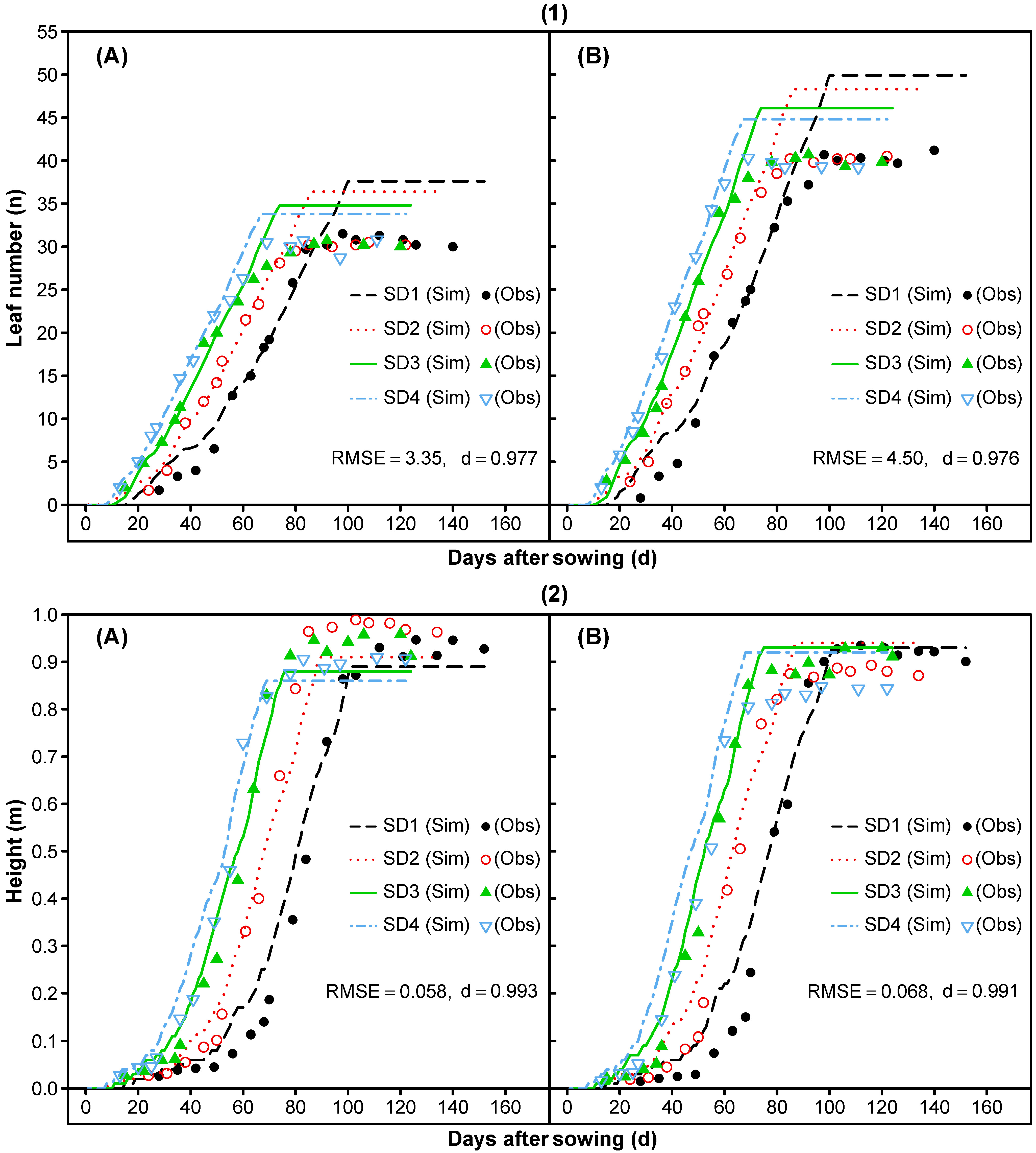
• Parameters that influence the life cycle (threshold values for the cultivar-specific phase duration of different development phases) were changed to predict the correct dates of the first pod, anthesis, and harvest maturity. Then, to ensure an adequate prediction of the leaf number and canopy height and width, the leaf appearance rate, the internode length per node, and the canopy width per node were adjusted by comparing observed and simulated values.
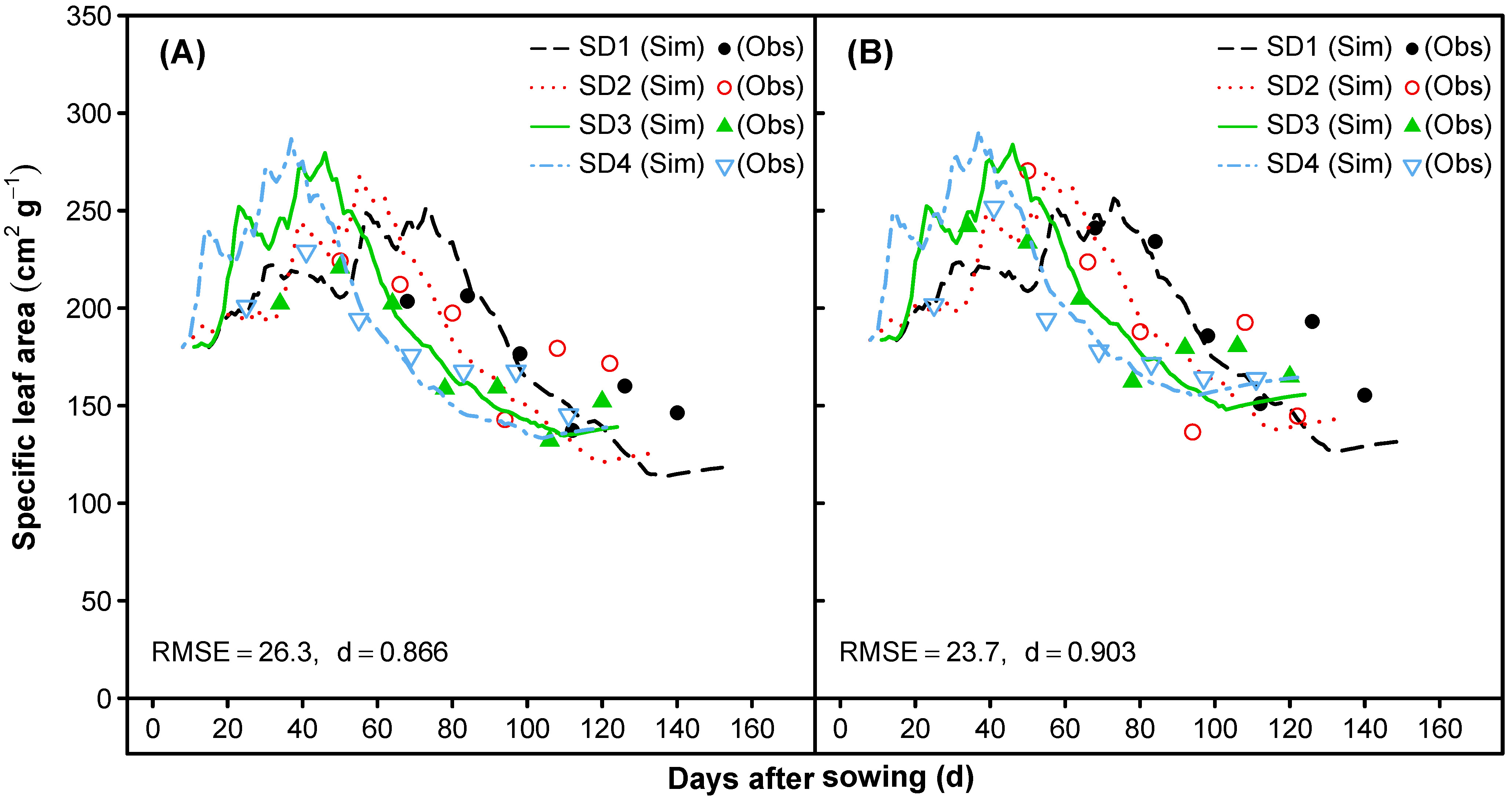
• The next step focused on the parameterization of traits influencing photosynthesis, and consequently, the biomass production during the life cycle. The first target was to match the observed values for the specific leaf area (SLA) over time. Therefore, the default values for the radiation effect on the SLA under saturating irradiance (SLAMIN) and under limiting low light (SLAMAX) were adjusted. Furthermore, we set very minor differences in the cultivar-specific SLA under standard growth conditions (SLAVAR), which is similar to the species-standard SLA in saturating irradiance (SLAREF = SLAMIN). Continuing the improvements of the simulated biomass production over time, the specific leaf weight (SLW) giving the maximum photosynthetic rate (LFMAX) was calibrated and LFMAX was defined based on our own field measurements (not shown). The critical leaf N concentrations for photosynthesis were set in accordance to own data collected in a hydroponic experiment that included different N-concentrations (unpublished).
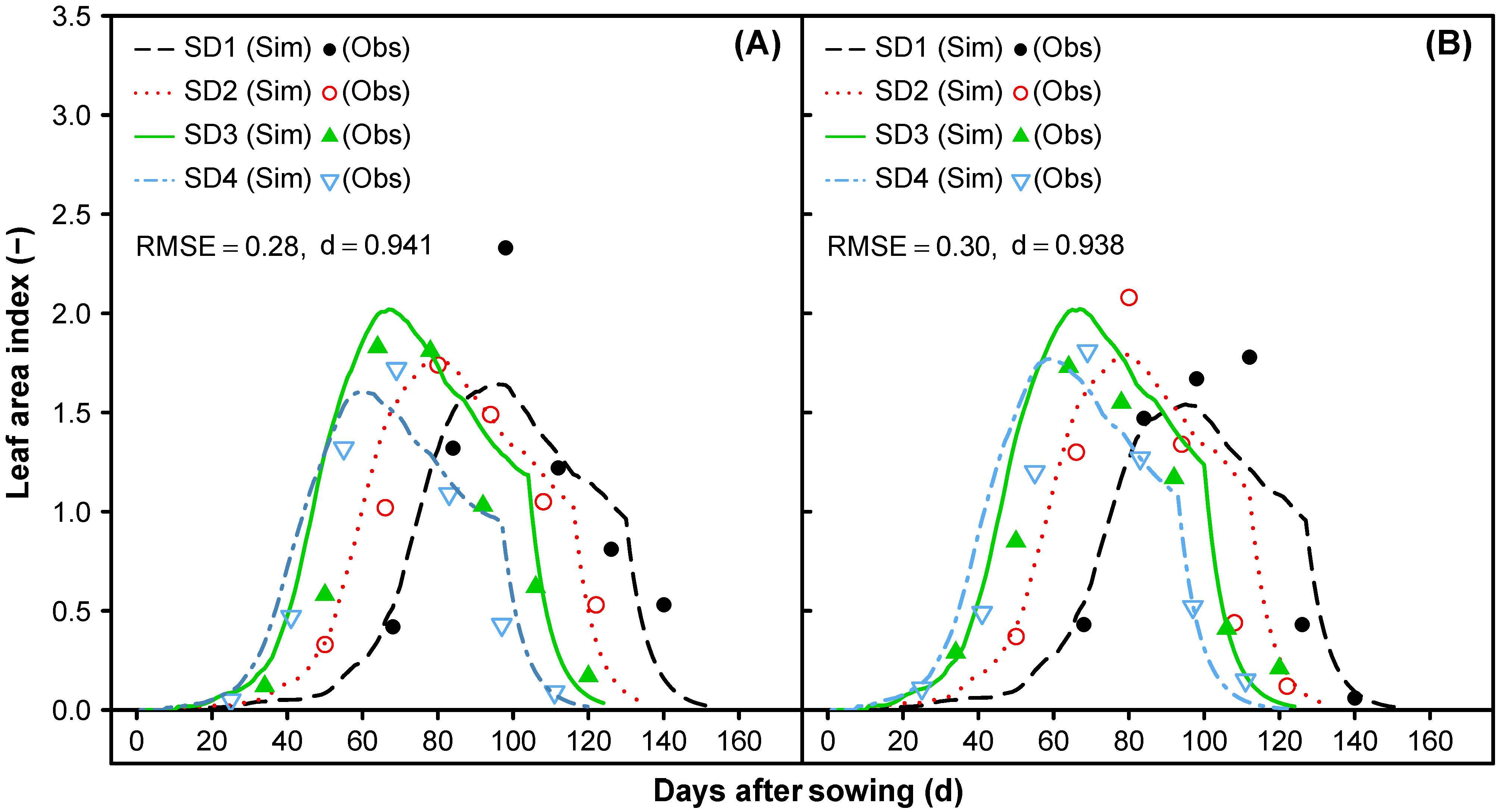
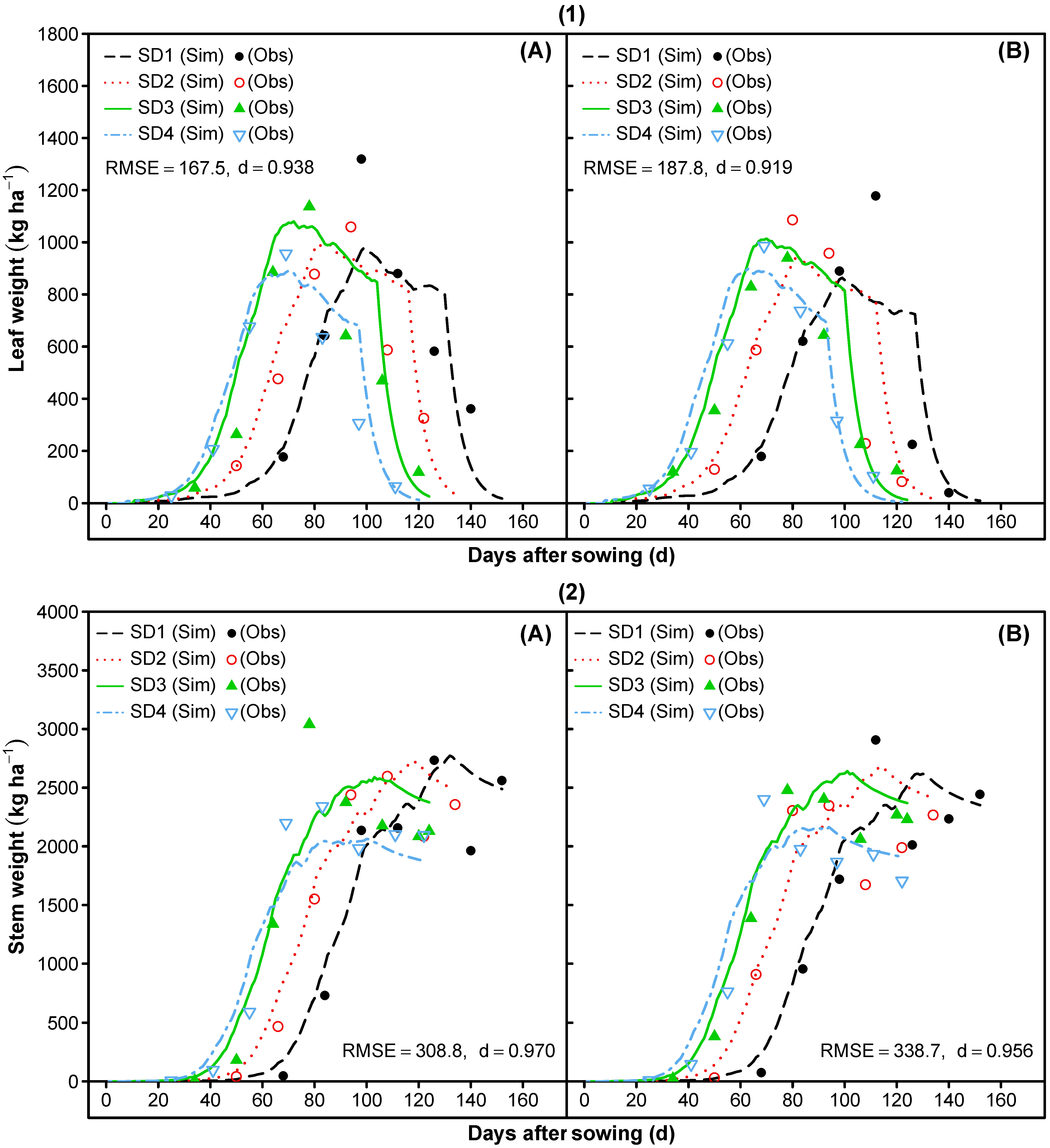
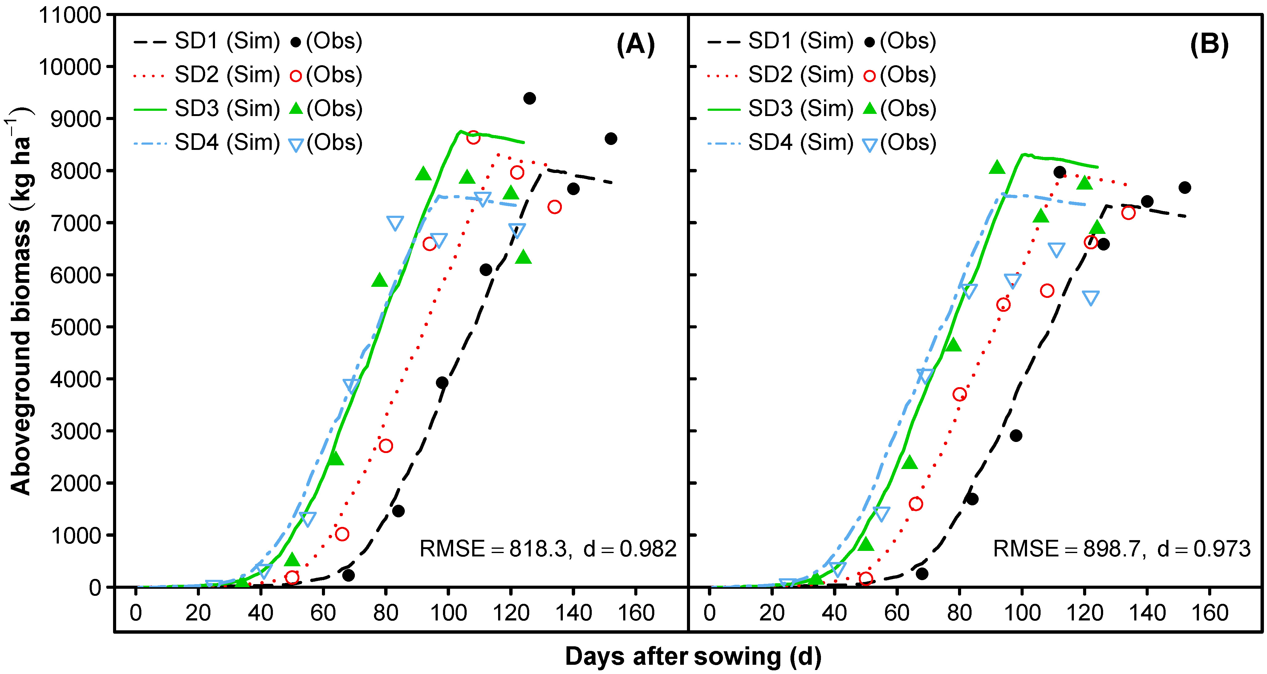
• Time-series comparisons of the predicted and observed dry matter accumulation for leaf, stem, and total aboveground biomass, as well as the leaf area index (LAI), were conducted to parameterize the partitioning functions and to set a final allocation among vegetative tissues. The focus was on the early leaf area development to reach a sufficient leaf area index (LAI), and consequently, a higher photosynthetic performance of the quinoa canopy to adequately predict the dry matter accumulation of the leaf, stem, and aboveground biomass over time.
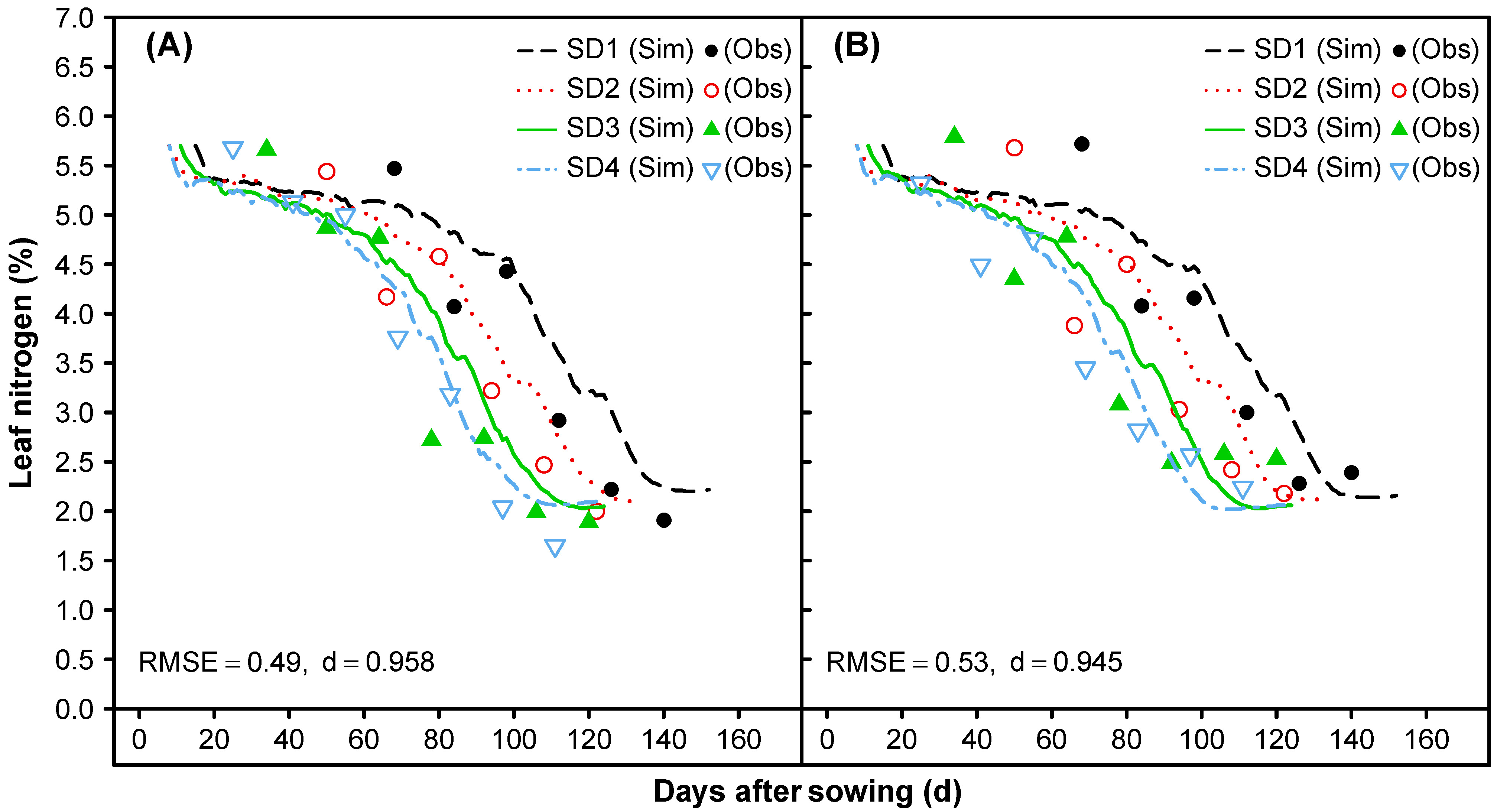
• To match the measured N concentrations of leaves, stems, and shells over time, the maximum mobilization rate (from vegetative tissues) of proteins and carbohydrates during reproductive and vegetative growth was adjusted.
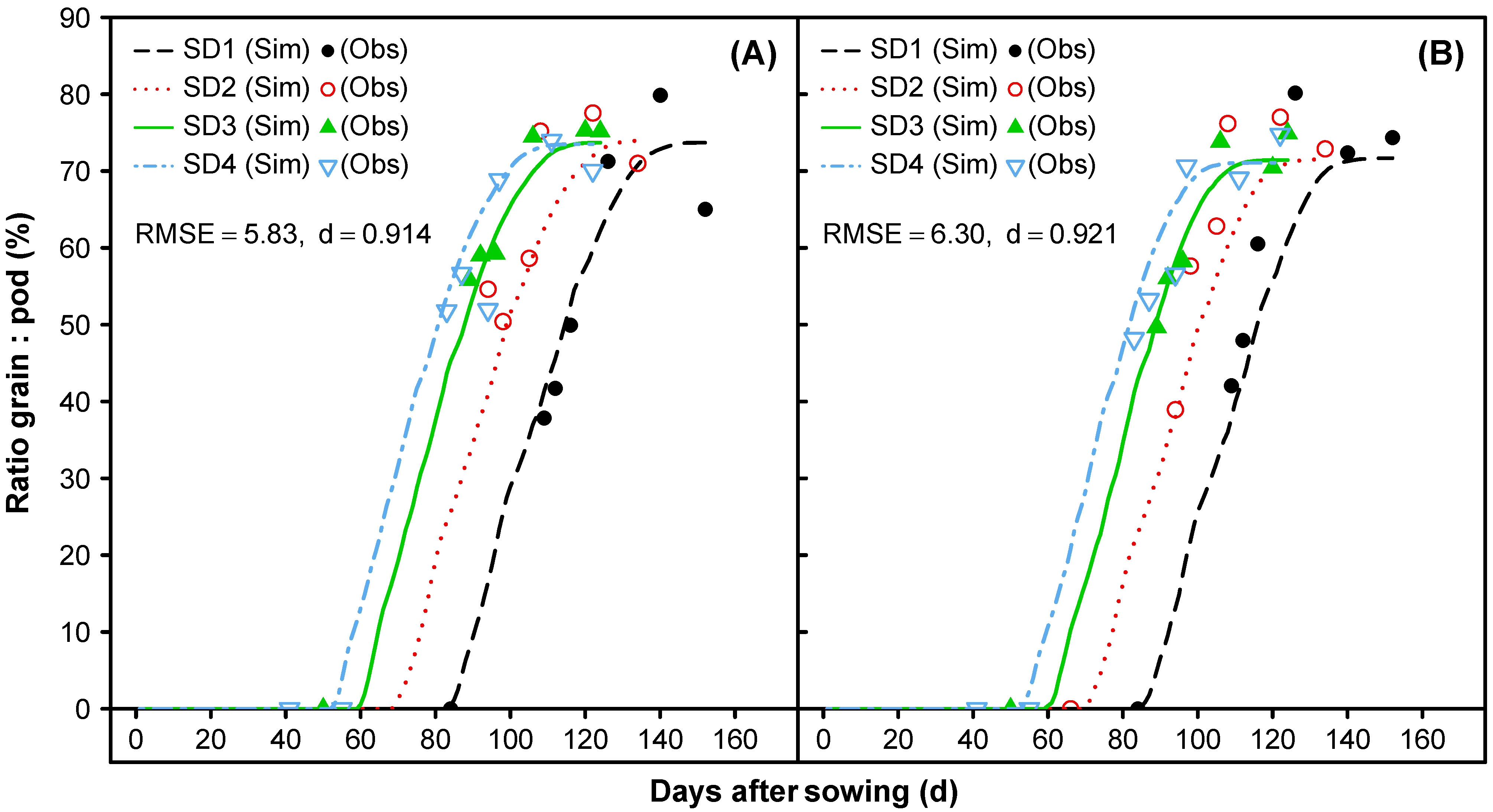
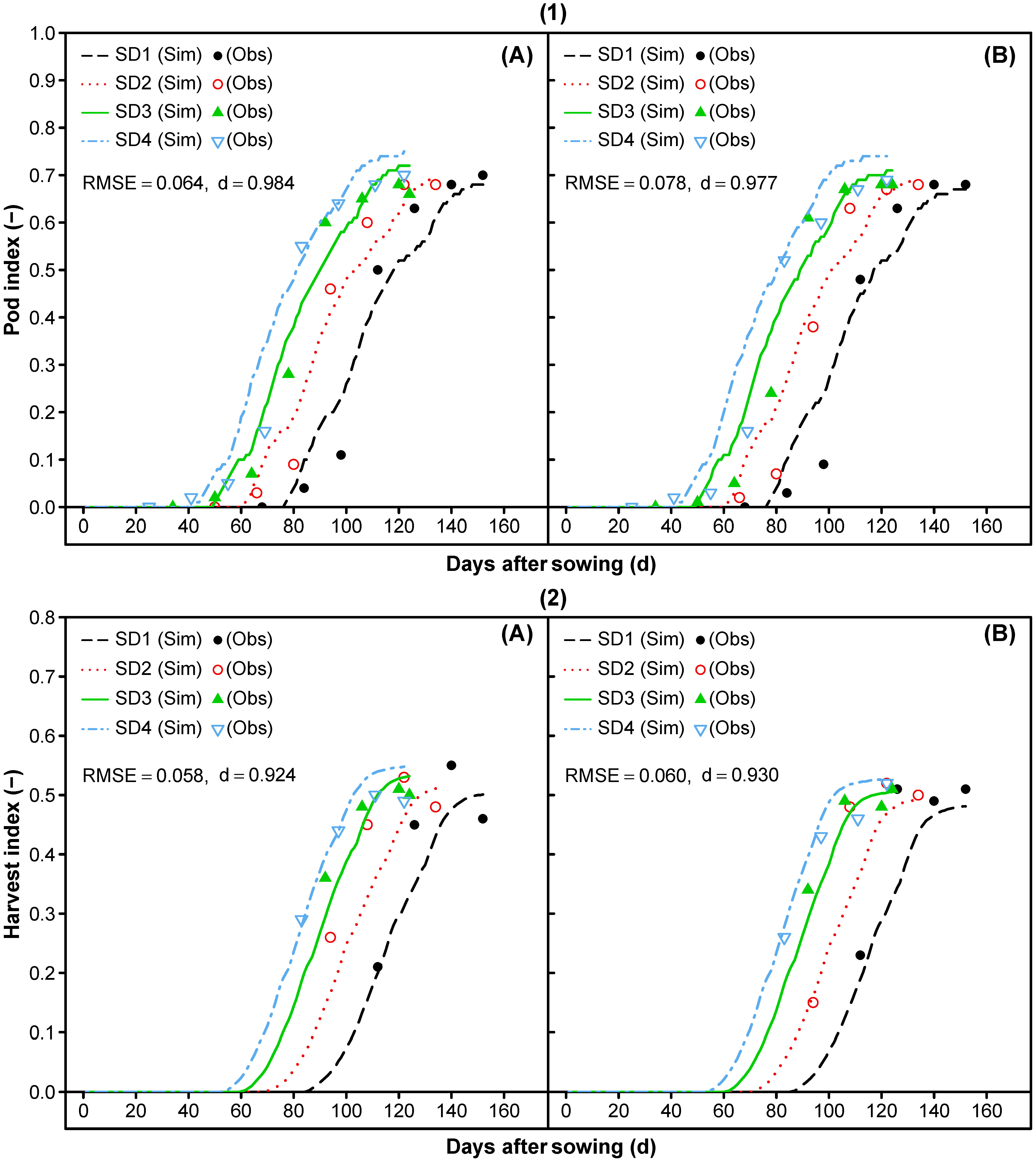
• Re-parameterization of cultivar-specific phase durations was done to match the measured values of the onset and slope of the dry matter accumulation for reproductive tissues. Furthermore, periods for pod addition (PODUR) and seed filling (SFDUR) were shortened and the maximum grain to pod ratio (THRESH) was adjusted to reach an adequate prediction of the pod dry matter, grain dry matter, pod harvest index, grain harvest index, and grain to pod ratio over time.
• Finally, the maximum weight per seed (WTPSD) was set to the lowest value allowed by the model (0.06 g) because the measured values (2.5–3.5 mg) led to source-code-related problems when simulating the reproductive growth (model failed to produce grains). A code change was not attempted because our aim was to be compatible with the default executable of V4.7 DSSAT.

Considerable iterations occurred between the above-mentioned steps using comparisons of measured and simulated growth data (steps 2, 3, 4, 5, and 6 above).

2.6. Model Evaluation Statistics

Simulations with the new quinoa model were evaluated by comparing the simulated and observed time-series and final (harvest) data. The statistical indices were the root mean square error (RMSE) and Willmott agreement index (d-index; [62]). The RMSE gives information about the overall deviation between the simulated and observed values in the unit of the variable with zero indicating a perfect fit, and the d-index shows the conformity for general trends between simulated and observed data. Values can vary between 0 and 1, with a value of 1 indicating perfect agreement between the simulated and observed data.

The RMSE was calculated using the following equation:

$$\mathrm{RMSE}=\sqrt{{\displaystyle \sum }_{\mathrm{i}=1}^{\mathrm{n}}\frac{{({\mathrm{S}}_{\mathrm{i}}-{\mathrm{O}}_{\mathrm{i}})}^2}{\mathrm{n}}},$$

(1)

and the d-index was calculated as follows:

$$\mathrm{d}=1-\frac{{{\displaystyle \sum }}_{\mathrm{i}=1}^{\mathrm{n}}{({\mathrm{O}}_{\mathrm{i}}-{\mathrm{S}}_{\mathrm{i}})}^2}{{{\displaystyle \sum }}_{\mathrm{i}=1}^{\mathrm{n}}(|{\mathrm{S}}_{\mathrm{i}}-\overline{\mathrm{O}}|+|{\mathrm{O}}_{\mathrm{i}}-\overline{\mathrm{O}}|{)}^2},$$

(2)

where n is the number of observations, O_i are the observed values, S_i are the corresponding simulated values, and $\overline{\mathrm{O}}$ is the mean of the observed value for the i^th observation.

3. Results and Discussion

3.1. Model Adaptation

In general, to understand the influence of uncontrollable environmental effects (temperature, soil characteristics, etc.), the usage of growth data that is not affected by water and nitrogen stress is the best way to estimate the model parameters for potential biomass accumulation of a new crop [50]. Using the measured rainfall datasets, the simulation of soil water balance showed no evidence for water stress affecting photosynthesis during the growth cycles of different sowing dates in 2016 (not shown). In contrast, simulation of the nitrogen stress showed significant deficiencies in the nitrogen availability during the growth cycles of all sowing dates in 2016 (not shown). Due to sufficient nitrogen fertilization rates, high soil organic carbon contents (2.8%), and no observed evidence of N-deficiency, the simulated nitrogen stress was not attributed to an inadequate nitrogen supply. The other, more coherent, explanation was the legume typical biotic N-fixation turned off for CROPGRO adaptation on quinoa requirements. This may have disclosed source-code-related model problems regarding the DSSAT soil carbon (C) module, or rather the associated routines used for N mineralization. Therefore, the simulation of the N-balance for the model adaptation and evaluation purposes was turned off in this study under the assumption of an adequate N supply.

3.1.1. Temperature-Dependent Processes

In the CROPGRO model, development and growth processes depend on linear or quadratic temperature functions defined by the cardinal temperatures of each process. Above a certain base temperature (T_b) necessary to start the growth or development process, the relative rate increases with temperature up to an optimal value (T_opt1) and remains the highest until the highest optimum temperature (T_opt2). Temperatures above T_opt2 lead to a decline in the relative development or growth rate up to a ceiling temperature (T_max), where the rate of progress becomes zero.

The germination rate of quinoa was estimated to be equal to zero at temperatures around 3 °C and the optimum temperature was between 30 and 35 °C [63]. In contrast, an evaluation of ten cultivars at temperatures between 2 and 20 °C resulted in T_b estimates of −0.4 to 0.2 °C for the germination rate of quinoa [16].

The base and optimum temperature for the rate of leaf appearance of nine quinoa cultivars was estimated using six temperature regimes in naturally lit growth cabinets [64]. The base temperature ranged from −2–3.8 °C showing a mean value of 1.9 °C, while the optimum temperature ranged from 20.3–23 °C, resulting in a mean value of 22 °C. Similarly, Bois et al. [16] calculated a common base temperature of 1 °C for the rate of leaf appearance (three cultivars) using the results of 13 experiments, while the leaf growth, or rather leaf area expansion, was reported to have a base temperature around 6 °C and an optimum temperature around 22 °C. Following the reported results on the temperature requirements of vegetative development (leaf appearance) and leaf area expansion, we used a base temperature of 1 °C and 6 °C, respectively (

Table 6. Modified cardinal temperatures used in the CROPGRO species file for the development and growth processes of quinoa.

Development or Growth Processes	Description	Cardinal Temperatures (°C)
		Tb 1	Topt1 2	Topt2 3	Tmax 4
Vegetative development	Node expression/germination rate	1.0	22.0	30.0	45.0
Early reproductive development	Flowering to first seed	2.0	24.0	30.0	45.0
Late reproductive development	First seed to maturity	4.0	22.0	30.0	45.0
Light-saturated leaf photosynthesis	LFmax 5 vs. current temperature	2.0	32.0	36.0 8	44.0
Light-saturated leaf photosynthesis	LFmax 5 vs. night temperature	−3.0	15.0	‒ 9	‒ 9
Relative leaf area expansion	Effect on specific leaf area	6.0 6	22.0	‒ 9	‒ 9
Internode expansion	Effect on height and width	9.0 7	19.0	‒ 9	‒ 9
Pod set	Effect on Pod and seed addition	10.0	22.0	26.5	41.0

¹ Base temperature. ² First optimum temperature. ³ Second optimum temperature. ⁴ Maximum temperature. ⁵ Maximum leaf photosynthetic rate. ⁶ Relative rate was 0.46 at T_b. ⁷ Relative rate was 0.45 at T_b. ⁸ Relative rate was 0.80 at T_opt2. ⁹ Relative rate remained high above T_opt1.

). Furthermore, both processes were modified to have the same first optimum temperature of 22 °C.

In comparison to the vegetative development of quinoa, the progress of the early reproductive stage was reported to have a slightly higher base temperature of 1.7 °C [16]. Another evaluation of nine quinoa cultivars resulted in an average base temperature around 2.5 °C (excluding two relatively high values about 5.6 and 4.2 °C), with a corresponding optimum temperature of 19 °C [65]. However, these values were developed during a controlled environment study, which only varied the temperatures but maintained the radiation intensity. Evaluations against the field data, where temperature and radiation were correlated, led to the conclusion that T_opt might be underestimated due to existing interactions between the radiation and high temperatures. Therefore, progress to anthesis was tested under a constant temperature of 24 °C but with different radiation levels. Compared with the optimum temperature developed during the previously mentioned experiment, the time to reach anthesis was similar when combining 24 °C and a high irradiance [65]. Thus, T_b and T_opt1, used for the progress of early reproductive development, was set at 2 °C and 24 °C, respectively (Table 6). Regarding the late reproductive development of quinoa, there is only a small amount of data available on T_b and T_opt. In general, the temperature requirements on quinoa seed filling are very exacting. At 28 °C during seed filling, a decreased seed diameter was observed, and consequently, a strong inhibitory effect of high temperatures during the seed-filling phase was concluded [66,67]. Similar results were reported for quinoa grown in USA, where temperatures exceeding 30–35 °C during anthesis or the seed-filling stage were associated with pollen sterility, a poor seed set, and consequently low yields [68,69]. Following the reported temperature restrictions during anthesis and the grain-filling stage, a T_opt2 of 30 °C was set in the CROPGRO species file for the early and late reproductive development of quinoa. To be consistent, this temperature was also used as the second optimum for vegetative development (Table 6). Since there was no information available on the first optimum temperature of late reproductive development, it was modified according to the value used for the progress of vegetative development (22 °C). The base temperature for late reproductive development was assumed to be slightly higher compared with early reproductive development, but information from the literature was lacking. Starting with 2 °C, we performed stepwise increments of the base temperature to test the parameter sensitivity. The best results were achieved using a base temperature of 4 °C (Table 6), giving reasonable results for all sowing dates (trial 1). As a maximum temperature, above which the rate of progress is zero, 45 °C was selected for all developmental stages of quinoa.

Contrary to the developmental processes, the growth processes of quinoa, such as stem expansion or maximum leaf photosynthetic rate, are stimulated by high temperatures [70,71,72]. Leaf–gas exchange measurements at different leaf temperatures of quinoa, from 10–30 °C, resulted in a first optimum temperature of 30 °C regarding light-saturated leaf photosynthesis. However, the estimated temperature response curve allowed for the assumption of a slightly higher T_opt1 for leaf photosynthesis [73]. Depending on the mean growth temperature, Pearcy et al. [74] observed a similar T_opt1 between 28 and 30 °C when investigating the leaf photosynthesis of Chenopodium album L., a close relative of quinoa. Furthermore, the temperature range resulting in the maximum leaf photosynthetic rate of Chenopodium album L. was found to be very small, showing a second optimum temperature around 36 °C, where the photosynthetic rate was about 80% of the maximum value. Taking the reported literature into account, the values 32 °C (T_opt1) and 36 °C (T_opt 2, relative rate: 0.8) were used for the light-saturated leaf photosynthesis of quinoa (Table 6). The T_b (2 °C) and T_max (44 °C) for leaf photosynthesis were set based on the calibration over all sowing dates (trial 1).

3.1.2. Plant Tissue Composition

Following the method of Penning de Vries and van Laar [75], the CROPGRO model calculates the growth respiration costs and conversion efficiencies of different plant tissues depending on the approximate composition values (protein, carbohydrate-cellulose, lipid, lignin, organic acid, minerals) included in the species file (

Table 7. Maximum values used for the protein concentrations of leaves, stems, roots, and shells and remaining tissue composition used in CROPGRO species file for quinoa (fractions of the total tissue dry weights).

Compound	Plant Tissue	CROPGRO PARAMETER	Quinoa Value	Source of Data 1
Protein	Leaf	PROLFI	0.356	Estimated from own nitrogen data
	Stem	PROSTI	0.200	Estimated from own nitrogen data
	Root	PRORTI	0.092	Soybean model
	Shell (hull)	PROSHI	0.380	Estimated from own nitrogen data
	Seed	SDPROS	0.135	Präger et al. [17]
Carbohydrate	Leaf	PCARLF	0.360	Koziol [77]
	Stem	PCARST	0.511	Carrasco et al. [82]
	Root	PCARRT	0.711	Soybean model
	Shell (hull)	PCARSH	0.330	Calculated/Assumed
	Seed	PCARSD	0.705	Ahamed et al. [76]
Lipid	Leaf	PLIPLF	0.040	Tang et al. [81]
	Stem	PLIPST	0.020	Soybean model
	Root	PLIPRT	0.020	Soybean model
	Shell (hull)	PLIPSH	0.020	Soybean model
	Seed	PLIPSD	0.070	Präger et al. [17]
Lignin	Leaf	PLIGLF	0.080	Schlick [80]
	Stem	PLIGST	0.219	Carrasco et al. [82]
	Root	PLIGRT	0.070	Soybean model
	Shell (hull)	PLIGSH	0.200	Calculated/Assumed
	Seed	PLIGSD	0.025	Ahamed et al. [76]
Organic acid	Leaf	POALF	0.050	Calculated/Assumed
	Stem	POAST	0.025	Calculated/Assumed
	Root	POART	0.050	Soybean model
	Shell (hull)	POASH	0.040	Soybean model
	Seed	POASD	0.040	Calculated/Assumed
Minerals	Leaf	PMINLF	0.114	Bhargava et al. [79]
	Stem	PMINST	0.025	Calculated/Assumed
	Root	PMINRT	0.057	Soybean model
	Shell (hull)	PMINSH	0.030	Soybean model
	Seed	PMINSD	0.025	Ahmed et al. [76]

¹ Baseline for setting the tissue compositions of the new quinoa model.

). Furthermore, the CROPGRO species file includes information on the initial (maximum), growth (normal), and final (minimum) protein concentrations of the leaves, stems, roots, and shells. Composition values of the seed proteins and seed lipids used in species file serve as reference values, which can be overwritten by the specifications included within the cultivar file (

Table 8. Genetic coefficients of quinoa (CROPGRO cultivar file) for the cultivars Zeno and Jessie after adaptation.

CROPGRO Parameter	Description	Quinoa Cultivar
		Zeno	Jessie
PP-SEN	Slope of the relative response of development vs. photoperiod (1 h−1)	0.008	0.008
EM-FL	Time between plant emergence and flower appearance (PD 1)	11.200	11.200
FL-SH	Time between first flower and first pod (PD)	2.900	3.000
FL-SD	Time between first flower and first seed (PD)	8.600	9.100
SD-PM	Time between first seed and physiological maturity (PD)	34.400	30.900
LFMAX	Maximum leaf photosynthetic rate under 30 °C, 350 µL L−1 CO2, and high light (mg CO2 m−2 s−1)	1.730	1.700
SLAVR	Specific leaf area of a cultivar under standard growth conditions (cm2 g−1)	250.000	255.000
SIZLF	Maximum size of full leaf (cm2)	7.000	6.500
XFRT	Maximum fraction of daily growth that is partitioned to seeds + shells	1.000	0.980
WTPSD	Maximum weight per seed (g)	0.060	0.060
SFDUR	Seed filling duration for pod cohort under standard growth conditions (PD)	22.000	22.500
PODUR	Duration of pod addition under optimal conditions (PD)	16.000	15.000
THRSH	Maximum grain to pod ratio at maturity (%)	75.500	74.500
SDPRO	Fraction protein in seeds (g(protein) g(seed)−1)	0.125	0.150
SDLIP	Fraction oil in seeds (g(oil) g(seed)−1)	0.055	0.070

¹ Photothermal days.

). The maximum protein contents and remaining composition values for each plant tissue must be equal to 1.0. Except for the protein values for leaves, stems, and shells, which were set on the basis of nitrogen values measured during the 2016 growth period (trial 1), composition values for different plant tissues were set within the range of literature-reported composition values for quinoa. If the literature information was lacking, values from the soybean model were taken, or values were assumed by deducting the sum of particular values from 1.0 [26]. The mean values of quinoa seeds for different cultivars were between 12–16% protein [17], 61–74% carbohydrate [76], 5.5–7.5% crude fat [17], and 2–3% crude fiber [76]. Regarding the mineral content of quinoa seed, broad ranges of 1.4–7.6% [76] or 2.0–6.1% [77] were reported in the literature.

The protein concentration of leaves was estimated to have an initial value of 35.6% (5.7% N), a typical value during growth of 28.5% (4.6% N), and a minimum value of 9.2% (1.5% N). Carbohydrates make up 32–36% of the total dry matter of quinoa leaves [77]. Furthermore, quinoa leaves can accumulate comparatively high concentrations of minerals [78], showing a range of 4.6–26.9% [79]. The crude fiber concentration, which served as an estimate for leaf lignin in the current quinoa model, varies between 8.0 [80] and 13.9% [77]. Lipids are minor constituents of quinoa leaves, showing a mean proportion of 4% with almost no variation among cultivars [81].

Based on our data on N concentrations during the growing period in 2016 (trial 1), the maximum value for the protein concentration of stems was set to 20% (3.2% N), while typical and minimum protein concentrations were around 10% (1.6% N) and 3% (0.5% N), respectively, in stem dry matter. Furthermore, quinoa accumulates high amounts of xylan (15.4–17.9%) and glucan (35.7–37.9) [82] in the stem. Based on these values, the composition value for stem carbohydrate (includes cellulose) concentration was set to 51.1%. As a second major stem component, lignin was reported to range between 21.9 and 23% [82].

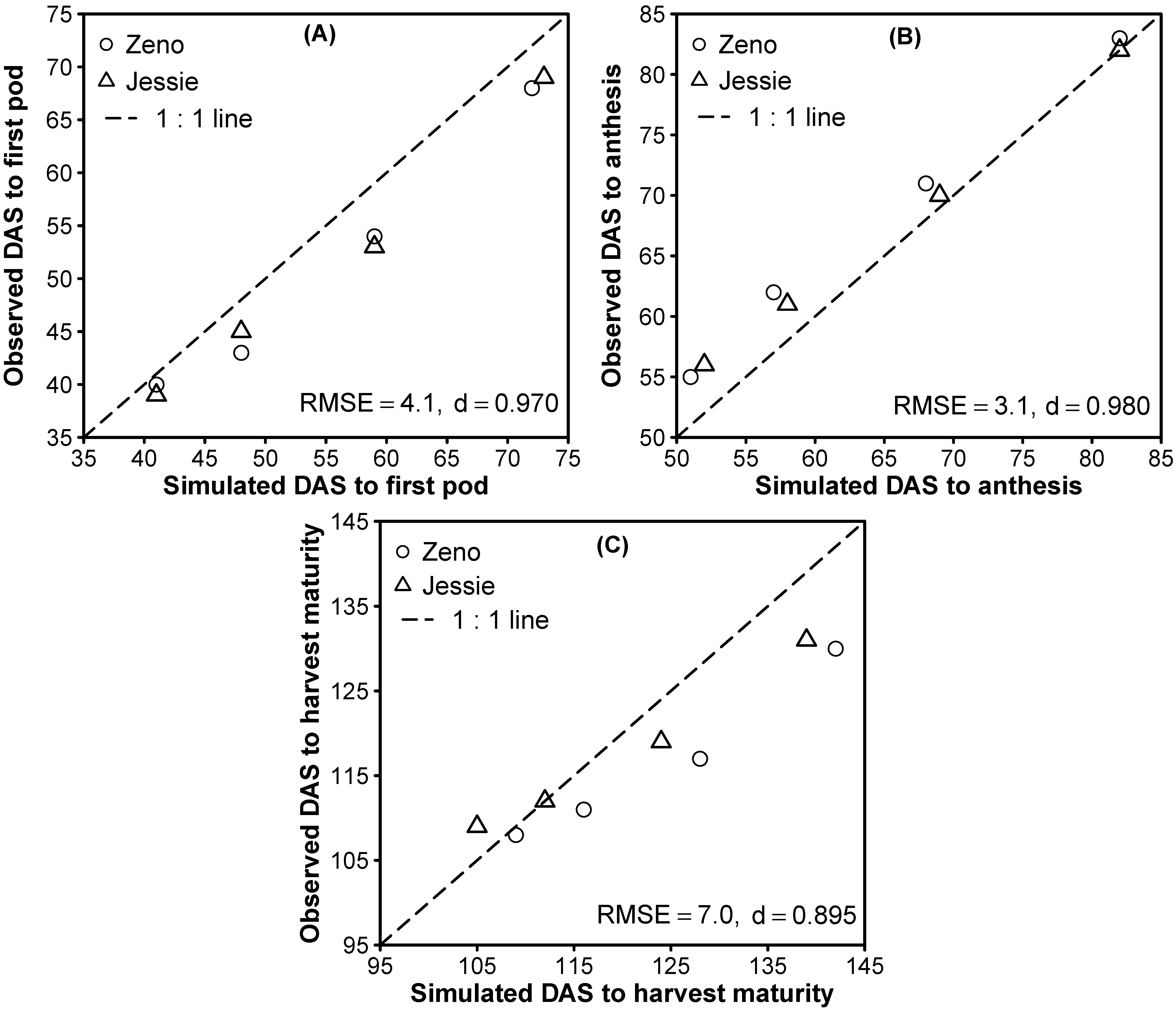
3.1.3. Phase Durations and Phenology

Most original quinoa landraces can be categorized as facultative short-day plants, flowering under any photoperiod, but reproductive development continues only under a short-day photoperiod (<12 h) [56]. However, during the adaptation process of quinoa to northern latitudes, ecotypes originating from the coastal regions of southern Chile were found to show a high level of photoperiodic insensitivity during the reproductive phase. Consequently, these ecotypes were used for the further breeding of European cultivars [56]. Therefore, quinoa was modeled as a photoperiodic insensitive plant in the current study, assuming a critical photoperiod of 14.35 h, below which, progress to anthesis and reproductive development was the most rapid. Additionally, we used an apparent sensitivity (PP-SEN) of 0.008 for both cultivars that defined the slope of the relative decrease (1 h⁻¹) in the rate of progress for photoperiods longer than the critical threshold assumed (Table 8). A PP-SEN value of 0.008 ensured nearly complete daylength-insensitivity.

In quinoa, pods (inflorescences) appear before anthesis and seed growth starts very soon after anthesis. Therefore, we followed the procedure described by Singh et al. [26] and integrated the real anthesis date in the CROPGRO model only as a dummy variable while creating a false flower, with the aim of predicting the beginning of the seed set (R5) in the CROPGRO model corresponding to the observed quinoa anthesis.

Simulation of the first pod date, anthesis date, and harvest maturity date was calibrated using comparisons with observed data. Four CROPGRO cultivar parameters defining the phase durations of the time between plant emergence and flower appearance (EM-FL), time between first flower and first pod (FL-SH), time between first flower and first seed (FL-SD), and time between first seed and physiological maturity (SD-PM) were relevant parameters to reach an adequate prediction of the quinoa life cycle. The first pod date required the sum of EM-FL and FL-SH. To create a better partitioning transition to stem during the later life cycle, we set EM-FL to the maximum possible value (11.2 photothermal days (PD) for both cultivars), while minimizing FL-SH (Table 8). Subsequently, targeting a reasonable prediction of the “real” anthesis date, FL-SD was set to 8.6 and 9.1 PD for cv. Zeno and cv. Jessie, respectively (Table 8). The time between first seed and physiological maturity was set to 34.4 PD (cv. Zeno) and 30.9 PD (cv. Jessie) to match the simulated and observed values of harvest maturity dates. Including both cultivars and the four sowing dates in 2016 (Trial 1) overall RMSEs for the prediction of first pod, anthesis (beginning seed in the CROPGRO model), and harvest maturity dates were 4.1, 3.1, and 7.0 days, respectively (Figure 1).

The CROPGRO model predicts crop height and width as a function of the increase in main stem node number and corresponding internode length and canopy width. Targeting a correct initialization of the node formation or leaf appearance for both cultivars, the time between planting and emergence (PL-EM), as well as the time required from emergence to first true leaf (EM-V1), was adapted to 3.2 and 2 thermal days, respectively (

Table 9. Parameters as defined in the CROPGRO ecotype file for quinoa after adaptation.

CROPGRO Parameter	Description	Quinoa Ecotype
		1 (cv. Zeno)	2 (cv. Jessie)
PL-EM	Time between planting and emergence (thermal days)	3.2	3.2
EM-V1	Time required from emergence to first true leaf (thermal days)	2.0	2.0
FL-VS	Time from first flower to last leaf on main stem (PD 1)	20.0	20.0
TRIFL	Rate of leaf appearance on the main stem (leaves per thermal day)	0.9	1.2
RWDTH	Relative width of this ecotype in comparison to the standard width per node defined in the species file	1.0	0.8
RHGHT	Relative height of this ecotype in comparison to the standard height per node defined in the species file	1.0	0.8

¹ Photothermal days.

). The simulation of leaf number was increased by setting the main stem leaf appearance rate (TRIFL) to 0.9 (cv. Zeno) and 1.2 (cv. Jessie) leaves per thermal day. These values resulted in an accurate prediction of the observed leaf tip number over time, showing a d-index of 0.977 and 0.976 for cv. Zeno and cv. Jessie, respectively (Figure 2). Since we observed a leaf tip number on the main stem instead of the CROPGRO standard (number of fully developed leaves), the specified TRIFL values were comparatively higher than the soybean value of 0.32; however, we believe quinoa has a faster leaf appearance rate than soybean. In addition, the CROPGRO model uses the fully-expanded main stem leaf number to simulate the canopy height, which in turn has a considerable impact on the light interception, and consequently, canopy photosynthesis [83]. Because the leaf tip appearance ends several plastochrons prior to the full expansion of leaves (and internode extension), a modest compromise on the timing of the end of leaf appearance was made to achieve the canopy height. Hence, the coefficient that defines the termination of continued leaf formation on the main stem (FL-VS) after the false flower date was set to 20 PD, slightly higher than the leaf number data suggested. This gave a tolerable overprediction of the final leaf number, but a reasonable estimation of canopy height (Figure 2). Nevertheless, across all sowing dates, the RMSEs for the simulated main stem leaf number showed acceptable values of 3.5 and 4.5 for cv. Zeno and cv. Jessie, respectively. Besides the improvements for the simulations of leaf appearance and final leaf number, further height parameters were modified to reach an adequate canopy light interception over time. The temperature sensitivity of internode elongation was calibrated to have a T_b of 9 °C, giving 0.45 of the normal internode lengths, and a T_opt1 of 19 °C, above which, normal (1.0) internode length can be reached (Table 6). Furthermore, the lookup table defining the maximum potential internode length at corresponding nodes above the cotyledon node was modified. According to observed data (Figure 2), internodes during the early vegetative stage (until node number 10) were modeled to be shorter with successive internodes showing only slight increments in length. The length of the internodes later in the life cycle were longer, showing a more rapid, successive increase in elongation until about half of the final node number was expressed (

Table 10. Internode length and canopy width as a function of the main stem node number used in the CROPGRO species file for quinoa.

Height or Width (m Internode−1)	Node Number (Leaf Number)
	0	1	4	6	8	10	14	18	25	50
Internode length	0.010	0.013	0.013	0.016	0.019	0.022	0.029	0.036	0.042	0.028
Canopy width	0.010	0.010	0.011	0.012	0.013	0.013	0.012	0.011	0.011	0.010

). These specifications were made based on the growth analyses of cv. Zeno, which served as a reference within the species file. Regarding cv. Jessie, the parameter for the relative height of an ecotype in comparison to the standard height per node defined in the species file (RHGHT) was adjusted to 0.8 to take the larger node number of this ecotype into account (Table 9). Generally, the maximum height of both quinoa cultivars sown on four sowing dates was reached at the beginning of seed development, with mean values between 0.90 m and 0.96 m for cv. Zeno, as well as between 0.84 and 0.91 m for cv. Jessie. The simulated canopy height showed a good fit across the four sowing dates with RMSEs of 0.058 and 0.068 m and d-indexes of 0.993 and 0.991 for cv. Zeno and cv. Jessie, respectively (Figure 2).

3.1.4. Specific Leaf Area and Photosynthesis

To predict the response of the specific leaf area (SLA) to solar radiation, an upper (thinnest leaves, under low radiation) and lower limit (thickest leaves, under high radiation) of the SLA was defined in the species file. While keeping the minimum possible SLA (SLAMIN) as the default, the possible maximum SLA (SLAMAX) was decreased to 760 cm² g⁻¹ (

Table 11. Modified parameters used in CROPGRO species file for development and growth processes of quinoa.

Development or Growth Processes	CROPGRO Parameter	Description	Quinoa Value
Photosynthesis	SLWREF	Specific leaf weight at which LFMAX is defined (g cm−2)	0.0034
	LNREF	Leaf N concentration (%) at which LFMAX is defined	4.5
Nitrogen or carbon mining	NMOBMX	Maximum fraction of protein pool (from vegetative tissues) mobilized per day during reproductive growth	0.125
	NVSMOB	Relative protein mobilization during vegetative growth (ratio on NMOBMX)	0.65
Vegetative partitioning	PORPT	Gram (g) of stem mass abscised per g of leaf	0.06
	FRSTMF	Fraction of vegetative dry matter growth allocated to the stem at the final stage	0.65
	FRLFF	Fraction of vegetative dry matter growth allocated to leaves at the final stage	0.20
Leaf growth	SLAREF	The specific leaf area (cm2 g−1) of the reference cultivar at peak vegetative phase	250.0
	SIZREF	Leaf area (cm2) for the leaf at the fifth node position	30.0
	SLAMAX	Maximum specific leaf area (cm2 g−1) under low light	760.0
	SLAMIN	Minimum specific leaf area (cm2 g−1) under saturating light	250.0
Leaf senescence	SENRT2	Rate of leaf abscision after physiological maturity (fraction day−1)	0.16
	FREEZ1	Temperature (°C) that kills leaves, but stems, pods, and seeds remain alive and seeds can grow on mobilized reserves	−5.50
	FREEZ2	Temperature (°C) below which development and crop growth simulation stops	−8.50

). Following the observations for cv. Zeno during the peak vegetative phase, the reference SLA (SLAREF, same as SLAMIN) contained in the species file was set to 250 cm² g⁻¹. Consequently, the cultivar-dependent SLA under standard growth conditions (SLAVAR) for cv. Zeno was set to the same value as SLAREF (Table 8). Considering the general observation of its thinner leaves, SLAVAR for cv. Jessie was set slightly higher to 255 cm g⁻¹. The cultivar-dependent SLA specified for cv. Zeno and cv. Jessie was consistent with the literature, which reports values between 144–277 cm² g⁻¹ [84]. Averaged across the four sowing dates in 2016, the observed mean SLA of the growing period was 179.5 and 192.7 cm² g⁻¹, for cv. Jessie and cv. Zeno, respectively. Simulated values were very close, showing a mean SLA of 180.1 (cv. Zeno) and 190.9 cm² g⁻¹ (cv. Jessie), and a corresponding d-index of 0.87 and 0.90, for cv. Zeno and cv. Jessie, respectively (Figure 3).

To model the productivity of the quinoa cultivars correctly, the maximum leaf photosynthetic rate (LFMAX, Table 8) was increased based on the field measurements, which were consistent with the literature [71,84]. Values were set to 39.3 µmol CO₂ m⁻² s⁻¹ (1.73 mg CO₂ m⁻² s⁻¹) and 38.6 µmol CO₂ m⁻² s⁻¹ (1.70 mg CO₂ m⁻² s⁻¹) for cv. Zeno and cv. Jessie, respectively.

A sufficient nitrogen supply was reported to be essential for maintaining the LFMAX of different quinoa cultivars [84]. Following the results of the leaf N concentrations found in leaves, used for measuring the maximum photosynthetic rate in the field, the leaf nitrogen concentration (LNREF) giving the maximum photosynthetic rate in the CROPGRO model was set to 4.5% (Table 11). Consequently, the quadratic leaf photosynthesis response function to the leaf N concentration (FNPGN) was also modified. While setting the N concentration for the maximum photosynthesis equal to the value specified for LNREF (4.5%), the minimum leaf nitrogen concentration, giving zero photosynthesis, was decreased to 1.0%. Both values were consistent with previous results derived from a hydroponic trial, which tested the influence of various nitrogen concentrations on maximum photosynthetic rate (not published).

Additionally, the CROPGRO model allows for the relative effect of the minimum night temperature on the next day’s photosynthesis. According to the reported cold tolerance of quinoa [16,85], a low sensitivity against night temperatures was assumed. Hence, the function was calibrated to a T_b of −3 °C (next day’s photosynthetic rate equal to zero) and an asymptotic value of 15 °C without producing limits on the next day’s photosynthesis (Table 6). By comparison, the values for faba bean, another cold-tolerant species, were set to −2 and 14 °C, respectively [50]. Allowing the model to simulate a higher canopy photosynthesis, the specific leaf weight (SLWREF) at which LFMAX was defined was finally reduced to 0.0034 g cm⁻² (Table 11) based on the optimization against the biomass data.

3.1.5. Leaf Area Index and Vegetative Partitioning

The leaf area index (LAI) is simulated based on the SLA and leaf weight. Since dry matter partitioning into leaves was initially insufficient (with soybean parameters), the instantaneous partitioning among leaf, stem, and root tissues as a function of the vegetative development stage (node number) was modified (

Table 12. Relative dry matter partitioning among vegetative tissues (leaves, stem, roots) as a function of the main stem node number used in the CROPGRO species file for quinoa.

Relative Dry Matter Partitioning	Node Number (XLEAF)
	0	3	7	11	16	25	37	40
Leaf (YLEAF)	0.41	0.41	0.41	0.41	0.39	0.33	0.30	0.30
Stem (YSTEM)	0.09	0.13	0.20	0.28	0.35	0.48	0.49	0.49
Root	0.50	0.46	0.39	0.31	0.26	0.19	0.21	0.21

). This was caused by having much faster leaf appearance rates for quinoa; therefore, the soybean-default partitioning function against the leaf number progressed too rapidly toward less leaves and more stem. Thus, the period for partitioning a higher fraction assimilates to the leaves was extended compared with soybean (initial default). Consequently, the period for rapid stem growth, until the addition and growth of pods and seeds became dominant, was delayed and extended. Observations showed that rapid stem growth started just before reaching the peak in LAI or leaf weight observed around anthesis (Figure 4 and Figure 5). Moreover, stem growth reached a plateau close to the end of anthesis, showing no further dry weight increase. To account for this, the node numbers (XLEAF) corresponding to particular partitioning fractions of leaves and stem were shifted to partition larger dry matter fractions into leaves until node number 16 (Table 12). Then, the relative dry matter fractions partitioned into leaves and stem (YLEAF, YSTEM) were slightly adjusted based on optimization against the biomass data.

For improving the simulated early leaf area increase, the leaf area for the fifth node position (SIZREF, Table 11) and maximum size of full leaf (SIZLF, Table 8) were adjusted. Based on the measured data during early vegetative development, SIZREF was set to 30 cm². Since the final leaf number was intentionally overpredicted for both cultivars (Figure 2), we had to calibrate values for the maximum single leaf area, resulting in 7.0 cm² (cv. Zeno) and 6.5 cm² (cv. Jessie).

Simulations of the stem weight over time were further improved by decreasing the parameter defining the ratio of petiole (stem) mass abscised per leaf mass abscised (PORPT) to 0.06 (Table 11). Quinoa does not abscise significant petiole mass, whereas soybean does. Since the CROPGRO model includes petiole mass in the stem mass, reducing PORPT resulted in an increased simulated stem weight during the life cycle.

Using the model modifications discussed above, the LAI, leaf weight, and stem weight of both cultivars were adequately simulated across all sowing dates in 2016. The simulated leaf area index was underpredicted at the peak phase for the first sowing date, while the simulated LAI for late sowing dates started too early, resulting in a slight overprediction before the peak phase (Figure 4). However, averaged over all sowing dates, the simulated mean LAI during the growing period for both cultivars was very close to the observed value, with a simulated mean for cv. Zeno of 1.02 (observed: 0.93) and an RMSE of 0.28, while the simulated mean for cv. Jessie was slightly lower with 0.99 (observed: 0.89) and an RMSE of 0.30. Corresponding d-indices were 0.941 and 0.938, for cv. Zeno and cv. Jessie, respectively.

The simulated leaf weights for both cultivars showed a consistent, slight underprediction for the peak phase (Figure 5). The average RMSE was 167.5 kg ha⁻¹ and 187.8 kg ha⁻¹ for cv. Zeno and cv. Jessie, respectively. The corresponding d-indices were 0.938 (cv. Zeno) and 0.919 (cv. Jessie). The stem weight simulations were even more accurate with average RMSE values ranging from 308.8 kg ha⁻¹ (cv. Zeno, d = 0.970) to 338.7 kg ha⁻¹ (cv. Jessie, d = 0.956).

3.1.6. Leaf Senescence and Nitrogen Mobilization

The leaf senescence factor giving the potential loss of leaves per day after physiological maturity (SENRT2) was calibrated to 0.16 (Table 11). Factors other than crop age considered by the CROPGRO model to cause leaf senescence are drought stress and remobilization of nitrogen (protein) and carbohydrates. However, reproductive growth (seed filling), and consequently yield prediction, is also highly influenced by the potentially mobilizable protein amounts from vegetative tissues (leaves, stems, roots) until physiological maturity. To adequately predict the time course for nitrogen concentrations of vegetative tissues, the daily maximum protein fraction that is mobilizable from the vegetative tissues during reproductive growth (NMOBMX) and the relative intensity of NMOBMX during the vegetative phase (NVSMOB, is a ratio) were modified (Table 11). Based on an optimization against the measured nitrogen concentrations of the leaves, stems, and shells, the values were set to 0.125 (NMOBMX) and 0.65 (NVSMOB). The described changes resulted in reasonable predictions of the leaf nitrogen concentrations (Figure 6). The average RMSEs were 0.49% and 0.53% for cv. Zeno (d = 0.958) and cv. Jessie (d = 0.945), respectively. Stem and shell N concentrations were also well predicted (data not shown). The usage of modified values for NMOBMX and NVSMOB also caused a more rapid decrease in the LAI and leaf weight, which was consistent with the observed data, as shown in the final simulations (Figure 4 and Figure 5). Finally, the CROPGRO species file includes sub-lethal (FREEZ1) and lethal (FREEZ2) thresholds for low temperatures (Table 11). Taking the range of −5 to −6 °C [16] reported for freezing temperatures of quinoa leaves into account, FREEZ1 was set to −5.5 °C, while FREEZ2 was assumed to be −8.5 °C.

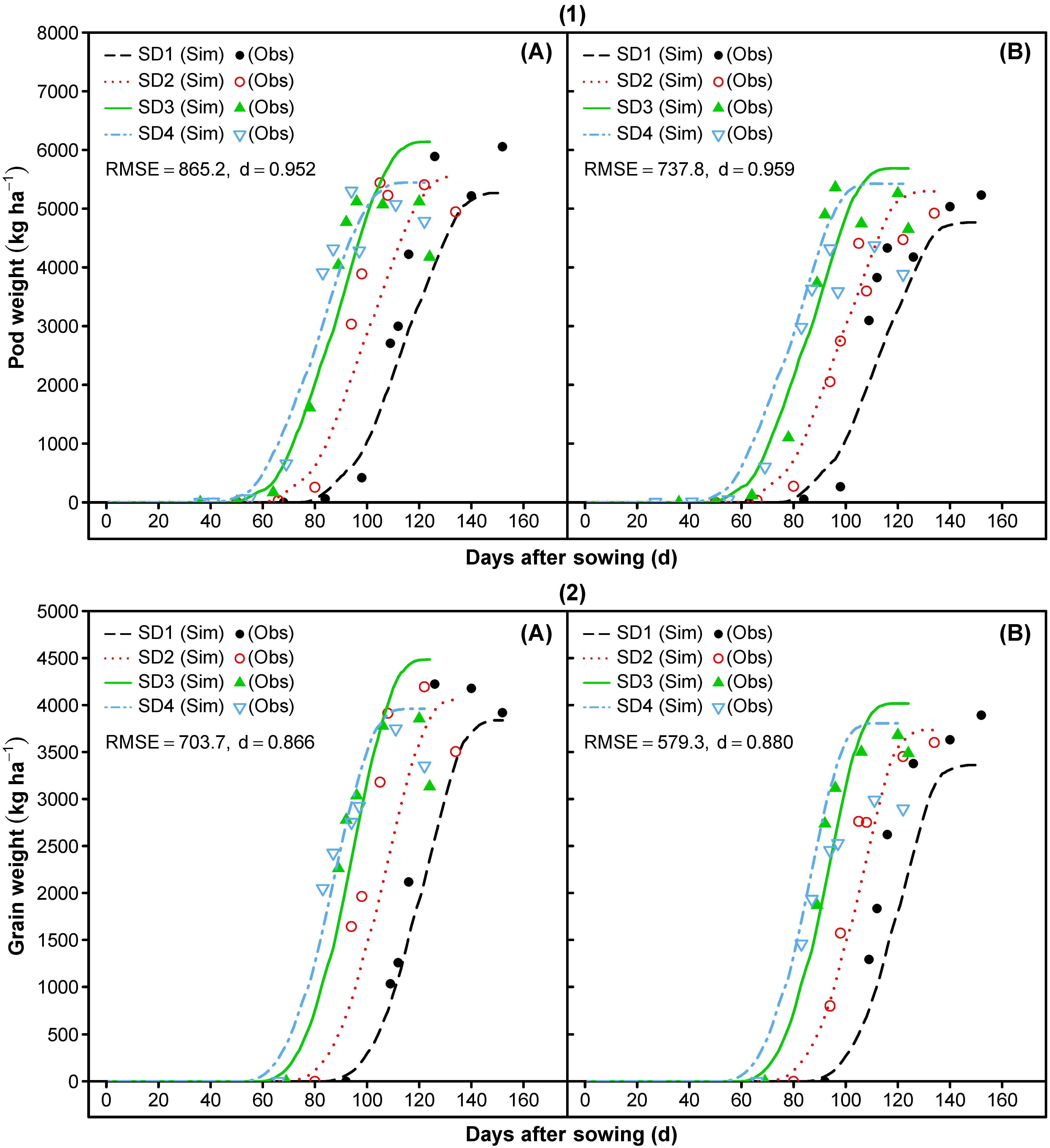
3.1.7. Reproductive Partitioning

The parameters affecting the partitioning among reproductive parts (pod weight and grain weight) were mainly calibrated by comparing the simulated relative ratios of pod harvest index, grain harvest index, and grain to pod ratio with the observed (Figure 7 and Figure 8). Since these ratios are not biased by randomly-taken small biomass samples, this can be considered a reliable method of calibration [50]. Due to the absence of available literature on cardinal temperatures regarding pod addition, these temperatures were initially optimized using comparisons of observed and simulated pod indexes for both cultivars and all sowing dates. The resulting temperatures were 10 (T_b), 22 (T_opt1), 26.5 (T_opt2), and 41 °C (T_max) (Table 6). Moreover, the duration of the pod addition under optimal conditions (PODUR) was calibrated based on cultivar-specific comparisons of observed and simulated values for the pod harvest index and pod weight at different sowing dates. The resulting PODUR was 16 and 15 photothermal days for cv. Zeno and cv. Jessie, respectively (Table 8). In order to reach adequate predictions for the grain harvest index, grain to pod ratio, and grain weight, we finally calibrated the values for the maximum fraction of the daily growth that was partitioned to seed (XFRT), the seed filling duration under standard growth conditions (SFDUR), and the maximum grain to pod ratio at harvest maturity (THRESH) included in the cultivar file (Table 8). Furthermore, the fractions of protein (SDPRO) and oil (SDLIP) contained in the seeds were set according to the literature values reported for cv. Zeno and cv. Jessie ([17], Table 8).

Using these calibrations, the pod harvest index and pod weight were reasonably well simulated. The pod harvest index of both cultivars and all sowing dates was slightly overpredicted in the beginning, while the final values showed a high accuracy (Figure 8). RMSEs of 0.064 and 0.078, with corresponding d-indices of 0.984 and 0.977, were found for cv. Zeno and cv. Jessie, respectively. In contrast, the simulations for the (final) pod weight of both cultivars showed more variation in accuracy when comparing different sowing dates (Figure 9). However, the slopes of pod weight over time were predicted very well for all sowing dates (particularly the onset including a slight early lag), resulting in d-indices of 0.952 (cv. Zeno) and 0.959 (cv. Jessie).

Grain to pod ratio (Figure 7) and grain harvest index (Figure 8) were simulated with high accuracy for all sowing dates and both cultivars. Predictions of the grain to pod ratio showed RMSE values of 5.83% (cv. Zeno, d = 0.914) and 6.30% (cv. Jessie, d = 0.921). Similarly, the grain harvest index showed RMSEs of 0.058 and 0.060 for cv. Zeno (d = 0.924) and cv. Jessie (d = 0.930), respectively. Simulations of the grain weight resulted in sowing-date-dependent accuracies for the final values, while the slopes and onset of grain growth was predicted very well in general for cv. Zeno (RMSE = 703.7 kg ha⁻¹, d = 0.866) and cv. Jessie (RMSE = 579.3 kg ha⁻¹, d = 0.880) (Figure 9).

Considering the summation of all the previously simulated dry matter components, the total aboveground biomass was predicted very accurately for both cultivars and all sowing dates (Figure 10). The RMSEs were 818.3 kg ha⁻¹ and 898.7 kg ha⁻¹ with corresponding d-indices of 0.982 and 0.973 for cv. Zeno and cv. Jessie, respectively. The predictions of the total aboveground biomass finally highlighted the exceptional performance of the new quinoa model, and consequently, the adaptation process was finished.

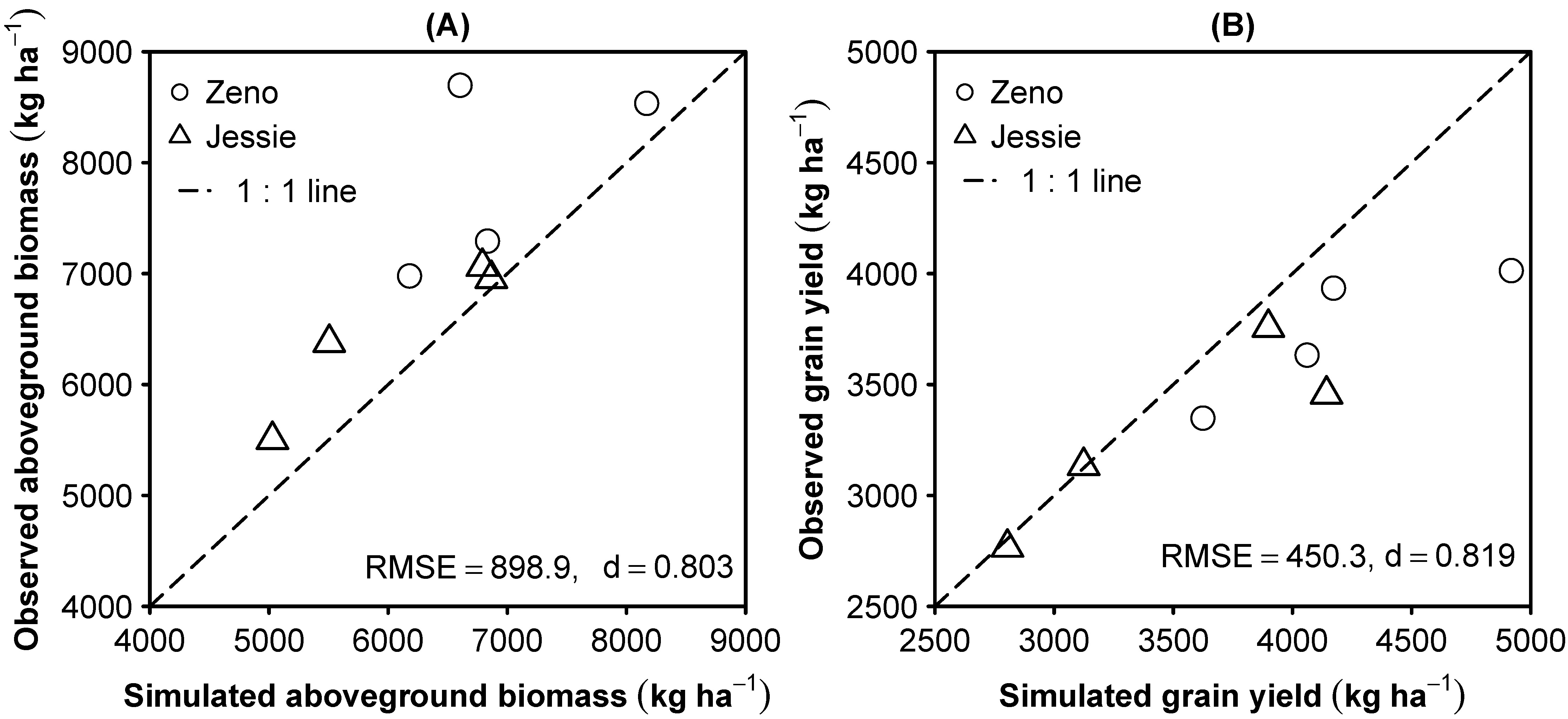
3.2. Model Evaluation

The model evaluation of quinoa phenology across four sowing dates in 2017 showed highly accurate predictions of the first pod date, anthesis date, and harvest maturity date (Figure 11). Averaged across all sowing dates, the simulated first pod date was 54 days after sowing (DAS) for both cultivars and thus very close to the observed mean value of the first pod appearance at 50 (cv. Zeno) and 52 (cv. Jessie) DAS, giving an overall RMSE of 3.0 days. Similarly, the simulated mean anthesis date was 62 DAS for both cultivars compared to the mean values of the observed anthesis at 63 (cv. Zeno) and 62 (cv. Jessie) DAS with an overall RMSE of 1.5 days. The simulated mean harvest maturity date at 114 DAS for cv. Jessie matched the observed mean value for this cultivar. In contrast, the simulated harvest maturity for cv. Zeno was 118 DAS, while the observed mean harvest maturity date was 113 DAS. On average (both cultivars, all sowing dates) the RMSE for the harvest maturity date was 4.4 days with a corresponding d-index of 0.977. In general, there was a higher accuracy in predicting the phenological stages of quinoa during the evaluation year (2017) compared with the adaptation year (2016). This could be attributed to the higher maximum and minimum temperatures observed in 2017 (Table 5), which might have led to better predictions by the CROPGRO model.

To evaluate the model performance in predicting the potential aboveground biomass and grain yield formation, final values of the four sowing dates in 2017, observed at harvest maturity, were plotted against the corresponding simulated values (Figure 12). For both cultivars, the simulations accurately reflected the lower biomass and yield potential of early sowing dates observed in 2017. However, the model tended toward a slight underestimation of the total aboveground biomass, while the grain yield, especially for late sowing dates, was slightly overestimated. Across all sowing dates, the observed mean values of the total aboveground biomass were 7879 (cv. Zeno) and 6474 kg ha⁻¹ (cv. Jessie) compared to the simulated values of 6946 and 6048 kg ha⁻¹ for cv. Zeno and cv. Jessie, respectively. Overall, the RMSE for both cultivars was 898.9 kg ha⁻¹ with a d-index of 0.803. Regarding the grain yield, a mean value of 3734 (cv. Zeno) and 3278 kg ha⁻¹ (cv. Jessie) was observed across all sowing dates. The corresponding simulated values were very close with 4194 and 3492 kg ha⁻¹ for cv. Zeno and cv. Jessie, respectively. The evaluation statistics showed an overall RMSE of 450.3 kg ha⁻¹ with a d-index of 0.819. In conclusion, the good predictions of life cycle, grain yield, and aboveground biomass for different sowing dates during 2017, which showed remarkably different environmental conditions compared with 2016 (Table 5), confirmed the suggested exceptional performance of the new quinoa model.

4. Conclusions

A new CROPGRO model for quinoa was developed to support research, and consequently, the introduction of a potential crop in European cropping systems suitable for dealing with unfavorable environmental conditions. The model offers a good starting point to integrate further knowledge on quinoa physiology while providing the possibility to evaluate the long-term suitability and different management strategies of quinoa under European conditions. The model adaptation based on the modification of numerous species and genetic traits resulted in reasonable simulations of the crop’s phenological (phase durations of different development stages, leaf number, etc.), physiological (N-mobilization), and growth (LAI, SLA, aboveground biomass, yield, etc.) parameters. Since the adaptation and evaluation was performed for two cultivars across different sowing dates, giving various environmental conditions, our results suggest a good robustness of the new quinoa model. However, it was based on one field trial and one location, and should therefore be further improved and evaluated using other cultivars and growth analysis data generated under differing (unfavorable) environmental conditions with special attention to drought. Additionally, reformulation of the model code is needed to simulate small seed sizes and thus to improve the model accuracy regarding reproductive partitioning. Since we assumed no N-limitation during the adaptation and evaluation process, another important model area that needs to be introduced for quinoa includes the response to N fertilization. Therefore, the DSSAT soil C module, or rather the associated routines used for N mineralization, have to be reevaluated, and the source code possibly has to be changed to reach sufficient soil N mineralization. Further improvements and evaluation of this new quinoa model would be facilitated through the inclusion into the next DSSAT version.

References

1. Olesen, J.E.; Trnka, M.; Kersebaum, K.C.; Skjelvåg, A.O.; Seguin, B.; Peltonen-Sainio, P.; Rossi, F.; Kozyra, J.; Micale, F. Impacts and adaptation of European crop production systems to climate change. Eur. J. Agron. 2011, 34, 96–112. [Google Scholar] [CrossRef]
2. Rosenzweig, C.; Iglesias, A.; Yang, X.B.; Epstein, P.R.; Chivian, E. Climate change and extreme weather events; implications for food production, plant diseases, and pests. Glob. Chang. Hum. Health 2001, 2, 90–104. [Google Scholar] [CrossRef]
3. Olesen, J.E.; Bindi, M. Consequences of climate change for European agricultural productivity, land use and policy. Eur. J. Agron. 2002, 16, 239–262. [Google Scholar] [CrossRef]
4. Rezaei, E.E.; Gaiser, T.; Siebert, S.; Ewert, F. Adaptation of crop production to climate change by crop substitution. Mitig. Adapt. Strateg. Glob. Chang. 2015, 20, 1155–1174. [Google Scholar] [CrossRef]
5. Turral, H.; Burke, J.; Faurès, J.M. Climate change, water and food security. In FAO Water Reports No. 36; FAO: Rome, Italy, 2011. [Google Scholar]
6. Smit, B.; Skinner, M.W. Adaptation options in agriculture to climate change: A typology. Mitig. Adapt. Strateg. Glob. Chang. 2002, 7, 85–114. [Google Scholar] [CrossRef]
7. Bazile, D.; Bertero, D.; Nieto, C. State of the Art Report of Quinoa in the World in 2013, In FAO & CIRAD 2015; FAO: Rome, Italy, 2015; ISBN 978-92-5-108558-5. [Google Scholar]
8. Ruiz, K.B.; Biondi, S.; Oses, R.; Acuña-Rodríguez, I.S.; Antognoni, F.; Martinez-Mosqueira, E.A.; Coulibaly, A.; Canahua-Murillo, A.; Pinto, M.; Zurita-Silva, A.; et al. Quinoa biodiversity and sustainability for food security under climate change. A review. Agron. Sustain. Dev. 2014, 34, 349–359. [Google Scholar] [CrossRef]
9. Fuentes, F.F.; Bazile, D.; Bhargava, A.; Martínez, E.A. Implications of farmers’ seed exchanges for on-farm conservation of quinoa, as revealed by its genetic diversity in Chile. J. Agric. Sci. 2012, 150, 702–716. [Google Scholar] [CrossRef]
10. Bazile, D.; Fuentes, F.; Mujica, A. Historical Perspectives and Domestication. In Quinoa: Botany, Production and Uses; Bhargava, A., Srivastava, S., Eds.; CAB International: Wallingford, Oxfordshire, UK, 2013; pp. 16–36. ISBN 978-1-78064-226-0. [Google Scholar]
11. Bazile, D.; Martínez, E.A.; Fuentes, F. Diversity of quinoa in a biogeographical Island: A review of constraints and potential from arid to temperate regions of Chile. Not. Bot. Horti Agrobot. Cluj Napoca 2014, 42, 289–298. [Google Scholar] [CrossRef]
12. Jacobsen, S.E.; Mujica, A.; Jensen, C.R. The resistance of quinoa (Chenopodium quinoa Willd.) to adverse abiotic factors. Food Rev. Int. 2003, 19, 99–109. [Google Scholar] [CrossRef]
13. Martínez, E.A.; Veas, E.; Jorquera, C.; San Martín, R.; Jara, P. Re-introduction of quinoa into Arid Chile: Cultivation of two lowland races under extremely low irrigation. J. Agron. Crop. Sci. 2009, 195, 1–10. [Google Scholar] [CrossRef]
14. Sanchez, H.B.; Lemeur, R.; Damme, P.V.; Jacobsen, S.E. Ecophysiological analysis of drought and salinity stress of quinoa (Chenopodium quinoa Willd.). Food Rev. Int. 2003, 19, 111–119. [Google Scholar] [CrossRef]
15. Cocozza, C.; Pulvento, C.; Lavini, A.; Riccardi, M.; d’Andria, R.; Tognetti, R. Effects of Increasing Salinity Stress and Decreasing Water Availability on Ecophysiological Traits of Quinoa (Chenopodium quinoa Willd.) Grown in a Mediterranean-Type Agroecosystem. J. Agron. Crop. Sci. 2013, 199, 229–240. [Google Scholar] [CrossRef]
16. Bois, J.F.; Winkel, T.; Lhomme, J.P.; Raffaillac, J.P.; Rocheteau, A. Response of some Andean cultivars of quinoa (Chenopodium quinoa Willd.) to temperature: Effects on germination, phenology, growth and freezing. Eur. J. Agron. 2006, 25, 299–308. [Google Scholar] [CrossRef]
17. Präger, A.; Munz, S.; Nkebiwe, P.; Mast, B.; Graeff-Hönninger, S. Yield and quality characteristics of different quinoa (Chenopodium quinoa Willd.) Cultivars grown under field conditions in Southwestern Germany. Agronomy 2018, 8, 197. [Google Scholar] [CrossRef]
18. Prego, I.; Maldonado, S.; Otegui, M. Seed structure and localization of reserves in Chenopodium quinoa. Ann. Bot. 1998, 82, 481–488. [Google Scholar] [CrossRef]
19. McDonell, E. Nutrition Politics in the Quinoa Boom: Connecting Consumer and Producer Nutrition in the Commercialization of Traditional Foods. Int. J. Food. Nutr. Sci. 2016, 3, 1–7. [Google Scholar] [CrossRef]
20. Furche, C.; Salcedo, S.; Krivonos, E.; Rabczuk, P.; Jara, B.; Fernandez, D.; Correa, F. International Quinoa trade. In State of the Art Report of Quinoa in the World in 2013; Bazile, D., Bertero, D., Nieto, C., Eds.; FAO & CIRAD: Rome, Italy, 2015; pp. 316–329. ISBN 978-92-5-108558-5. [Google Scholar]
21. Noulas, C.; Tziouvalekas, M.; Vlachostergios, D.; Baxevanos, D.; Karyotis, T.; Iliadis, C. Adaptation, agronomic potential, and current perspectives of quinoa under mediterranean conditions: Case studies from the lowlands of central Greece. Commun. Soil Sci. Plant Anal. 2017, 48, 2612–2629. [Google Scholar] [CrossRef]
22. Szilagyi, L.; Jørnsgǻrd, B. Preliminary agronomic evaluation of Chenopodium quinoa Willd. under climatic conditions of Romania. Sci. Pap. Ser. A Agron. 2014, 57, 339–343. [Google Scholar]
23. Stikic, R.; Glamoclija, D.; Demin, M.; Vucelic-Radovic, B.; Jovanovic, Z.; Milojkovic-Opsenica, D.; Jacobsen, S.E.; Milovanovic, M. Agronomical and nutritional evaluation of quinoa seeds (Chenopodium quinoa Willd.) as an ingredient in bread formulations. J. Cereal Sci. 2012, 55, 132–138. [Google Scholar] [CrossRef]
24. Pulvento, C.; Riccardi, M.; Lavini, A.; d’Andria, R.; Iafelice, G.; Marconi, E. Field trial evaluation of two chenopodium quinoa genotypes grown under rain-fed conditions in a typical Mediterranean environment in South Italy. J. Agron. Crop. Sci. 2010, 196, 407–411. [Google Scholar] [CrossRef]
25. Bazile, D.; Pulvento, C.; Verniau, A.; Al-Nusari, M.S.; Ba, D.; Breidy, J.; Hassan, L.; Mohammed, M.I.; Mambetov, O.; Sepahvand, N.A.; et al. Worldwide Evaluations of Quinoa: Preliminary Results from Post International Year of Quinoa FAO Projects in Nine Countries. Front. Plant Sci. 2016, 7, 1–18. [Google Scholar] [CrossRef] [PubMed]
26. Singh, S.; Boote, K.J.; Angadi, S.V.; Grover, K.; Begna, S.; Auld, D. Adapting the CROPGRO model to simulate growth and yield of spring safflower in semiarid conditions. Agron. J. 2016, 108, 64–72. [Google Scholar] [CrossRef]
27. Blade, S.F.; Slinkard, A.E. New crop development: The Canadian experience. In Trends in New Crops and New Uses; Janick, J., Whipkey, A., Eds.; ASHS Press: Alexandria, VA, USA, 2002; pp. 62–75. ISBN 0-970756-5-5. [Google Scholar]
28. Fodor, N.; Challinor, A.; Droutsas, I.; Ramirez-Villegas, J.; Zabel, F.; Koehler, A.K.; Foyer, C.H. Integrating plant science and crop modeling: Assessment of the impact of climate change on soybean and maize production. Plant Cell Physiol. 2017, 58, 1833–1847. [Google Scholar] [CrossRef] [PubMed]
29. Ma, L.; Ahuja, L.R.; Islam, A.; Trout, T.J.; Saseendran, S.A.; Malone, R.W. Modeling yield and biomass responses of maize cultivars to climate change under full and deficit irrigation. Agric. Water Manag. 2017, 180, 88–98. [Google Scholar] [CrossRef]
30. Attia, A.; Rajan, N.; Xue, Q.; Nair, S.; Ibrahim, A.; Hays, D. Application of DSSAT-CERES-Wheat model to simulate winter wheat response to irrigation management in the Texas High Plains. Agric. Water Manag. 2016, 165, 50–60. [Google Scholar] [CrossRef]
31. Ewert, F.; Rötter, R.P.; Bindi, M.; Webber, H.; Trnka, M.; Kersebaum, K.C.; Olesen, J.E.; van Ittersum, M.K.; Janssen, S.; Rivington, M.; et al. Crop modelling for integrated assessment of risk to food production from climate change. Environ. Model. Softw. 2015, 72, 287–303. [Google Scholar] [CrossRef]
32. Ngwira, A.R.; Aune, J.B.; Thierfelder, C. DSSAT modelling of conservation agriculture maize response to climate change in Malawi. Soil Till. Res. 2014, 143, 85–94. [Google Scholar] [CrossRef]
33. Zamora, D.S.; Jose, S.; Jones, J.W.; Cropper, W.P. Modeling cotton production response to shading in a pecan alleycropping system using CROPGRO. Agrofor. Syst. 2009, 76, 423–435. [Google Scholar] [CrossRef]
34. Boote, K.J.; Jones, J.W.; Pickering, N.B. Potential uses and limitations of crop models. Agron. J. 1996, 88, 704–716. [Google Scholar] [CrossRef]
35. Geerts, S.; Raes, D.; Garcia, M.; Miranda, R.; Cusicanqui, J.A.; Taboada, C.; Mendoza, J.; Huanca, R.; Mamani, A.; Condori, O.; et al. Simulating yield response of quinoa to water availability with AquaCrop. Agron. J. 2009, 101, 499–508. [Google Scholar] [CrossRef]
36. Geerts, S.; Raes, D.; Garcia, M.; Taboada, C.; Miranda, R.; Cusicanqui, J.; Mhizha, T.; Vacher, J. Modeling the potential for closing quinoa yield gaps under varying water availability in the Bolivian Altiplano. Agric. Water Manag. 2009, 96, 1652–1658. [Google Scholar] [CrossRef]
37. Hirich, A.; Choukr-Allah, R.; Ragab, R.; Jacobsen, S.E.; El Youssfi, L.; El Omari, H. The SALTMED model calibration and validation using field data from Morocco. J. Mater. Environ. Sci. 2012, 3, 342–359. [Google Scholar]
38. Pulvento, C.; Riccardi, M.; Lavini, A.; D’andria, R.; Ragab, R. SALTMED model to simulate yield and dry matter for quinoa crop and soil moisture content under different irrigation strategies in south Italy. Irrig. Drain. 2013, 62, 229–238. [Google Scholar] [CrossRef] [Green Version]
39. Fghire, R.; Wahbi, S.; Anaya, F.; Issa Ali, O.; Benlhabib, O.; Ragab, R. Response of quinoa to different water management strategies: Field experiments and SALTMED model application results. Irrig. Drain. 2015, 64, 29–40. [Google Scholar] [CrossRef]
40. Kaya, Ç.I.; Yazar, A.; Sezen, S.M. SALTMED model performance on simulation of soil moisture and crop yield for quinoa irrigated using different irrigation systems, irrigation strategies and water qualities in Turkey. Agric. Agricu. Sci. Procedia 2015, 4, 108–118. [Google Scholar] [CrossRef]
41. Kaya, Ç.I.; Yazar, A. SALTMED model performance for quinoa irrigated with fresh and saline water in a Mediterranean environment. Irrig. Drain. 2016, 65, 29–37. [Google Scholar] [CrossRef]
42. Steduto, P.; Raes, D.; Hsiao, T.C.; Fereres, E.; Heng, L.K.; Howell, T.A.; Evett, S.R.; Rojas-Lara, B.A.; Farahani, H.J.; Izzi, G.; et al. Concepts and applications of AquaCrop: The FAO crop water productivity model. In Crop Modeling and Decision Support; Cao, W., White, J.W., Wang, E., Eds.; Springer: Berlin/Heidelberg, Germany, 2009; pp. 175–191. ISBN 978-3-642-01132-0. [Google Scholar]
43. Ragab, R. Integrated management tool for water, crop, soil and N-fertilizers: The SALTMED model. Irrig. Drain. 2015, 64, 1–12. [Google Scholar] [CrossRef] [Green Version]
44. Ragab, R. A holistic generic integrated approach for irrigation, crop and field management: The SALTMED model. Environ. Model. Softw. 2002, 17, 345–361. [Google Scholar] [CrossRef]
45. Hassanli, M.; Ebrahimian, H.; Mohammadi, E.; Rahimi, A.; Shokouhi, A. Simulating maize yields when irrigating with saline water, using the AquaCrop, SALTMED, and SWAP models. Agric. Water Manag. 2016, 176, 91–99. [Google Scholar] [CrossRef]
46. Jones, J.W.; Hoogenboom, G.; Porter, C.H.; Boote, K.J.; Batchelor, W.D.; Hunt, L.A.; Wilkens, P.W.; Singh, U.; Gijsman, A.J.; Ritchie, J.T. The DSSAT cropping system model. Eur. J. Agron. 2003, 18, 235–265. [Google Scholar] [CrossRef]
47. Boote, K.J.; Jones, J.W.; Hoogenboom, G. Simulation of crop growth: CROPGRO model. In Agricultural Systems Modeling and Simulation; Peart, R.M., Curry, R.B., Eds.; Marcel Dekker Inc.: New York, NY, USA, 1998; pp. 651–692. ISBN 0824700414. [Google Scholar]
48. Boote, K.J.; Jones, J.W.; Hoogenboom, G.; Pickering, N.B. The CROPGRO model for grain legumes. In Understanding Options for Agricultural Production; Tsuji, G.Y., Hoogenboom, G., Thornton, P.K., Eds.; Springer Science+Business Media: Berlin/Heidelberg, Germany, 1998; pp. 99–128. ISBN 978-94-017-3624-4. [Google Scholar]
49. Hoogenboom, G.; Porter, C.H.; Shelia, V.; Boote, K.J.; Singh, U.; White, J.W.; Hunt, L.A.; Ogoshi, R.; Lizaso, J.I.; Koo, J.; et al. Decision Support System for Agrotechnology Transfer (DSSAT) Version 4.7 (www.DSSAT.net); DSSAT Foundation: Gainesville, FL, USA, 2017. [Google Scholar]
50. Boote, K.J.; Mínguez, M.I.; Sau, F. Adapting the CROPGRO legume model to simulate growth of faba bean. Agron. J. 2002, 94, 743–756. [Google Scholar] [CrossRef]
51. Alderman, P.D.; Boote, K.J.; Jones, J.W.; Bhatia, V.S. Adapting the CSM-CROPGRO model for pigeonpea using sequential parameter estimation. Field Crop. Res. 2015, 181, 1–15. [Google Scholar] [CrossRef]
52. Deligios, P.A.; Farci, R.; Sulas, L.; Hoogenboom, G.; Ledda, L. Predicting growth and yield of winter rapeseed in a Mediterranean environment: Model adaptation at a field scale. Field Crop. Res. 2013, 144, 100–112. [Google Scholar] [CrossRef]
53. Pathak, T.B.; Jones, J.W.; Fraisse, C.W.; Wright, D.; Hoogenboom, G. Uncertainty analysis and parameter estimation for the CSM-CROPGRO-Cotton model. Agron. J. 2012, 104, 1363–1373. [Google Scholar] [CrossRef] [Green Version]
54. Pedreira, B.C.; Pedreira, C.G.; Boote, K.J.; Lara, M.A.; Alderman, P.D. Adapting the CROPGRO perennial forage model to predict growth of Brachiaria brizantha. Field Crop. Res. 2011, 120, 370–379. [Google Scholar] [CrossRef]
55. Hartkamp, A.D.; Hoogenboom, G.; White, J.W. Adaptation of the CROPGRO growth model to velvet bean (Mucuna pruriens): I. Model development. Field Crop. Res. 2002, 78, 9–25. [Google Scholar] [CrossRef]
56. Jacobsen, S.E. The scope for adaptation of quinoa in Northern Latitudes of Europe. J. Agron. Crop. Sci. 2017, 203, 603–613. [Google Scholar] [CrossRef]
57. IUSS Working Group WRB. World Reference Base for Soil Resources 2006, First Update 2007. In World Soil Resources Reports No. 103; FAO: Rome, Italy, 2007. [Google Scholar]
58. Jacobsen, S.E.; Stølen, O. Quinoa—Morphology, phenology and prospects for its production as a new crop in Europe. Eur. J. Agron. 1993, 2, 19–29. [Google Scholar] [CrossRef]
59. Sosa-Zuniga, V.; Brito, V.; Fuentes, F.; Steinfort, U. Phenological growth stages of quinoa (Chenopodium quinoa) based on the BBCH scale. Ann. Appl. Biol. 2017, 171, 117–124. [Google Scholar] [CrossRef]
60. AOAC. Official Methods of Analysis, 15th ed.; Association of Official Analytical Chemists, Inc.: Arlington, TX, USA, 1990; p. 70. ISBN 0-935584-42-0. [Google Scholar]
61. Fensterseifer, C.A.; Streck, N.A.; Baigorria, G.A.; Timilsina, A.P.; Zanon, A.J.; Cera, J.C.; Rocha, T.S. On the number of experiments required to calibrate a cultivar in a crop model: The case of CROPGRO-soybean. Field Crop. Res. 2017, 204, 146–152. [Google Scholar] [CrossRef]
62. Willmott, C.J. Some comments on the evaluation of model performance. Bull. Am. Meteorol. Soc. 1982, 63, 1309–1313. [Google Scholar] [CrossRef] [Green Version]
63. Jacobsen, S.E.; Bach, A.P. The influence of temperature on seed germination rate in quinoa (Chenopodium quinoa Willd.). Seed Sci. Technol. 1998, 26, 515–523. [Google Scholar]
64. Bertero, H.D.; King, R.W.; Hall, A.J. Photoperiod and temperature effects on the rate of leaf appearance in quinoa (Chenopodium quinoa). Funct. Plant Biol. 2000, 27, 349–356. [Google Scholar] [CrossRef]
65. Bertero, H.D.; King, R.W.; Hall, A.J. Modelling photoperiod and temperature responses of flowering in quinoa (Chenopodium quinoa Willd.). Field Crop. Res. 1999, 63, 19–34. [Google Scholar] [CrossRef]
66. Bertero, H.D. Environmental Control of Development. In State of the Art Report of Quinoa in the World in 2013; Bazile, D., Bertero, D., Nieto, C., Eds.; FAO & CIRAD: Rome, Italy, 2015; pp. 120–130. ISBN 978-92-5-108558-5. [Google Scholar]
67. Bertero, H.D.; King, R.W.; Hall, A.J. Photoperiod-sensitive development phases in quinoa (Chenopodium quinoa Willd.). Field Crop. Res. 1999, 60, 231–243. [Google Scholar] [CrossRef]
68. Walters, H.; Carpenter-Boggs, L.; Desta, K.; Yan, L.; Matanguihan, J.; Murphy, K. Effect of irrigation, intercrop, and cultivar on agronomic and nutritional characteristics of quinoa. Agroecol. Sustain. Food Syst. 2016, 40, 783–803. [Google Scholar] [CrossRef]
69. Hafid, R.E.; Imaalem, H.A.; Driedger, D.; Bandara, M.; Stevenson, J. Quinoa…The next Cinderella crop for Alberta? Alberta Agric. Food Rural Dev. 2005, 1–28. Available online: https://www1.agric.gov.ab.ca/$department/deptdocs.nsf/all/afu9961/$FILE/quinoa_final_report_june_05.pdf (accessed on 1 December 2019).
70. Hinojosa, L.; Matanguihan, J.B.; Murphy, K.M. Effect of high temperature on pollen morphology, plant growth and seed yield in quinoa (Chenopodium quinoa Willd). J. Agron. Crop. Sci. 2019, 205, 33–45. [Google Scholar] [CrossRef] [Green Version]
71. Bunce, J.A. Variation in yield responses to elevated CO2 and a brief high temperature treatment in quinoa. Plants 2017, 6, 26. [Google Scholar] [CrossRef] [Green Version]
72. Yang, A.; Akhtar, S.S.; Amjad, M.; Iqbal, S.; Jacobsen, S.E. Growth and physiological responses of quinoa to drought and temperature stress. J. Agron. Crop. Sci. 2016, 202, 445–453. [Google Scholar] [CrossRef]
73. Bunce, J.A. Thermal acclimation of the temperature dependence of the VCmax of Rubisco in quinoa. Photosynthetica 2018, 56, 1171–1176. [Google Scholar] [CrossRef]
74. Pearcy, R.W.; Tumosa, N.; Williams, K. Relationships between growth, photosynthesis and competitive interactions for a C 3 and C 4 plant. Oecologia 1981, 48, 371–376. [Google Scholar] [CrossRef] [PubMed]
75. Penning de Vries, F.W.T.; van Laar, H.H. Simulation of growth processes and the model BACROS. In Simulation of Plant Growth and Crop Production; Penning de Vries, F.W.T., van Laar, H.H., Eds.; PUDOC: Wageningen, The Netherlands, 1982; pp. 114–136. ISBN 9789022008096. [Google Scholar]
76. Ahamed, N.T.; Singhal, R.S.; Kulkarni, P.R.; Pal, M. A lesser-known grain, Chenopodium quinoa: Review of the chemical composition of its edible parts. Food Nutr. Bull. 1998, 19, 61–70. [Google Scholar] [CrossRef]
77. Kozioł, M.J. Chemical composition and nutritional evaluation of quinoa (Chenopodium quinoa Willd.). J. Food Compos. Anal. 1992, 5, 35–68. [Google Scholar] [CrossRef]
78. Bhargava, A.; Shukla, S.; Srivastava, J.; Singh, N.; Ohri, D. Genetic diversity for mineral accumulation in the foliage of Chenopodium spp. Sci. Hortic. 2008, 118, 338–346. [Google Scholar] [CrossRef]
79. Bhargava, A.; Shukla, S.; Ohri, D. Mineral composition in foliage of some cultivated and wild species of Chenopodium. Span. J. Agric. Res. 2010, 8, 371–376. [Google Scholar] [CrossRef] [Green Version]
80. Schlick, G. Nutritional Characteristics and Biomass Production of Chenopodium Quinoa Grown in Controlled Environments. Master’s Thesis, San Jose State University, San Jose, CA, USA, 2000. [Google Scholar]
81. Tang, Y.; Li, X.; Chen, P.X.; Zhang, B.; Hernandez, M.; Zhang, H.; Marcone, M.F.; Liu, R.; Tsao, R. Lipids, tocopherols, and carotenoids in leaves of amaranth and quinoa cultivars and a new approach to overall evaluation of nutritional quality traits. J. Agric. Food Chem. 2014, 62, 12610–12619. [Google Scholar] [CrossRef]
82. Carrasco, C.; Cuno, D.; Carlqvist, K.; Galbe, M.; Lidén, G. SO2-catalysed steam pretreatment of quinoa stalks. J. Chem. Technol. Biotechnol. 2015, 90, 64–71. [Google Scholar] [CrossRef]
83. Boote, K.J.; Pickering, N.B. Modeling photosynthesis of row crop canopies. HortScience 1994, 29, 1423–1434. [Google Scholar] [CrossRef] [Green Version]
84. Bascuñán-Godoy, L.; Sanhueza, C.; Pinto, K.; Cifuentes, L.; Reguera, M.; Briones, V.; Zurita-Silva, A.; Álvarez, R.; Morales, A.; Silva, H. Nitrogen physiology of contrasting genotypes of Chenopodium quinoa Willd.(Amaranthaceae). Sci. Rep. 2018, 8, 1–12. [Google Scholar] [CrossRef]
85. Jacobsen, S.E.; Monteros, C.; Corcuera, L.J.; Bravo, L.A.; Christiansen, J.L.; Mujica, A. Frost resistance mechanisms in quinoa (Chenopodium quinoa Willd.). Eur. J. Agron. 2007, 26, 471–475. [Google Scholar] [CrossRef]
Figure 1. A comparison between the simulated and observed days after sowing (DAS) to first pod (A), to first anthesis (B), and to harvest maturity (C) for the adapted quinoa cultivars Zeno and Jessie sown on four different dates in 2016, where RMSE: root mean square error and d: Willmott agreement index.
Agronomy 09 00832 g001
Figure 2. A comparison between the simulated (Sim) and observed (Obs) main stem leaf number (1) and plant height (2) for the adapted quinoa cultivars Zeno (A) and Jessie (B) sown on four different dates (SD) in 2016 as a function of days after sowing, where RMSE: root mean square error and d: Willmott agreement index.
Agronomy 09 00832 g002
Figure 3. A comparison between the simulated (Sim) and observed (Obs) specific leaf area for the adapted quinoa cultivars Zeno (A) and Jessie (B) sown on four different dates (SD) in 2016 as a function of days after sowing, where RMSE: root mean square error and d: Willmott agreement index.
Agronomy 09 00832 g003
Figure 4. A comparison between the simulated (Sim) and observed (Obs) leaf area index for the adapted quinoa cultivars Zeno (A) and Jessie (B) sown on four different dates (SD) in 2016 as a function of days after sowing, where RMSE: root mean square error and d: Willmott agreement index.
Agronomy 09 00832 g004
Figure 5. A comparison between the simulated (Sim) and observed (Obs) leaf weight (1) and stem weight (2) for the adapted quinoa cultivars Zeno (A) and Jessie (B) sown on four different dates (SD) in 2016 as a function of days after sowing, where RMSE: root mean square error and d: Willmott agreement index.
Agronomy 09 00832 g005
Figure 6. A comparison between the simulated (Sim) and observed (Obs) leaf nitrogen concentration for the adapted quinoa cultivars Zeno (A) and Jessie (B) sown on four different dates (SD) in 2016 as a function of days after sowing, where RMSE: root mean square error and d: Willmott agreement index.
Agronomy 09 00832 g006
Figure 7. A comparison between the simulated (Sim) and observed (Obs) grain to pod ratio for the adapted quinoa cultivars Zeno (A) and Jessie (B) sown on four different dates (SD) in 2016 as a function of days after sowing, where RMSE: root mean square error and d: Willmott agreement index.
Agronomy 09 00832 g007
Figure 8. A comparison between the simulated (Sim) and observed (Obs) pod harvest index (1) and grain harvest index (2) for the adapted quinoa cultivars Zeno (A) and Jessie (B) sown on four different dates (SD) in 2016 as a function of days after sowing, where RMSE: root mean square error and d: Willmott agreement index.
Agronomy 09 00832 g008
Figure 9. A comparison between the simulated (Sim) and observed (Obs) pod weight (1) and grain weight (2) for the adapted quinoa cultivars Zeno (A) and Jessie (B) sown on four different dates (SD) in 2016 as a function of days after sowing, where RMSE: root mean square error and d: Willmott agreement index.
Agronomy 09 00832 g009
Figure 10. A comparison between the simulated (Sim) and observed (Obs) aboveground biomass for the adapted quinoa cultivars Zeno (A) and Jessie (B) sown on four different dates (SD) in 2016 as a function of days after sowing, where RMSE: root mean square error and d: Willmott agreement index.
Agronomy 09 00832 g010
Figure 11. A comparison between the simulated and observed days after sowing (DAS) to first pod (A), to first anthesis (B), and to harvest maturity (C) for the evaluated quinoa cultivars Zeno and Jessie sown on four different dates in 2017, where RMSE: root mean square error and d: Willmott agreement index.
Agronomy 09 00832 g011
Figure 12. A comparison between the simulated and observed aboveground biomass (A) and grain yield (B) at harvest maturity for the evaluated quinoa cultivars Zeno and Jessie sown on four different dates in 2017, where RMSE: root mean square error and d: Willmott agreement index.
Agronomy 09 00832 g012