Price Forecasting and Span Commercialization Opportunities for Mexican Agricultural Products

Abstract

Decision-making based on data analysis leads to knowing market trends and anticipating risks and opportunities. These allow farmers to improve their production plan as well as their chances to get an economic success. The aim of this work was to develop a methodology for price forecasting of fruits and vegetables using Queretaro state, MX as a case study. The daily prices of several fruits and vegetables were extracted, from January 2009 to February 2019, from the National System of Market Information. Then, these prices were used to compute the weekly average price of each product and their span commercialization in Q4 and over the median of historical data. Moreover, product characterization was performed to propose a methodology for future price forecasting of multiple agricultural products within the same mathematical model and it resulted in the identification of 18 products that fit the Seasonal Auto-Regressive Integrated Moving Average (SARIMA) model. Finally, future price estimation and validation was performed to explain the product price fluctuations between weeks and it was found that the relative error for most of products modeled was less than 10%, e.g., Hass avocado (7.01%) and Saladette tomato (8.09%). The results suggest the feasibility for the implementation of systems to provide information for better decisions by Mexican farmers.

1. Introduction

Agriculture production plays a key role in food security and economy of a country [1]. In 2017, the agriculture sector contributed 3.55% to the Gross Domestic Product (GDP) of the world [2]. Meanwhile, in Mexico, 21.6 million hectares were allocated for agriculture production and they contributed to 3.35% to the GDP [2,3]. The Mexican agro-industrial trade balance has increased throughout the years. In 2018, it resulted in 34,255 million USD from exports and 28,416 million USD from imports [4].

Price short-term forecasting models and methods for fruits and vegetables have been studied since the 21st century [5]. These models and methods can be divided into price forecasting methods based on Artificial Neural Networks (ANNs) and models based on the Box–Jenkins methodology. However, the parameters of each model change between zones. For example, the monthly price of tomato was modeled using an ARIMA(23,0,1) in Mexico [6] and a SARIMA(0,1,2,1,1,1,1) in China [5]. Moreover, the usefulness of these approaches depends of the local market context. For example, in China, the high volatility of the prices lead to ANN models or hybrid models to get a better fit than the Box–Jenkins methodology [7,8].

Moreover, one of the price forecasting goals is to provide information to help Mexican farmers. In this way, there are several case studies designed to provide technical support for business decisions in the agriculture sector by price forecasting. However, most case studies aim at price prediction for only one or two products, e.g. the price of onion [9], the price of cabbage [10], the price of pepper [10,11], the price of cucumber [10], the price of green bean [10], and the price of tomato [5,6,10,11,12,13,14]. In this way, even if the error in the price prediction were low, farmers would not know alternative products to sow when the product prices are anticipated to decrease. Therefore, an extensive analysis and price forecasting for more than one or two products is mandatory. On the other hand, ANNs models do not enable researchers to understand the market dynamics since ANNs are black-box models [12]. For example, ANNs do not allow the existence of seasonal trends of products (usually an annual season).

In this work, Queretaro state was selected as a case study. Its data were taken from the National System of Information and Integration of markets in Mexico (known as SNIIM). These data were filtered by different methods to determine which of these products had enough data to employ the Box–Jenkins methodology. Then, the prices of the products that met this criteria were analyzed to find their weekly commercialization span opportunities and to develop a model based on Box–Jenkins methodology, which can be applied to understand the market dynamics of the prices of these products. Finally, these products were classified according to the degree of complexity of their model.

2. Methodology

In this work, we used a data workflow based on proposal of McKinney [15], which consists in two main stages: (1) the pre-processing stage, which involves data extraction, filtering, and processing; and (2) the computation stage, which involves the model estimation. The employed data workflow is described in Figure 1.

2.1. Data Extraction

The products’ daily prices were extracted using Python’s lxml library from the SNIIM’s website (http://www.economia-sniim.gob.mx/). This website provides daily information about several fruits and vegetables from many wholesale food markets in Mexico: price, packaging, origin, and quality.

• Price. According to SNIIM, the products’ daily prices are only collected on work days (which in Mexico represents approximately 70% of the year).
• Packaging. It refers to the presentation of the product e.g., bunches or boxes.
• Origin. It refers to whether product is local or imported.
• Quality. There are two types: first quality and exportation quality.

The data were only extracted for the time period between 01/Jan/2009 and 28/Feb/2019 for Queretaro’s wholesale food markets. The data from 01/Jan/2009 to 31/Dec/2018 were used as the train dataset and the remaining data were used as test dataset.

2.2. Data Filtering

Missing data. Eighty-five different products were classified according to the amount of missing data, i.e., the number of days when the data of the product were not available. They were grouped as follows:

• Persistent. A product is called persistent when the missing data in the last four years do not exceed 30%.
• Seasonal. A product is called seasonal when the missing data in the last four years exceed 30%, but present periodical records during the same months year after year.
• Random. A product is called random when the missing data in the last four years exceed 30%, but do not present periodical records during the same months year after year.
• New A product is called new when it has been commercialized for less than four years and the missing data do not exceed 30 % since its commercialization began.
• Dead A product is called dead when there are no data available in the last two years.
• Ghostly. A product is called ghostly when there are fewer than 10 records.

Overall, 48 persistent products, 6 seasonal products, 4 random products, 4 new products, 16 dead products, and 7 ghostly products were found. The detailed list of the products is shown in

Table A1. Groups by filtering missing data.

Label	Products
Persistent	Alpha potato	Ancho pepper	Beet	Bell pepper
	Big-sized cauliflower	Big-sized corn	Big-sized nopal	Big-sized Valencia orange
	Broccoli	Cantaloupe	Celery	Cilantro
	Cucumber	D’ Anjou #100 pear	Dominican banana	Dry puya pepper
	Epazote	Golden delicious apple	Green bean	Green pepper
	Green tomato	Guajillo pepper	Guava	Hass avocado
	Italian zucchini	Jalapeno pepper	Jicama	Kiwi
	Lemon	Lime #5	Male banana	Maradol papaya
	Medium-sized cabbage	Medium-sized carrot	Medium-sized pineapple	No-prickly chayote
	Pasilla pepper	Peanut	Poblano pepper	Radish
	Red delicious apple	Red grapefruit	Romaine big-sized lettuce	Saladette tomato
	Spinach	Strawberry	Stripped watermelon	Tabasco banana.
Seasonal	Ataulfo mango	Castilla pumpkin	Mandarin orange	Manila mango
	Sugarcane	White prickly pear fruit.	Random Balloon grape	Purple garlic
	Superior grape	Thompson grape.
New	Big ball onion	Green bean	Sweet potato	Yellow peach.
Dead	Ball onion	Cantaloupe #12	Cantaloupe #27	Chayote
	Chilaca	Corn	Haden mango	Lime #3
	Medium-sized cauliflower	Medium-sized red grapefruit	Medium-sized Valence orange	Nopal
	Powder carrot	Sangria watermelon	White garlic	Wood carrot.
Ghostly	Big-sized cabbage	Chard	Cherry	Chiapas banana
	Monica orange mandarin	Tamarind	Tejocote.

. Only the persistent products were analyzed.

General classes. One or more products can be classified in “families”, which are “general classes” or “superclasses” that contain related types of products, e.g., white garlic and purple garlic are both types of garlic, therefore both are members of the garlic family and their particular classes are purple and white. However, in some classes, commercialization time intervals are disjoint and one class was substituted by the other one, e.g., lime #3 was substituted by lime #5. Thus, the products were classified into three different families:

• Pure Families that contain only one member.
• Mixed. Families that contain at least two members that do not overlap through time (product replacement).
• Multivalent. Families that contain at least two members that overlap through time.

Overall, 34 products that belonged to a pure family, 21 that belonged to a mixed family, and 30 that belonged to a multivalent family were found. The detailed list of the products is shown in

Table A2. Families by filtering general classes.

Label	Products
Pure Unique	Alpha potato	Beet	Broccoli	Celery
	Cilantro	Cucumber	D’ Anjou #100 pear	Epazote
	Green bean	Green tomato	Guava	Hass avocado
	Italian zucchini	Jicama	Kiwi	Lemon
	Maradol papaya	Medium-sized pineapple	Peanut	Radish
	Romaine big-sized lettuce	Saladette tomato	Spinach	Strawberry
	Castilla pumpkin	Sugarcane	White prickly pear fruit	Green bean
	Sweet potato	Yellow peach	Chard	Cherry
	Tamarind	Tejocote.
Mixed	Ball onion	Big ball onion	Big-sized cauliflower	Big-sized corn
	Big-sized nopal	Big-sized Valencia orange	Cantaloupe	Cantaloupe #12
	Cantaloupe #27	Chayote	Corn	Lime #3
	Lime #5	Medium-sized cauliflower	Medium-sized Valence orange	Nopal
	No-prickly chayote	Purple garlic	Sangria watermelon	Stripped watermelon
	White garlic
Multivalent	Ancho pepper	Ataulfo mango	Balloon grape	Bell pepper
	Big-sized cabbage	Chiapas banana	Chilaca	Dominican banana
	Dry puya pepper	Golden delicious apple	Green pepper	Guajillo pepper
	Haden mango	Jalapeno pepper	Mandarin orange	Male banana
	Manila mango	Medium-sized cabbage	Medium-sized carrot	Medium-sized red grapefruit
	Monica orange mandarin	Pasilla pepper	Poblano pepper	Powder carrot
	Red delicious apple	Red grapefruit	Superior grape	Tabasco banana
	Thompson grape	Wood carrot

. The products that belonged to a pure family, products that belonged to a mixed family, and the substitute products were persistent, and all products that belonged to a multivalent family classified as persistent were analyzed.

Size presentation ambiguity. The presentation of a product in the wholesale food markets may change over time and there may be more than one presentation for the same product. Although most presentations come with an explicit weight description, some presentations are ambiguous, e.g., cilantro was sold as 3 kg bunch, 5 kg bunch, and just a bunch (no weight specified). Since this ambiguity may lead to inconsistent product price analysis, such products were not analyzed. T Five products with ambiguity in their presentation were found.

2.3. Data Processing

Some daily prices remain constant for several days. Thus, the analysis of larger time intervals is equally accurate but more efficient since it leads to less complex models. In this sense, the average price for larger time intervals were computed. However, the use of larger time intervals produces a higher error rate due to the variance increase. In this way, the variance for weekly and monthly time intervals (shown in Figure 2) was computed. It was found that the variance within months is higher than within weeks. Thus, weekly time intervals were selected to be analyzed.

2.4. Span Commercialization Opportunities

Frequency analysis of the prices of each product was performed to determine the weeks within a year with the highest prices. These weeks represent the best chances for farmers to sell their products to increase their profit.

Thus, the weekly prices within a year were sorted from the smallest to the largest. The weekly prices were classified into two categories: good and high. A weekly price was considered “good” when the price is higher than the median of the weekly prices, and was considered “high” when the price is higher than Q3.

According to previous consideration, a week was classified as “a week with a good commercialization opportunity” for a product when its price during that week was “good” for at least nine years, and “a week with a great commercialization opportunity” when its price during that week was “high” for at least seven years. Commercialization opportunities appeared as isolated weeks or as a sequence of several weeks.

There were 35 products with at least three weeks with a good commercialization opportunity, and 22 products with at least three weeks with a high commercialization opportunity (Figure 3).

2.5. Candidate Selection

From the 85 products extracted, only products that were persistent through the years (as explained in Section 2.2), and that belonged to the pure and mixed families (as explained in the general classes section), and that exhibited no ambiguity in their presentation (as explained in size presentation ambiguity), and that presented at least three weeks with a great commercialization opportunity, were analyzed using Box–Jenkins methodology.

2.6. Mathematical Modeling for Price Understanding

Inflation is a reduction in the value of money over a period of time [16]. That is, if the value of a product is constant V, then its price must increase through time. Thus, the price of a product at time t, $P\left(t\right)$ can be modeled as follows:

$$P\left(t\right)=(1+I)P(t-1)$$

(1)

where I is the inflation rate. However, inflation follows the supply and demand for money, but the supply and demand for the product is neglected. Hence, Equation (1) can be modified as follows:

$$P\left(t\right)=(1+I)P(t-1)+C\left(t\right)$$

(2)

where $C\left(t\right)$ is a correction factor that follows the supply and demand for the product. Therefore, the first difference of Equation (2) can be expressed as:

$$\nabla P\left(t\right)=\frac{1}{1+I}\nabla C\left(t\right)$$

(3)

In this way, when the inflation rate I is near 0, the price variations of a product are only consequences of its supply and demand changes. Naturally, the inflation rate is not constant. Nevertheless, in Mexico, the inflation rate has remained almost constant since 2000 [17]. Therefore, Equations (2) and (3) are feasible models.

To understand the price changes of a product, using the Box–Jenkins methodology, auto-correlation (ACF) and partial auto-correlation (PACF) functions must be computed. ACF and PACF according to Shumway and Stoffer can be estimated [18], respectively, as follows:

$$\begin{array}{cc}\hfill \widehat{\rho }\left(h\right)& =\frac{1}{n}\frac{{\sum }_{t=1}^{n-h}\left(x_{t+h}-\overline{x}\right)\left(x_t-\overline{x}\right)}{{\sum }_{t=1}^n\left(x_t-\overline{x}\right)\left(x_t-\overline{x}\right)}\hfill \end{array}$$

(4)

$$\begin{array}{cc}\hfill {\widehat{\varphi }}_{hh}& =\rho \left(x_{t+h}-{\widehat{x}}_{t+h},x_h-{\widehat{x}}_t\right)\hfill \end{array}$$

(5)

where $x_t$ is the observation at time t.

3. Results

Employing Box–Jenkins methodology, the products were classified into three categories: white noise, IMA, and SARIMA. It was not possible to forecast the weekly prices of the products classified as white noise, since the best prediction for their price changes is zero. The products classified as IMA or SARIMA were modeled for future price forecasting and their relative error of the prediction is reported for each case in

Table 1. Relative error for all the selected products.

Product	Model Type	Relative Error
Big Cauliflower	IMA	9.47%
Big Nopal	IMA	34.41%
Big Valencia Orange	SARIMA	3.89%
Epazote	IMA	6.51%
Green Pepper	IMA	36.61%
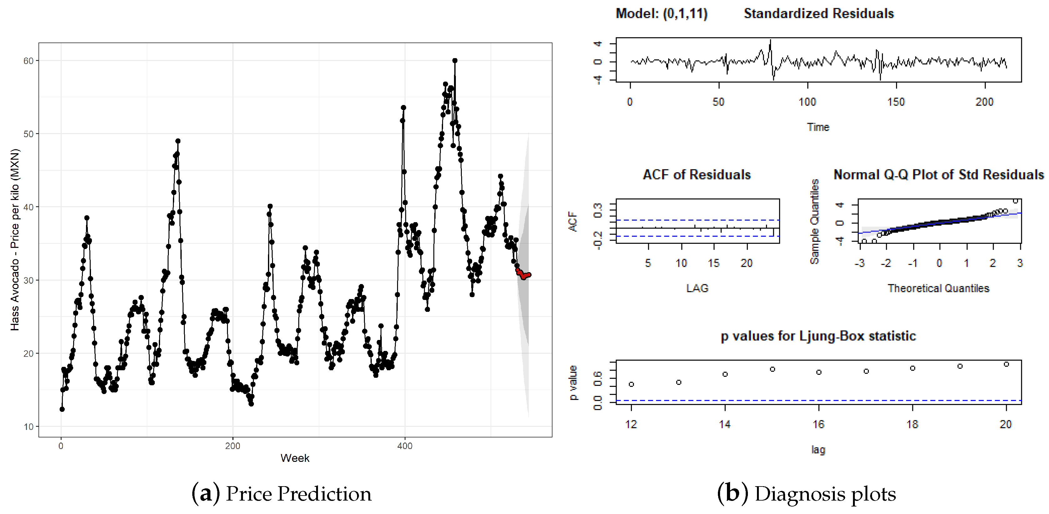
Hass Avocado	IMA	7.01%
Italian Zucchini	IMA	15.91%
Jicama	SARIMA	9.33 %
Kiwi	SARIMA	8.24 %
Lemon	SARIMA	10.07%
Lime #5	SARIMA	6.11%
Male Banana	IMA	4.51%
Medium-sized Pineapple	IMA	4.32%
Non-prickly chayote	IMA	41.39%
Peanut	IMA	3.89%
Red Grapefruit	IMA	3.15%
Saladette Tomato	IMA	8.09%
Tabasco Banana	IMA	23.15%

. In the following paragraphs, the results for each category are presented.

White Noise. Products are classified as white noise when their price changes are statistically similar to a random sample from normal random variable having mean zero. The products that belonged to this category are: D’Anjou pear, Dominican banana, golden apple, red apple, strawberry, and stripped watermelon (most of these products are imported products). To illustrate this category, the stripped watermelon was chosen. Its ACF and PACF (Figure 4) are provided as evidence of its similarity to white noise.

IMA Models. IMA models are a special case of ARIMA where the autoregressive (AR) component is zero. This model is useful to model several economic time series [18]. The following products were modeled successfully: big cauliflower, big nopal, epazote, green pepper, Hass avocado, Italian zucchini, male banana, medium-sized pineapple, no-prickly chayote, peanut, red grapefruit, saladette tomato, and Tabasco banana. To illustrate this model, Hass avocado was chosen. Hass avocado followed an IMA(0,1,11):

$$\nabla P\left(t\right)=w_t-{0.2360}_{0.731}{w}_{t-3}-{0.175}_{0.0767}{w}_{t-11}$$

(6)

Its diagnosis plots are shown in Figure 5. These plots illustrate that there is no evidence that the chosen model does not satisfy the assumptions considered in the Box–Jenkins methodology. To validate its model, the weekly prices for this product were predicted for the eight weeks of the excluded data, as mentioned in Section 2.1.The average error of the prediction was $2.44 pesos.

SARIMA Models. These products had a seasonal trend. In this case, the SARIMA model was explored as a candidate model. The following products were successfully modeled using SARIMA: big Valencia orange, jicama, kiwi, lemon, and lime #5. Big Valencia orange was chosen to illustrate this model. Big Valencia Orange followed a SARIMA(0,1,2,1,0,0,53):

$$\left(1-{0.253}_{0.091}{B}^{53}\right){\nabla }_{53}\nabla P\left(t\right)=(1+{0.285}_{0.067}{B}^2)w_t$$

(7)

Its diagnosis plots are shown in Figure 6. These plots illustrate that there is no evidence that the chosen model does not satisfy the assumptions considered in the Box–Jenkins methodology. To validate its model, the weekly prices for this product were predicted for the eight weeks of the excluded data, as mentioned in the Section 2.1. The average error of the prediction was $0.09 pesos.

4. Discussion

4.1. Considerations Regarding Filtering

Implementing forecasting requires large datasets. Thus, when analyzing old databases, it can be challenging to discover what products have been available and have enough data for model computation [19]. For the data collection in this work, the only available data source was SNIIM’s website. SNIIM is an initiative of the Mexican government. This initiative was undertaken by the Secretary of the Economy and involves daily data collection from the major wholesale markets in Mexico (45 throughout the country). Interviewers collect the data by visiting these wholesale markets every day and gathering information directly from the sellers. Thus, the data gathered represent the actual market. The data are then sorted and arranged by price from lowest to highest. The data also include the origin of the product, which provides information about the product flow and identifies the producer.

The characterization of the data was carried out to understand the data and their dynamics over time. We found that only some products had enough data for price forecasting.

While persistent products can be found in local markets all year long, seasonal products, as their name suggests, can only be found during specific months. Although it is possible to forecast the price for both kinds of products, it is only valuable to predict the prices of the former because seasonal products are only sold during their weeks with a commercialization opportunity. Moreover, new products may become persistent over time, but it is not clear whether random, ghostly, and dead products will ever become persistent in the future.

Family grouping organizes data hierarchically so a comparative analysis can be performed to recognize related products. In the multivalent family, product diversification was observed when two different products from the same family were commercialized in the same period of time, while the mixed family resulted in changes where one product was replaced by another product. Sometimes this replacement implies an improvement in its quality. For example, lime #3 was replaced with lime # 5, which implies an increase in its size from 34–37 mm to more than 39 mm, and according to the Mexican normative, the size of the lime is an attribute of quality [20,21].

4.2. Modeling for Decision Making

Planning supports decision making in its four main functional areas: production, harvest, storage, and distribution. Production activities include locating the land for a specific crop, timing sowing, and estimating the natural and industrial resources required for crop development. At harvest, the right reaping time, equipment, labor, and transportation activities are needed [22]. In this work, we proposed a methodology that allows detecting commercialization opportunities in the future by employing the price analysis of the most important agricultural products that are commercialized in the Mexican wholesale food markets.

Regarding the span commercialization opportunities, Hass avocado, for example, has the highest prices between Week 26 and Week 34, which corresponds to the period between June and August. On the other hand, while the peak in its production, in Mexico, is in March, the nadir in its production is in August [23]. This is consistent to the supply and demand dynamic. However, span commercialization opportunities are affected by other factors besides supply and demand. For example, the plant physiology (flowering and fruit development) plays an important role. While the blossoming period of “Normal” and “Marcena” cultivars’ flowering, which have a higher avocado production [24], does not overlap with the span commercialization opportunity, a “local” flowering cultivar is productive during the span commercialization opportunity detected [24,25]. This suggests that climate, latitude, soil, and agricultural varieties are factors that must be taken into account when trying to make the most of span commercialization opportunities.

Furthermore, low prices can also be detected (data not shown). This information may be critical for food processing industries, which may want to buy raw fruit and vegetables at their lowest prices.

Moreover, price forecasting for agricultural products has been performed before and data extraction depends heavily on the data availability from the country where it has been performed. For example, in Mexico, Marroquín Martínez and Chalita Tovar performed price forecasting for the price of tomato by extracting data from SNIIM and implementing Box–Jenkins methodology [6]. This is the work with the most similar methodology to the one presented here. However, in the present work, the estimated models were less complex because MA order was at most 12 weeks while Marroquín Martínez and Chalita Tovar [6] employed an AR order of 23 months.

In this work, future weekly prices for 18 different products were predicted. Short-term price forecast represents both risks and opportunities: they can result in harvesting delay when the trend suggests a decrease in prices, but, at the same time, it offers the opportunity to search different buyers for their products (e.g., process industry).

To validate the models, the first eight weeks of 2019 were employed (these weeks were excluded from the model estimation) in contrast with Li et al. where the train dataset was also the test dataset. Relative error ranged from 3.15% to 41.39% [5]. It was considered that relative error smaller than 20% is useful for decision making, which includes the products: big cauliflower, big Valencia orange, epazote, Hass avocado, Italian zucchini, jicama, kiwi, lemon, lime, male banana, medium-sized pineapple, peanut, red grapefruit, and saladette tomato. The smallest prediction error was for red grapefruit with a 3.15% relative error.

The products with a prediction error greater than 20% are not priority for data analysis due their low economic impact [3]. New methodologies and incorporation of additional datasets can contribute to the reduction of the relative error.

Span commercialization opportunities provide relevant information for production and harvesting planning. However future price forecasting represents an opportunity for the short-term agronomic management reaction.

5. Conclusions and Future Work

A methodology is presented for price analysis focused on commercial advantages for farmers’ production planning that might contribute to the success of their agricultural projects. However, this methodology for price analysis has limitations due to: (a) incomplete data for some products (Table A1); and (b) the feasibility for decisions based on this approach. SNIIM takes data from the markets but it provides no information about the amount of money paid to farmers for their products. Acquiring such information would increase the confidence level of the analysis but it would also unveil the supply chain from farmer to consumer where intermediates play a key role. On the other hand, it is not recommended to grow new crops on lands that have not been assessed for climate, soil, and water supply feasibility.

For small-scale farmers, the knowledge of price fluctuation and the window commercialization opportunities can lead to economic success. Thus, this work laid the foundations to develop tools to help farmers estimate their profit margin as a function of the planting time. Moreover, the Mexican government has the rural extension program to provide technical support to farmers [26]. This program may be the key for farmers to validate the practical utility of this methodology and to help production planning and to implement a vertical integration development, which has been adopted in developed countries, e.g., U.S. [27].

On the other hand, the degree of the deterioration in price that a farmer can handle depends on his cost of production, which is different for each product as well as technology level. In this way, further efforts involve the cost of production related to the market prize might help to understand the economic backwash for every farmer. Thus, the interaction between the productive information of farmers and this work can lead to determine the best scenario for them and determine “their price frontier”.

References

- Pittelkow, C.M.; Liang, X.; Linquist, B.A.; Van Groenigen, K.J.; Lee, J.; Lundy, M.E.; Van Gestel, N.; Six, J.; Venterea, R.T.; van Kessel, C. Productivity limits and potentials of the principles of conservation agriculture. Nature 2015, 517, 365. [Google Scholar] [CrossRef] [PubMed]
- WBG. Agricultura, Valor Agregado (% del PIB); Technical Report; WBG: Washington, DC, USA, 2019. [Google Scholar]
- SIAP. Estadística de Producción Agrícola de 2017; Technical Report; Secretaría de Economía: Mexico City, Mexico, 2019. [Google Scholar]
- SADER. Análisis de la Balanza Comercial Agroalimentaria de México, Diciembre 2018; Technical Report; Secretaría de Agricultura y Desarrollo Rural: Mexico City, Mexico, 2019. [Google Scholar]
- Li, G.Q.; Xu, S.W.; Li, Z.M. Short-term price forecasting for agro-products using artificial neural networks. Agric. Agric. Sci. Procedia 2010, 1, 278–287. [Google Scholar] [CrossRef]
- Marroquín Martínez, G.; Chalita Tovar, L.E. Aplicación de la metodología Box-Jenkins para pronóstico de precios en jitomate. Rev. Mex. Cienc. AgrÍcolas 2011, 2, 573–577. [Google Scholar] [CrossRef][Green Version]
- Drachal, K. Analysis of Agricultural Commodities Prices with New Bayesian Model Combination Schemes. Sustainability 2019, 11, 5305. [Google Scholar] [CrossRef]
- Xie, H.; Wang, B. An Empirical Analysis of the Impact of Agricultural Product Price Fluctuations on China’s Grain Yield. Sustainability 2017, 9, 906. [Google Scholar] [CrossRef]
- Shukla, M.; Jharkharia, S. Applicability of ARIMA models in wholesale vegetable market: An investigation. Int. J. Inf. Syst. Supply Chain. Manag. 2013, 6, 105–119. [Google Scholar] [CrossRef]
- Xiong, T.; Li, C.; Bao, Y. Seasonal forecasting of agricultural commodity price using a hybrid STL and ELM method: Evidence from the vegetable market in China. Neurocomputing 2018, 275, 2831–2844. [Google Scholar] [CrossRef]
- Nhita, F.; Saepudin, D.; Wisesty, U.N. Planting Date Recommendation for Chili and Tomato Based on Economic Value Prediction of Agricultural Commodities. Open Agric. J. 2018, 12, 156–163. [Google Scholar] [CrossRef]
- Yu, S.; Ou, J. Forecasting model of agricultural products prices in wholesale markets based on combined BP neural network-time series model. In Proceedings of the IEEE 2009 International Conference on Information Management, Innovation Management and Industrial Engineering, Xi’an, China, 26–27 December 2009; Volume 1, pp. 558–561. [Google Scholar]
- Nasira, G.; Hemageetha, N. Vegetable price prediction using data mining classification technique. In Proceedings of the IEEE International Conference on Pattern Recognition, Informatics and Medical Engineering (PRIME-2012), Salem, India, 21–23 March 2012; pp. 99–102. [Google Scholar]
- Hemageetha, N.; Nasira, G. Radial basis function model for vegetable price prediction. In Proceedings of the IEEE International Conference on Pattern Recognition, Informatics and Mobile Engineering, Salem, India, 21–22 February 2013; pp. 424–428. [Google Scholar]
- McKinney, W. Python for Data Analysis: Data Wrangling with Pandas, NumPy, and IPython; O’Reilly Media, Inc.: Sebastopol, CA, USA, 2012. [Google Scholar]
- Hair, J.F.; Celsi, M.; Ortinau, D.J.; Bush, R.P. Essentials of Marketing Research; McGraw-Hill/Higher Education: New York, NY, USA, 2008. [Google Scholar]
- Banxico. Estadísticas del Banco de México. 2019. Available online: http://www.anterior.banxico.org.mx/portal-inflacion/inflacion.html (accessed on 15 March 2019).
- Shumway, R.H.; Stoffer, D.S. Time Series Analysis and Its Applications: With R Examples; Springer: Berlin, Germany, 2017. [Google Scholar]
- Croushore, D.; Stark, T. A real-time data set for macroeconomists. J. Econ. 2001, 105, 111–130. [Google Scholar] [CrossRef]
- SAGARPA. PC-024-2005 Pliego de Condiciones Para el uso de la Marca Oficial México: Calidad Suprema en el Limón Mexicano; Technical Report; SAGARPA: Mexico City, Mexico, 2005. [Google Scholar]
- Secretaria de Economia (SE). NMX-FF-087-SCFI-2001 Productos Alimenticios no Industrializados para uso Humano—Fruta Fresca—Limón Mexicano (Citrus Aurantifolia Swingle)—Especificaciones (Cancela a la NMX-FF-087-1995-SCFI); Technical Report; SE: Mexico City, Mexico, 2001. [Google Scholar]
- Ahumada, O.; Villalobos, J.R. Application of planning models in the agri-food supply chain: A review. Eur. J. Oper. Res. 2009, 196, 1–20. [Google Scholar] [CrossRef]
- Secretaria de Economia (SE). Monografía del Sector Aguacate en México: Situación Actual y Oportunidades de Mercado; Technical Report; SE: Mexico City, Mexico, 2012. [Google Scholar]
- Salazar-García, S.; González-Durán, I.J.L.; Tapia-Vargas, L.M. Influencia del clima, humedad del suelo y época de floración sobre la biomasa y composición nutrimental de frutos de aguacate Hass en Michoacán, México. Rev. Chapingo. Ser. Hortic. 2011, 17, 183–194. [Google Scholar] [CrossRef]
- Rocha-Arroyo, J.L.; Salazar-García, S.; Bárcenas-Ortega, A.E. Determinación irreversible a la floración del aguacate Hass en Michoacán. Rev. Mex. Cienc. AgrÍcolas 2010, 1, 469–478. [Google Scholar]
- Diario Oficial de la Federacion (DOF). Acuerdo por el que se dan a Conocer los Lineamientos de Operacion del Programa de Desarrollo Rural de la Secretaria de Agricultura y Desarrollo Rural para el Ejercicio Fiscal 2019; Technical Report; DOF: Mexico City, Mexico, 2019. [Google Scholar]
- Sexton, R.J. Market Power, Misconceptions, and Modern Agricultural Markets. Am. J. Agric. Econ. 2012, 95, 209–219. [Google Scholar] [CrossRef]