Reuse of Agriculture Drainage Water in a Mixed Land-Use Watershed


Abstract
:1. Introduction
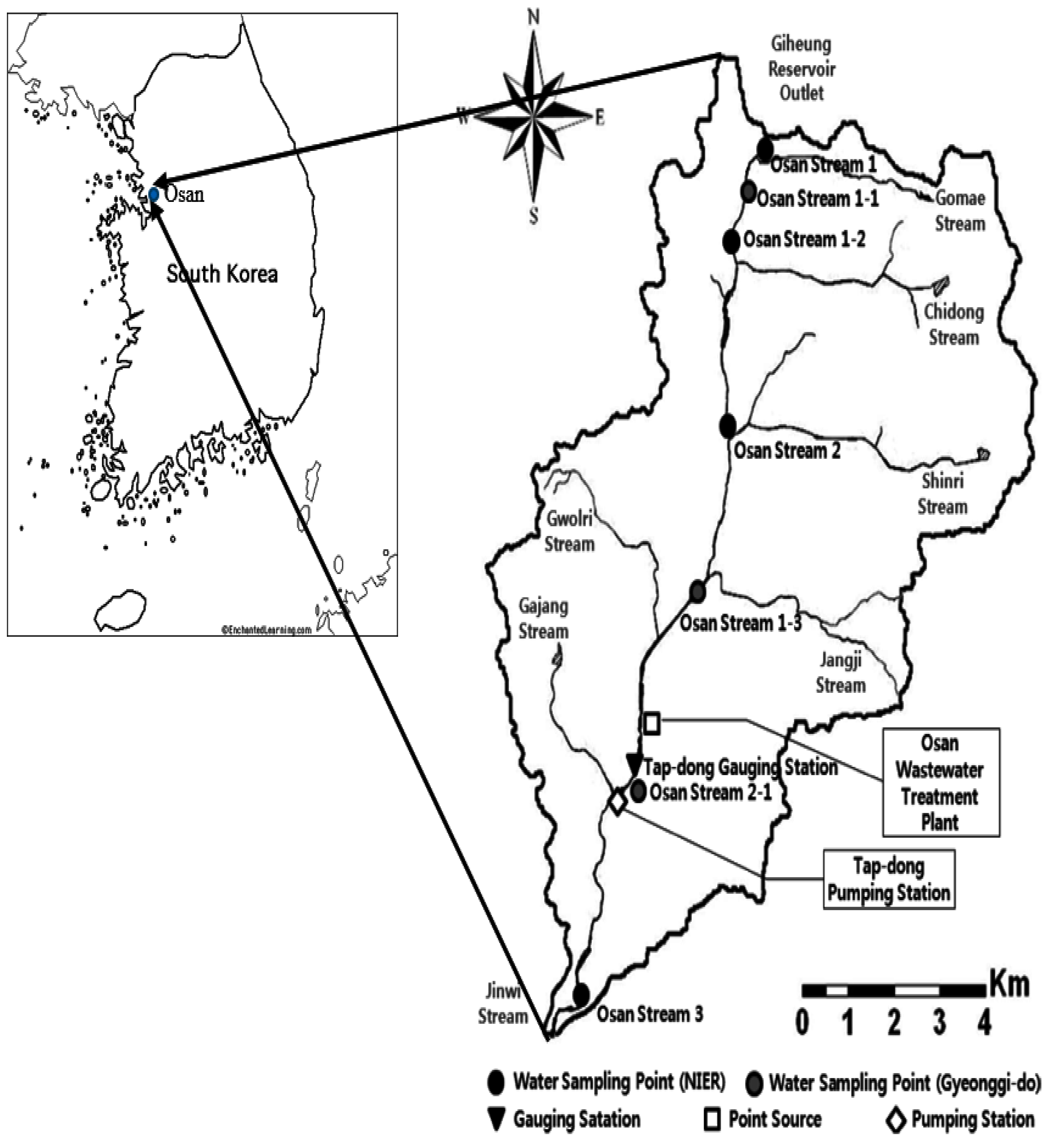
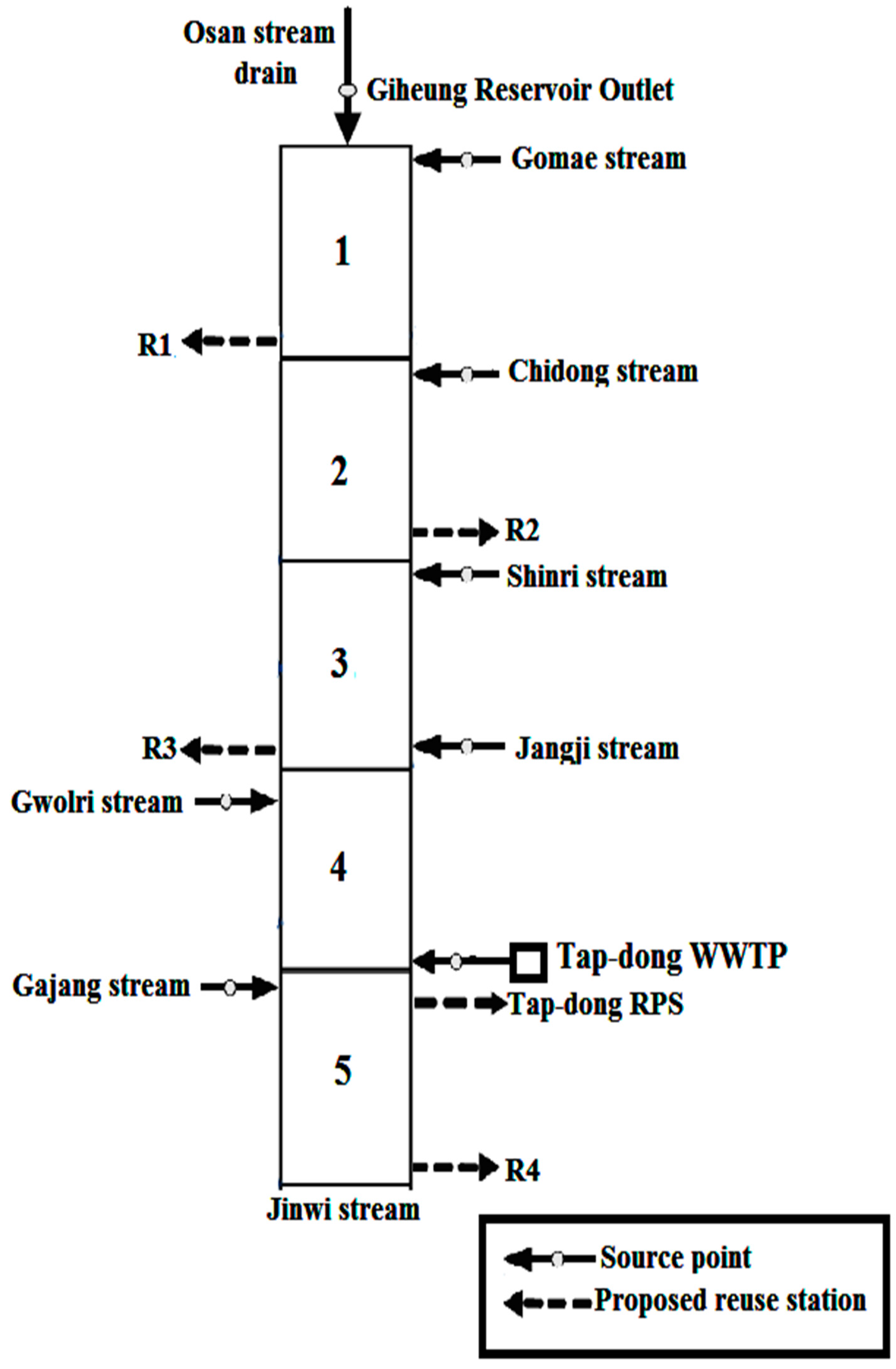
2. Study Area
3. Methods
3.1. Water Quality Modeling
3.1.1. Uncertainty Analysis
3.1.2. Sensitivity Analysis
3.2. Optimization of Drainage Water Reuse
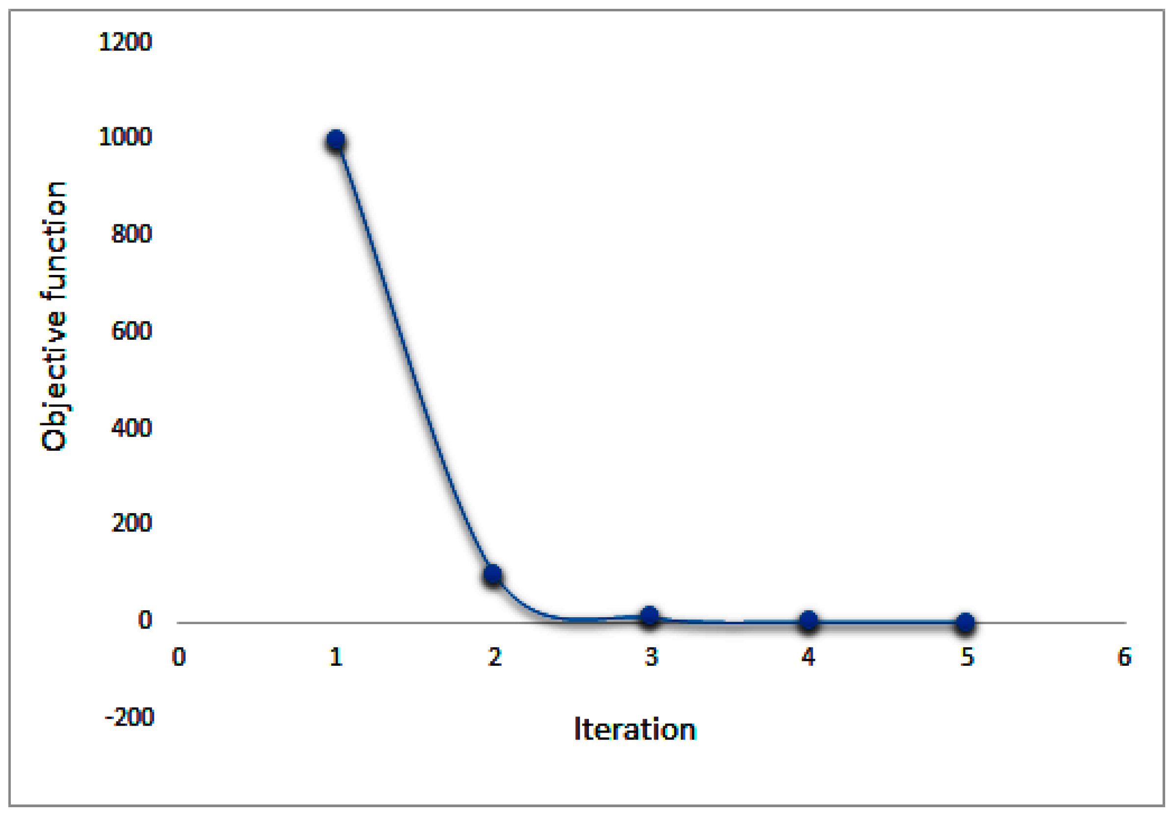
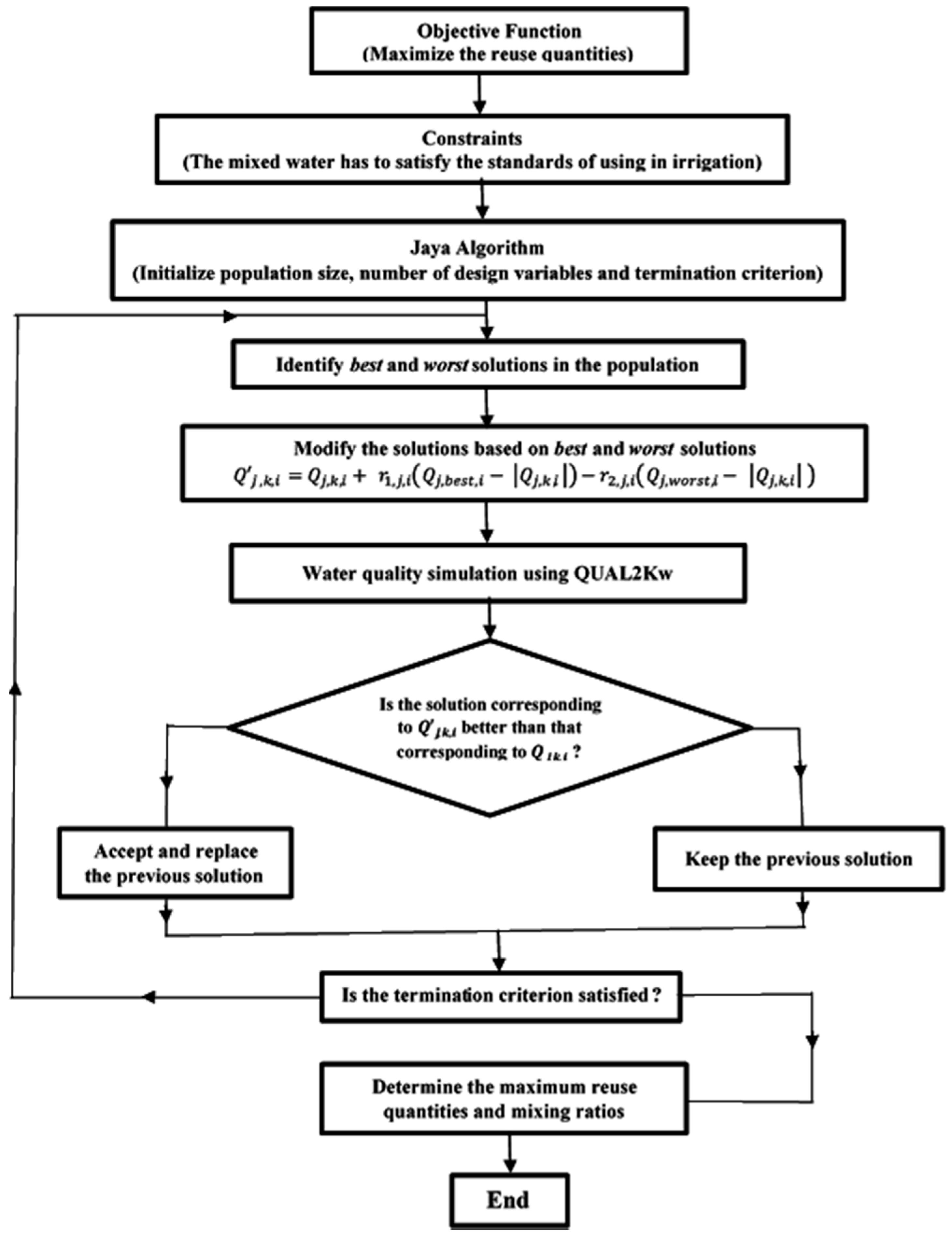
3.2.1. Jaya Algorithm
3.2.2. Jaya Algorithm Application
4. Results and Discussion
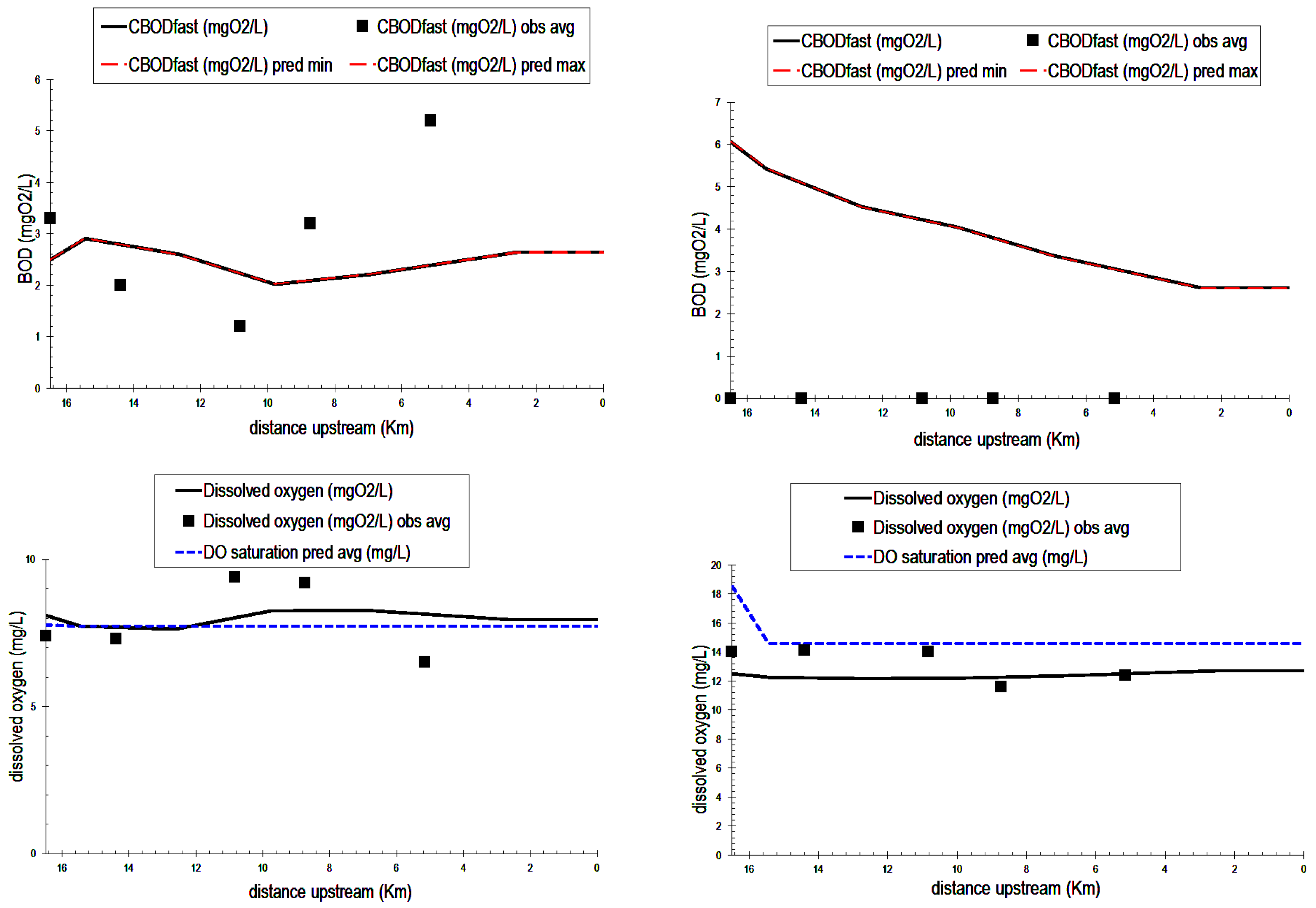
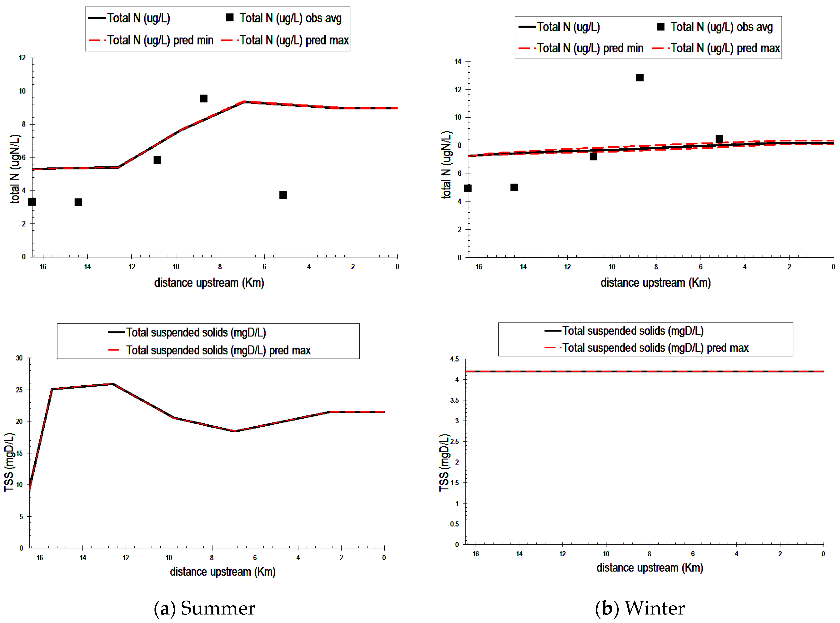
4.1. Water Quality Simulation
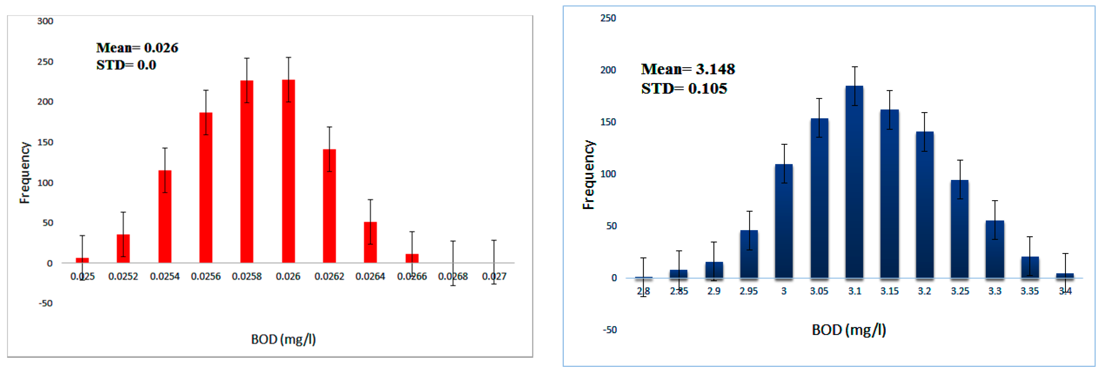
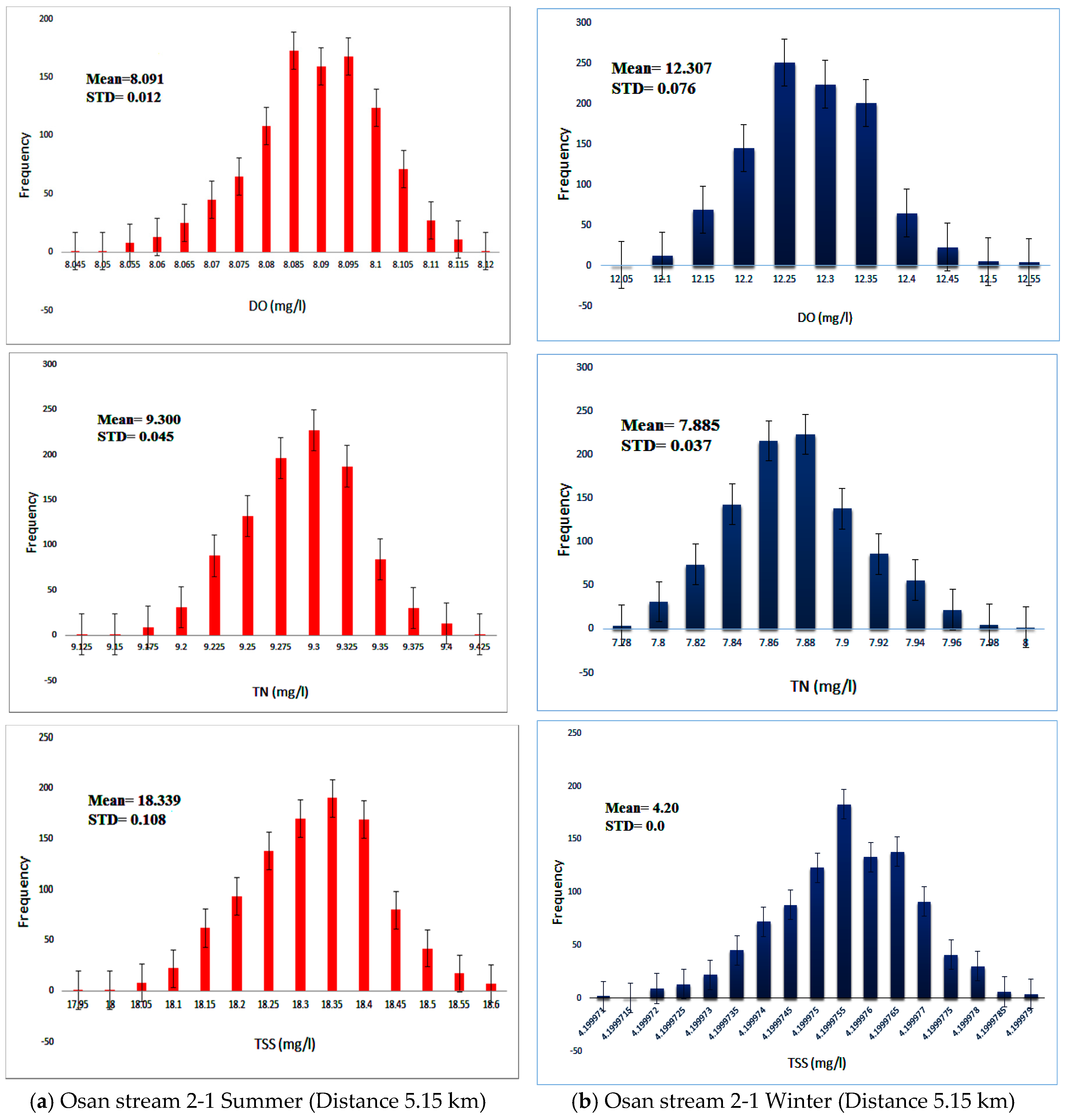
4.1.1. Uncertainty Analysis Outcome
4.1.2. Sensitivity Analysis Results
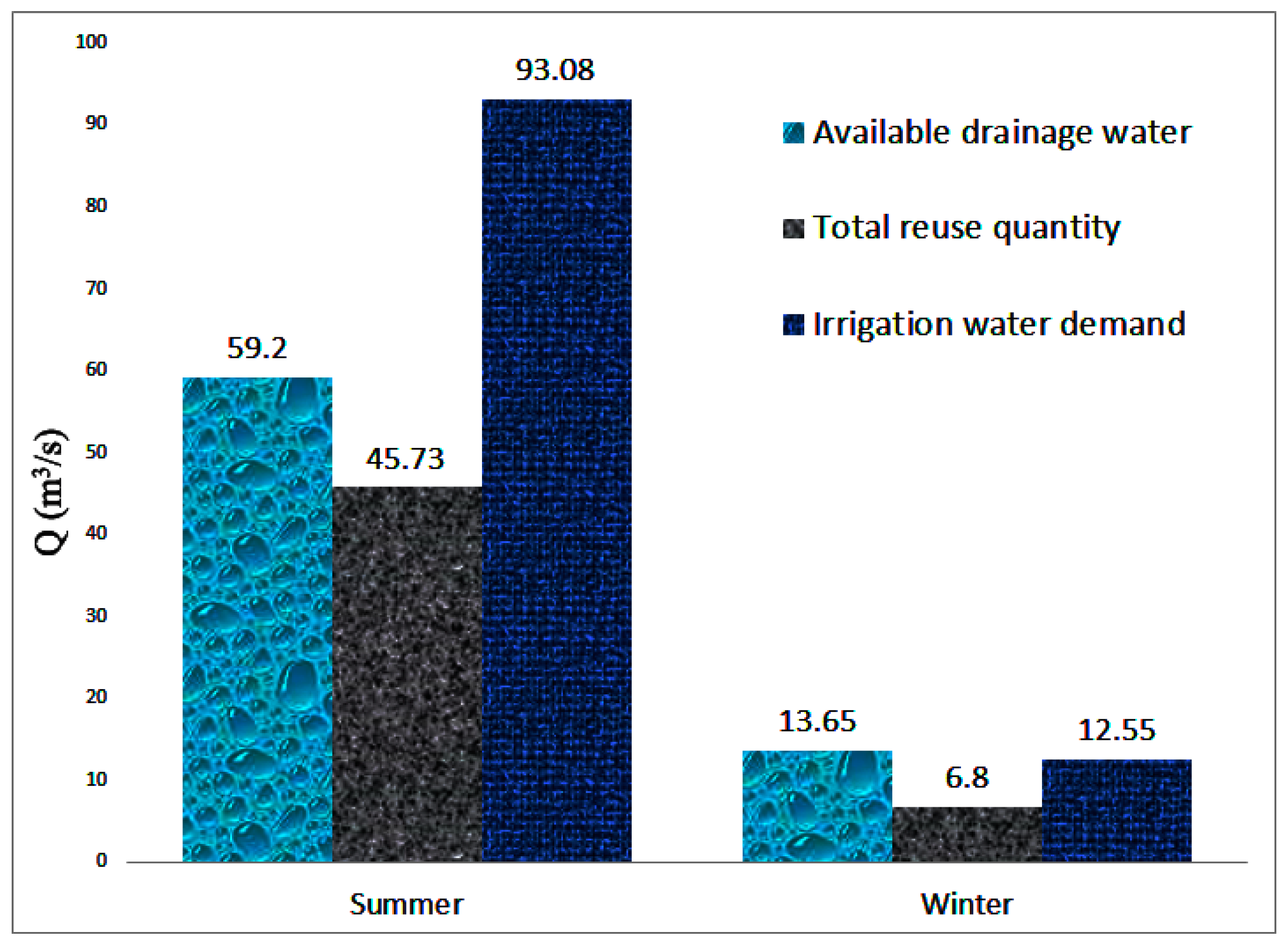
4.2. Optimization of ADW Reuse
5. Conclusions
Author Contributions
Funding
Conflicts of Interest
References
- FAO. Coping with Water Scarcity—Challenge of the Twenty-First Century; FAO: Rome, Italy, 2007. [Google Scholar]
- World Health Organization (WHO). Guidelines for the Safe Use of Wastewater, Excreta and Greywater, Volume 2: Wastewater Use in Agriculture; World Health Organization: Geneva, Switzerland, 2006. [Google Scholar]
- Hamilton, A.J.; Stagnitti, F.; Xiong, X.; Kreidil, S.L.; Benke, K.K.; Maher, P. Wastewater irrigation: The state of play. Vadose Zone J. 2007, 6, 823–840. [Google Scholar] [CrossRef]
- Ministry of Construction and Transportation. National Water Resource Plan; MOCT: Seoul, Korea, 2012. (In Korean)
- Ministry of Environment. Wastewater Reuse Guide Book; MOE: Seoul, Korea, 2009. (In Korean)
- Ministry of Land, Transportation and Maritime Affairs (MLTM). Water Vision 2020 (2006 National Water Resources Plan Update); MLTM: Seoul, Korea, 2006. (In Korean)
- Blumenthal, U.J.; Peasy, A.; Ruiz-Palacios, G.; Mara, D.D. Guidelines for Wastewater Reuse in Agriculture and Aquaculture: Recommended Revisions Based on New Research Evidence; WELL Study, Task No. 68 (Part 1); WELL Resource Centre: London, UK, 2000. [Google Scholar]
- Jeong, H.; Kim, H.; Jang, T.; Park, S. Assessing the effects of indirect wastewater reuse on paddy irrigation in the Osan River watershed in Korea using the SWAT model. Agric. Water Manag. 2016, 163, 393–402. [Google Scholar] [CrossRef]
- Kalburgi, P.; Shivayogimath, C.; Purandara, B. Application of QUAL2K for water quality modeling of river Ghataprabha (India). J. Environ. Sci. Eng. 2010, 4, 37. [Google Scholar]
- Vasudevan, M.; Nambi, I.; Suresh, K. Application of QUAL2K for assessing waste loading project in river Yamuna. Int. J. Adv. Eng. Technol. 2011, 2, 336–344. [Google Scholar]
- Gikas, G. Water quality of drainage canals and assessment of nutrient loads using QUAL2Kw. Environ. Process. 2014, 1, 369–385. [Google Scholar] [CrossRef]
- Fliefle, A.; Saavedraina, O.; Yoshimura, C.; Elzeir, M.; Tawfik, A. Optimization of integrated water quality management for agricultural efficiency and environmental conservation. Environ. Sci. Pollut. Res. 2014, 21, 8095–8111. [Google Scholar] [CrossRef] [PubMed]
- Allam, A.; Tawfik, A.; Yoshimura, C.; Fleifle, A. Simulation-based optimization framework for reuse of agricultural drainage water in irrigation. J. Environ. Manag. 2016, 172, 82–96. [Google Scholar] [CrossRef] [PubMed]
- Rashed, A.; El-Sayed, E. Simulating agricultural drainage water reuse using QUAL2K Model: Case study of the Ismailia canal catchment area. J. Irrig. Drain. Eng. 2014, 140, 501–511. [Google Scholar] [CrossRef]
- Song, J.H.; Jeong, H.S.; Park, J.H.; Song, I.H.; Kang, M.S.; Park, S.W. Analysis of water quality and soil environment in paddy fields partially irrigated with untreated wastewater. J. Korean Soc. Agric. Eng. 2014, 56, 19–29. [Google Scholar]
- American Public Health Association (APHA); American Water Works Association (AWWA); Water Environment Federation (WEF). Standard Methods for the Examination of Water and Wastewater, 20th ed.; United Book Press, Inc.: Baltimore, MD, USA, 1998. [Google Scholar]
- Ministry of Environment. Environmental Review 2011; MOE: Seoul, Korea, 2011. (In Korean)
- Brown, L.; Barnwell, T. The Enhanced Stream Water Quality Models QUAL2E and QUAL2E-UNCAS: Documentation and User Manual; Environmental Research Laboratory, Office of Research and Development, US Environmental Protection Agency: Athens, GA, USA, 1987.
- Pelletier, G. YASAI.xla: A Modified Version of an Open-Source Add-In for Excel to Provide Additional Functions for Monte Carlo Simulation; Department of Ecology: Washington, DC, USA, 2009. Available online: http://www.ecy.wa.gov/programs/eap/models.html (accessed on 1 January 2018).
- Models and Tools for Water Quality Improvement. Available online: https://ecology.wa.gov/Research-Data/Data-resources/Models-spreadsheets/Modeling-the-environment/Models-tools-for-TMDLs (accessed on 1 January 2017).
- Pelletier, G.; Chapra, S. A Modeling Framework for Simulating River and Stream Water Quality. QUAL2Kw Theory Documentation; 2005. Available online: http://www.ecy.wa.gov/programs/eap/models/ (accessed on 1 January 2018).
- Chapra, S.; Pelletier, G.; Tao, H. QUAL2K: A Modeling Framework for Simulating River and Stream Water Quality, Version 2.11: Documentation and User’s Manual; Civil and Environmental Engineering Department, Tufts University: Medford, MA, USA, 2008. [Google Scholar]
- Hye, K.J.; Seok, J.H.; Seong, K.M.; Hong, S.I.; Park, S.W. Simulation of 10-day Irrigation Water Quality Using SWAT-QUALKO2 Linkage Model. J. Korean Soc. Agric. Eng. 2012, 54, 53–63. [Google Scholar] [CrossRef] [Green Version]
- Caviness, K.; Garey, A.; Patrick, N. Modeling the Big Black River: A comparison of water quality models. J. Am. Water Resour. Assoc. 2006, 42, 617–627. [Google Scholar] [CrossRef]
- Paliwal, R.; Sharma, P.; Kansal, A. Water quality modelling of the river Yamuna (India) using QUAL2E-UNCAS. J. Environ. Manag. 2007, 2, 1–14. [Google Scholar] [CrossRef] [PubMed]
- Kim, H.D.; Lee, G.Y.; Lee, Y.G. Application of wastewater reuse system for agriculture: Status and prospects. Mag. Korea Water Resour. Assoc. 2009, 42, 36–43. (In Korean) [Google Scholar]
- Sharma, D.; Kansal, A.; Pelletier, G. Water quality modeling for urban reach of Yamuna River, India (1999–2009), using QUAL2Kw. Appl. Water Sci. 2015. [Google Scholar] [CrossRef]
- Eckstein, J.; Riedmueller, S.; Reed, S. YASAI: Yet Another Simulation Add-in for Excel. Version 2.0 User Guide. 2000. Available online: http://www.yasai.rutgers.edu/yasai-guide-20html (accessed on 1 January 2018).
- Eckstein, J.; Riedmueller, S. YASAI: Yet Another Add in for Teaching Elementary Monte Carlo Simulation in Excel; Rutcor Research Report (RRR) 27-2001, APRIL; Rutgers University: Piscataway, NJ, USA, 2001. [Google Scholar]
- Eckstein, J.; Riedmueller, S. YASAI: Yet another add in for teaching elementary Monte Carlo simulation in Excel. Inf. Trans. Educ. 2002, 2, 12–26. [Google Scholar] [CrossRef]
- Rao, R. Jaya: A simple and new optimization algorithm for solving constrained and unconstrained optimization problems. Int. J. Ind. Eng. Comput. 2016, 7, 19–34. [Google Scholar]
- Jang, T.; Lee, S.B.; Sung, C.H.; Lee, H.P.; Park, S.W. Safe application of reclaimed water reuse for agriculture in Kora. Paddy Water Environ. 2010, 8, 227–233. [Google Scholar] [CrossRef]
- Enforcement Decree of the Framework Act on Environmental Policy; Article 2, No. 23967; FAO: Rome, Italy, 2012. (In Korean)


| Monitoring Point | Distance (km) | pH | DO (mg/L) | BOD (mg/L) | COD (mg/L) | TSS (mg/L) | TN (mg/L) | TP (mg/L) | TOC (mg/L) | NH4-N (mg/L) | NO3-N (mg/L) |
|---|---|---|---|---|---|---|---|---|---|---|---|
| Osan stream 1 | 15.59 | 7.9 | 10.2 | 2.4 | 7.6 | 5.6 | 4.131 | 0.062 | 6.9 | 0.35 | 2.452 |
| Osan stream 1-2 | 14.39 | 7.7 | 10 | 2.8 | 7.4 | 22 | 4.72 | 0.071 | 6.8 | 0.227 | 2.578 |
| Osan stream 1-3 | 10.83 | 8 | 11.7 | 1.5 | 5.1 | 9.7 | 6.145 | 0.353 | 3.5 | 0.221 | 4.411 |
| Osan stream 2 | 8.73 | 7.8 | 10.4 | 1.6 | 6.3 | 17 | 4.212 | 0.117 | 5.7 | 0.134 | 2.691 |
| Osan stream 2-1 | 5.15 | 7.8 | 10.8 | 4.7 | 7.7 | 7.5 | 9.108 | 0.64 | 5.6 | 3.038 | 5.27 |
| Osan stream 3 | 0.49 | 7.6 | 9.3 | 6.4 | 8.8 | 24.1 | 6.43 | 0.316 | 8 | 1.15 | 2.869 |
| Proposed Reused Station | Location | Summer 2016 | Winter 2016 | ||||||
|---|---|---|---|---|---|---|---|---|---|
| BOD | DO | TSS | TN | BOD | DO | TSS | TN | ||
| (km) | (mg/L) | (mg/L) | (mg/L) | (mg/L) | (mg/L) | (mg/L) | (mg/L) | (mg/L) | |
| R1 | 14.36 | 3.3 | 7.4 | 39.8 | 3.4 | 2.2 | 12.5 | 4.2 | 6.1 |
| R2 | 10.81 | 2 | 7.3 | 27.5 | 3.3 | 1.2 | 13.4 | 6.5 | 5.1 |
| R3 | 8.60 | 1.2 | 9.4 | 11.3 | 6.1 | 1.8 | 13.9 | 8 | 6.3 |
| Tap-dong | 5.15 | 3.2 | 9.4 | 7.5 | 9.5 | 6.1 | 12.4 | 7.5 | 11.7 |
| R4 | 0.49 | 5.2 | 6.6 | 38.8 | 3.8 | 7.6 | 11.9 | 9.4 | 9.1 |
| Parameter | Adopted Values | Units | Minimum Values | Maximum Values |
|---|---|---|---|---|
| Carbon | 40 | gC | 30 | 60 |
| Nitrogen | 7.2 | gN | 5 | 9 |
| Phosphorus | 1 | gP | 0.5 | 2 |
| Dry weight | 100 | gD | 100 | 100 |
| Chlorophyll-a | 1 | gA | 0.5 | 2 |
| Slow CBOD hydrolysis rate | 0.11218 | /day | 0.05 | 0.25 |
| Slow CBOD oxidation rate | 3.89645 | /day | 0 | 5 |
| Fast CBOD oxidation rate | 0.0256 | /day | 0 | 5 |
| Organic N hydrolysis | 0.2304025 | /day | 0.05 | 0.3 |
| Organic N settling velocity | 0.534848 | m/day | 0.05 | 2 |
| Ammonium nitrification | 0.269893 | /day | 0.05 | 3 |
| Nitrate de-nitrification | 0.67172 | /day | 0 | 2 |
| Sediment de-nitrification transfer coefficient | 0.31265 | m/day | 0 | 1 |
| Organic P hydrolysis | 0.29292 | /day | 0.05 | 0.3 |
| Organic P settling velocity | 0.684998 | m/day | 0.05 | 2 |
| Inorganic P settling velocity | 0.9685 | m/day | 0 | 2 |
| Sediment P oxygen attenuation half saturation constant | 0.59594 | mgO2/L | 0 | 2 |
| Bottom Algae: | ||||
| Max growth rate | 157.1435 | mgA/m2/day or/day | 50 | 200 |
| Respiration rate | 0.48434 | /day | 0.02 | 0.2 |
| Excretion rate | 0.21083 | /day | 0 | 0.5 |
| Death rate | 0.096155 | /day | 0 | 0.5 |
| External nitrogen half sat constant | 497.36 | μgN/L | 100 | 500 |
| External phosphorus half sat constant | 35.51275 | μgP/L | 25 | 100 |
| Light constant | 61.1134 | langleys/day | 40 | 110 |
| Ammonia preference | 29.1867 | μgN/L | 15 | 30 |
| Subsistence quota for nitrogen | 15.054912 | mgN/mgA | 7.2 | 36 |
| Subsistence quota for phosphorus | 4.59572 | mgP/mgA | 1 | 5 |
| Maximum uptake rate for nitrogen | 1042.0815 | mgN/mgA/day | 350 | 1500 |
| Maximum uptake rate for phosphorus | 162.9995 | mgP/mgA/day | 50 | 200 |
| Internal nitrogen half sat ratio | 4.535006 | Dimensionless | 1.05 | 5 |
| BOD (mg/L) | DO (mg/L) | TSS (mg/L) | TN (mg/L) | |||||
|---|---|---|---|---|---|---|---|---|
| Summer | Winter | Summer | Winter | Summer | Winter | Summer | Winter | |
| Osan Stream 2-1 | ||||||||
| Mean | 0.026 | 3.148 | 8.091 | 12.307 | 18.345 | 4.2 | 9.302 | 7.885 |
| Minimum | 0.025 | 2.839 | 8.05 | 12.089 | 17.968 | 4.199 | 9.146 | 7.786 |
| Maximum | 0.027 | 3.424 | 8.121 | 12.592 | 18.649 | 4.2 | 9.427 | 8.017 |
| Range | 0.002 | 0.585 | 0.071 | 0.503 | 0.681 | 0.001 | 0.281 | 0.231 |
| Standard deviation | 0 | 0.105 | 0.012 | 0.076 | 0.105 | 0 | 0.012 | 0.037 |
| Coefficient of variation | 0 | 0.033 | 0.001 | 0.006 | 0.005 | 0 | 0.001 | 0.004 |
| Skewness Coefficient | 0.026 | −0.004 | −0.349 | 0.194 | −0.204 | −0.273 | −0.23 | 0.259 |
| Osan Stream 3 | ||||||||
| Mean | 0.038 | 2.375 | 7.74 | 12.66 | 21.344 | 4.2 | 8.922 | 8.179 |
| Minimum | 0.037 | 2.054 | 7.694 | 12.433 | 20.911 | 4.199 | 8.805 | 8.037 |
| Maximum | 0.039 | 2.673 | 7.771 | 12.94 | 21.69 | 4.2 | 9.013 | 8.369 |
| Range | 0.002 | 0.619 | 0.077 | 0.507 | 0.779 | 0.001 | 0.208 | 0.332 |
| Standard deviation | 0 | 0.111 | 0.012 | 0.081 | 0.12 | 0 | 0.033 | 0.053 |
| Coefficient of variation | 0 | 0.047 | 0.002 | 0.006 | 0.005 | 0 | 0.004 | 0.006 |
| Skewness Coefficient | −0.002 | 0.034 | −0.383 | 0.138 | −0.216 | −0.275 | −0.238 | 0.26 |
| Results for Summer | ||||||||||||||||
| Proposed Reused Station | Drain Water Upstream Mixing Point | Canal Water Upstream Mixing Point | Canal Water Downstream Mixing Points | |||||||||||||
| Qd,j | Qr,j | BOD | DO | TSS | TN | Qc,j | BOD | DO | TSS | TN | Q′r,j | BOD | DO | TSS | TN | |
| (m/s3) | (m/s3) | (mg/L) | (mg/L) | (mg/L) | (mg/L) | (m/s3) | (mg/L) | (mg/L) | (mg/L) | (mg/L) | (m/s3) | (mg/L) | (mg/L) | (mg/L) | (mg/L) | |
| R1 | 1.85 | 3.90 | 2.91 | 7.73 | 25.09 | 5.34 | 4.01 | 2.51 | 6.91 | 22.23 | 3.65 | 7.91 | 4.12 | 7.58 | 23.59 | 3.89 |
| R2 | 1.85 | 5.92 | 2.59 | 7.63 | 25.92 | 5.38 | 5.98 | 2.15 | 6.74 | 21.56 | 3.25 | 11.9 | 3.95 | 6.99 | 22.99 | 4.10 |
| R3 | 1.85 | 9.95 | 2.03 | 8.25 | 19.99 | 7.64 | 10.56 | 1.87 | 7.15 | 16.58 | 5.98 | 20.51 | 2.56 | 7.89 | 17.23 | 6.65 |
| Tap-dong | 1.85 | 11.97 | 2.22 | 8.28 | 17.88 | 9.34 | 12.21 | 2.02 | 7.09 | 15.67 | 7.59 | 24.18 | 3.22 | 7.58 | 16.48 | 8.49 |
| R4 | 1.85 | 13.99 | 2.64 | 7.94 | 20.90 | 9.85 | 14.59 | 2.05 | 7.01 | 18.12 | 8.11 | 28.58 | 3.01 | 7.25 | 19.56 | 9.03 |
| 45.73 | 47.35 | 93.08 | ||||||||||||||
| Results for winter | ||||||||||||||||
| Proposed Reused Station | Drain Water Upstream Mixing Point | Canal Water Upstream Mixing Point | Canal Water Downstream Mixing Points | |||||||||||||
| Qd,j | Qr,j | BOD | DO | TSS | TN | Qc,j | BOD | DO | TSS | TN | Q′r,j | BOD | DO | TSS | TN | |
| (m/s3) | (m/s3) | (mg/L) | (mg/L) | (mg/L) | (mg/L) | (m/s3) | (mg/L) | (mg/L) | (mg/L) | (mg/L) | (m/s3) | (mg/L) | (mg/L) | (mg/L) | (mg/L) | |
| R1 | 1.34 | 1.36 | 5.43 | 12.26 | 4.20 | 7.35 | 1.15 | 4.95 | 10.95 | 2.96 | 5.94 | 2.51 | 4.99 | 11.23 | 3.02 | 6.25 |
| R2 | 1.34 | 1.36 | 4.52 | 12.18 | 4.20 | 7.56 | 1.15 | 4.01 | 10.84 | 2.86 | 6.35 | 2.51 | 4.23 | 11.06 | 3.11 | 6.98 |
| R3 | 1.34 | 1.36 | 4.04 | 12.20 | 4.20 | 7.68 | 1.15 | 3.26 | 10.21 | 2.52 | 6.38 | 2.51 | 3.56 | 10.89 | 2.88 | 7.41 |
| Tap-dong | 1.34 | 1.36 | 3.36 | 12.37 | 4.20 | 7.88 | 1.15 | 2.42 | 9.97 | 3.52 | 5.84 | 2.51 | 2.68 | 10.13 | 3.95 | 6.68 |
| R4 | 1.34 | 1.36 | 2.61 | 12.69 | 4.20 | 8.17 | 1.15 | 1.96 | 11.02 | 3.86 | 6.72 | 2.51 | 2.12 | 12.11 | 4.00 | 7.25 |
| 6.80 | 5.75 | 12.55 | ||||||||||||||
© 2018 by the authors. Licensee MDPI, Basel, Switzerland. This article is an open access article distributed under the terms and conditions of the Creative Commons Attribution (CC BY) license (http://creativecommons.org/licenses/by/4.0/).
Share and Cite
Ashu, A.; Lee, S.-I. Reuse of Agriculture Drainage Water in a Mixed Land-Use Watershed. Agronomy 2019, 9, 6. https://doi.org/10.3390/agronomy9010006
Ashu A, Lee S-I. Reuse of Agriculture Drainage Water in a Mixed Land-Use Watershed. Agronomy. 2019; 9(1):6. https://doi.org/10.3390/agronomy9010006
Chicago/Turabian StyleAshu, Agbortoko, and Sang-Il Lee. 2019. "Reuse of Agriculture Drainage Water in a Mixed Land-Use Watershed" Agronomy 9, no. 1: 6. https://doi.org/10.3390/agronomy9010006
APA StyleAshu, A., & Lee, S.-I. (2019). Reuse of Agriculture Drainage Water in a Mixed Land-Use Watershed. Agronomy, 9(1), 6. https://doi.org/10.3390/agronomy9010006