Technical Note

The Prognostic Breeding Application JMP Add-In Program

1
Institute of Plant Breeding, Genetics & Genomics and Dept. of Crop and Soil Sciences, University of Georgia, 111 Riverbend Road, Athens, GA 30602, USA
2
Agricultural Statistics Laboratory, University of Arkansas, Fayetteville, AR 72701, USA
*
Author to whom correspondence should be addressed.
Agronomy 2019, 9(1), 25; https://doi.org/10.3390/agronomy9010025
Submission received: 4 December 2018 / Revised: 3 January 2019 / Accepted: 7 January 2019 / Published: 9 January 2019

Abstract

:
Prognostic breeding is a crop improvement methodology that utilizes prognostic equations to enable concurrent selection for plant yield potential and stability of performance. There is a necessity for plant breeders to accurately phenotype plants in the field and select effectively for high and stable crop yield in the absence of the confounding effects of competition. Prognostic breeding accomplishes this goal by evaluating plants for (i) plant yield potential and (ii) plant stability, in the same generation. The plant yield index, stability index and the plant prognostic equation are the main criteria used for the selection of the best plants and the best entries grown in honeycomb designs. The construction of honeycomb designs and analysis of experimental data in prognostic breeding necessitate the development of a computer program to ensure accurate measurement of the prognostic equations. The objective of this paper is to introduce the Prognostic Breeding Application JMP Add-In, a program for constructing honeycomb designs and analyzing data for the efficient selection of superior plants and lines. The program displays powerful controls, allowing the user to create maps of any honeycomb design and visualize the selected plants in the field. Multi-year soybean data are used to demonstrate key features and graphic views of the most important steps.

1. Introduction

To meet the challenges of genetic improvement, new efficiencies in breeding should be introduced to accelerate the progress through selection and maximize the annual genetic gain [1]. Prognostic breeding is a crop improvement methodology that utilizes the honeycomb selection designs and the prognostic equations to enable concurrent selection for plant yield potential and stability of performance [2]. The unit of evaluation and selection in prognostic breeding is the single plant grown in the absence of interplant competition for reasons that have been discussed expensively by Fasoula and Fasoula [3,4,5]. The range of phenotypic expression is maximized because plants express their full genetic potential for tillering capacity and robust root systems [3,4,5,6,7]. Additional details on the principles of this methodology are discussed in the following review papers [2,3,4,5,8,9].
There is a necessity for plant breeders to accurately phenotype plants in the field and select effectively for both plant yield potential and stability of performance. Prognostic breeding accomplishes this goal by evaluating plants for the two components of the crop yield potential: (1) plant yield potential (using the plant yield index) and (2) plant stability (using the stability index), measured in the same generation [2]. Accurate measurement of the above parameters is accomplished by using the unique features of honeycomb designs [8].
Honeycomb selection designs are advanced experimental designs that possess some innovative properties. They utilize moving circular replicates/rings to ensure increased local control and moving triangular grids to ensure effective sampling for soil heterogeneity [8]. In any honeycomb design, each plant is located in the center of a moving replicate/ring. This permits effective reduction of the masking effects of soil heterogeneity by using the plant yield index (PI). The designs allocate plants of each entry in a moving triangular grid spreading across the whole field, sampling effectively for soil heterogeneity. Formation of moving grids allows proficient measurement of stability of performance by using the stability index (SI). The product of PI and SI gives the plant prognostic equation (PPE) which measures the crop yield potential of each plant and is used for the selection of superior plants [2,10,11].
The prognostic breeding methodology speeds up the early stages of plant selection, reduces the time-frame required to release cultivars, and accelerates the genetic improvement of crops [2]. It utilizes high selection pressures in order to increase selection efficiency and maximize the annual genetic gain. When this methodology was applied in maize (Zea Mays L.) for 5 cycles, it produced an average annual genetic gain that ranged from 23% to 36%, providing evidence that selection efficiency can be significantly maximized and progress through selection can be accelerated [12].
The objective of this work is to introduce a JMP Add-In program as a useful tool for the construction of the different honeycomb designs and the analysis of data in order to select effectively the best entries and the best plants per entry. This software represents a powerful upgrade from the previous version developed by Mauromoustakos et al. [13]. The software is exemplified by using multi-year soybean data to demonstrate the construction of unreplicated and replicated designs along with graphic views of the most important steps.
The Prognostic Breeding Application is a JMP Add-In, a program for constructing honeycomb designs and analyzing data for the efficient selection of superior plants and lines. It was presented at JMP Discovery Summit Europe 2018 in Frankfurt by Mauromoustakos et al. [14].

2. Materials and Methods

2.1. Honeycomb Designs and Prognostic Equations Used to Select for High and Stable Crop Yield Potential

Honeycomb designs [8] are used in the prognostic breeding methodology of crop improvement [2]. They can be unreplicated or replicated and can accommodate a large number of plants in various crops, ranging from inbreeders to outbreeders to clonally propagated crops [2,4,8]. In unreplicated designs, each plant is its own entry.
Replicated designs include multiple plants for each entry. They are systematic designs possessing some innovative properties, the most important ones being: i) the formation of moving replicate/rings and ii) the formation of moving triangular grids [2,8]. Replicated designs use moving rings to minimize the masking effects of soil heterogeneity on single-plant yields and moving triangular grids to ensure effective sampling of field heterogeneity, essential for comprehensive selection of stability. Due to the formation of moving rings and moving grids, replicated designs are only available for a selected number of entries (Figure 1).
The possible number of entries (R) allowable in replicated honeycomb designs is given by the formula R = X2 + XY + Y2, where X and Y are integer numbers [2,8]. A partial list of replicated honeycomb designs, obtained when the X and Y take values from 0 to 9, is depicted in Figure 1. The numbers in the center of the squares are the allowable number, R, of entries. For example, the Replicated-3 (X = 1, Y = 1) honeycomb design evaluates 3 entries, while the Replicated-109 (X = 5, Y = 7) honeycomb design evaluates 109 entries. The construction of any replicated honeycomb design requires identification of the starting number of each field row through a parameter K. The numbers in the corners of squares represent the K numbers, which are used for the identification of the starting numbers of each row [8].
For every honeycomb design, the starting numbers of each field row are unique and are specified by the parameter K. Honeycomb designs have two or four Ks (Figure 1), meaning that there simply are two or four ways to construct the same design. Different Ks produce different starting numbers of field rows and therefore, different arrangements of entries in the field. Details on the construction of the designs are discussed in Fasoulas and Fasoula [8].
Figure 2 displays the arrangement of 21 entries of a Replicated-21 honeycomb design constructed using the parameters X = 1, Y = 4 and K = 4. The innovative features of the honeycomb designs, i.e., the formation of moving replicate/rings and moving triangular grids will be demonstrated by using as an example this design.
Honeycomb designs ensure that every plant lies in the center of a complete moving replicate/ring. As Figure 2 shows, each plant is placed in the center of a moving replicate/ring, shown for two random plants of line no. 9 (green circles). Thus, each plant is always surrounded by plants that belong to the same lines. The plant yield index P I = ( x / x ¯ r ) 2 measures plant yield devoid of the confounding effects of soil heterogeneity, because x is the yield of each plant and x ¯ r is the mean yield of the surrounding plants within the specified moving ring [2,10,11].
In our example, the moving ring consists of 18 plants (green circles). It is important to note that the size of the moving ring can vary; the smallest ring size is 6 plants and the largest ring size can include more than 120 plants [4,8]. No matter the size of the moving ring, each plant is always surrounded by moving-ring plants that belong to the same lines (entries). The choice of the size of the moving ring depends on the genetic structure and size of the population being sampled and on the degree of soil homogeneity.
Formation of moving replicates/rings ensure that plants of each line are placed in the corners of a moving triangular grid (shown here for line no. 9) which ensures effective sampling of soil heterogeneity and allows measurement of the stability index S I = ( x ¯ g / s ) 2 [2,10,11]. In the SI formula, x ¯ g and s denote the mean plant yield and standard deviation, respectively, of the line’s plants laid out in a moving grid. The moving grids are formed for the plants of each line and for every honeycomb design.
The product of the PI and SI gives the Plant Prognostic Equation (PPE) which measures the crop yield potential of each plant and is used for the selection of best plants [2,10,11].
P P E = ( x / x ¯ r ) 2 · ( x ¯ g / s ) 2
In addition to the PPE, the Line Prognostic Equation (LPE) can be used for the selection of the best lines [2,11].
L P E = ( x ¯ g / x ¯ t ) 2 · ( x ¯ g / s ) 2
The LPE is the product of the Line yield index L I = ( x ¯ g / x ¯ t ) 2 and the stability index S I = ( x ¯ g / s ) 2 , where x ¯ t is the mean plant yield of the whole trial.
The MeanPPE (average PPE value for the line) and LPE produce similar results since they both measure concurrently yield potential and stability of performance. The user can decide which one to use. The PI, SI, LI, LPE and PPE are unitless. Their use speeds up the early stages of plant selection and accelerates the annual genetic gain by effectively increasing selection pressure to only keep the very best plants [2,12].
Honeycomb designs can be laid out in any field orientation, square or rectangular; to accommodate the specific needs of different plant breeding programs. Missing plants present no problem because they affect neither the yield of nearby plants due to the use of ultra-wide spacings nor the efficiency of selection due to the use of numerous plants within the moving ring. The PI and PPE for plants on the border are calculated with incomplete moving rings.

2.2. JMP Add-In Specifications

The Prognostic Breeding Application is a JMP Add-In that contains two programs: Honeycomb Design Selection and Honeycomb Analysis [14]. This application suite was developed under JMP Version 13.2.1 for Windows and requires installation of the JMP software. It has been tested under Windows and MacOS of JMP.
The Honeycomb Design Selection program constructs a JMP table for a specific honeycomb design corresponding to a specified number of entries, field rows and plants per row as presented by Mauromoustakos et al. [14]. The user runs the Honeycomb Design Selection program by selecting it from the JMP Add-Ins menu. When the user starts the Honeycomb Design Selection program, the Honeycomb design selection widow is displayed (Figure 3). The user can click on the Design list-box to select a honeycomb design corresponding to the number of entries in the experiment. Many designs have alternate arrangements of the entries. These alternatives may be selected by the Design K list-box. The design parameters for the selected design are displayed.
The Honeycomb Design Selection program can be used to generate replicated honeycomb designs with frequently used number of entries, an UN (unreplicated) design and a UN-1 (unreplicated with 1 check) design as shown in Fasoulas and Fasoula [8]. The user can click on the More designs button to update the Design list box to display additional honeycomb designs for different numbers of entries. The user can enter the number of rows in the field and the number of plants in each row and the distance between plants. The Create button generates the specified design.
The Honeycomb Analysis program displays a graphic view of a honeycomb design stored in a JMP table as shown by Mauromoustakos et al. [14]. The user may optionally color and label the points in the graph. The program can calculate Moving Ring averages corresponding to various Moving Ring sizes and summary tables for replicated designs.
If the data file is a JMP table originally created by the JMP program, the Honeycomb Analysis program is embedded within the JMP table as a table property. After opening the JMP table, the user can run the Honeycomb Analysis program by right-clicking on it in the table property area and selecting RunScript. Alternatively, the user can run the Honeycomb Analysis program by selecting it from the JMP Add-Ins menu.
The Honeycomb Analysis program requires that the X and Y axis columns correspond to the physical location of the plants within the field. The Honeycomb Analysis program displays a field map with the axes adjusted to emphasize the honeycomb pattern of the plants. The graph is a standard JMP Overlay Plot. The program displays powerful controls that allow the user to modify the graphs and visualize the data. The standard JMP controls are also available. The Honeycomb Analysis program makes extensive use of the Selection, Color and Label row states [14].
The Color plants control modifies the JMP table’s row state to color the graph points by the selected columns. Coloring by a continuous column colors the points in shades of blue, corresponding to the value of the column. Coloring by a nominal or ordinal column selects a different color based upon level of the column.
The Label plants control sets the Label property for the selected columns. Hovering the mouse over a point in the graph displays the values of these columns for these points.
The Select plants control emphasizes a subset of plants. The user may also select plants from the JMP table, a data filter, or the graph.
The Graph axes control provides an easy method to display a subset of the graph. The user may also modify the axis settings by right-clicking on the axis.
The Moving ring control allows the user to create moving ring variables for a selected continuous column using a moving ring of the specified size. If an Entry column is included, additional moving ring variables suitable for replicated designs are calculated. The moving ring variables include the response, entry and ring size as a part of the variable name [14].
For replicated designs, the program displays summary tables which calculate the PI, SI, LI, and the prognostic equations PPE and LPE used for the efficient selection of the best lines and the best plants per line. The PI, SI, LI, LPE and PPE are unitless indices allowing valuable comparisons of trials across years and locations. Their use speeds up early generation selection and increases annual genetic gain by effectively using high selection pressures (1–2%) to only keep the very best plants [2,12].

2.3. Data Material Used for the Case Study

Field studies in soybean (Glycine max L.) grown across years on agricultural land in the USA are used to illustrate the Prognostic Breeding Application for the construction and analysis of honeycomb designs and for the selection of best plants and lines. Over time, the performance of crop cultivars can deteriorate requiring the development of newer lines [2,3,4]. Elite gene pools have inherent mechanisms to provide a continuing source of new genetic variation [15]. Molecular data provide evidence that the genome is plastic, dynamic and constantly changing [16,17,18,19], and long-term selection experiments suggest that selection gain can be continual [20,21].
A multi-year program was implemented in order to develop improved lines of the soybean cultivar “Haskell” [2]. In the first cycle, plants from “Haskell” foundation seed were grown in an Unreplicated honeycomb design. Twenty best plants from this cycle were selected based on the Plant Index (PI) for Yield and formed the 20 candidate lines of the next cycle. In the second cycle, multiple plants from these 20 lines, plus foundation seed as the check line, were grown in a Replicated-21 honeycomb design. Based on the highest Plant Prognostic Equation (PPE) values, the best candidate lines and the best plants within these lines were selected for investigation in additional cycles.

3. Results and Discussion: Demonstrating the New JMP Add-In Program

Data from a multi-year experiment in soybean will be used to illustrate the use of the JMP Add-In program for the selection of superior plants and lines in soybean. This data is included in the JMP Add-In.

3.1. Cycle 1: Unreplicated Honeycomb Design—Construction, Data Analysis and Selection of Best Plants

Seeds were obtained from the Foundation seed source of the soybean cultivar “Haskell”. Seeds were planted in an Unreplicated honeycomb design that evaluated 420 plants in 30 rows and 14 plants per row, using a plant spacing of 0.9 m. After emergence, hill plots were thinned to contain a single plant. Plants were harvested when they reached maturity [2].
To construct the aforementioned unreplicated honeycomb design, the user can employ the following steps. From the JMP Add-Ins menu, select the Prognostic Breeding Application and go to the Honeycomb Design Selection item. In the Honeycomb Design Selection window, select the UN design from the Design drop-down box. The Field size control allows the user to specify the number of rows and plants per row in the field. Enter 14 in the Plants across box, 30 in the Rows down box and 0.9 in the Plant spacing box as shown in Figure 3.
Press the Create button when finished. This will create a JMP data table for the unreplicated honeycomb design with 30 rows and 14 plants per row. The XPosition and YPosition columns denote the placement of each plant in the field (Figure 4).
Record the traits of interest in the JMP data table. In this experiment we recorded seed yield (i.e., the seed yield of each plant). Columns may be renamed (i.e., Observation to YLD, Entry to PlantID) and additional columns may be created as desired. The data values in the Entry column may be modified but the columns Row, Plant, XPosition, YPosition should not be modified.
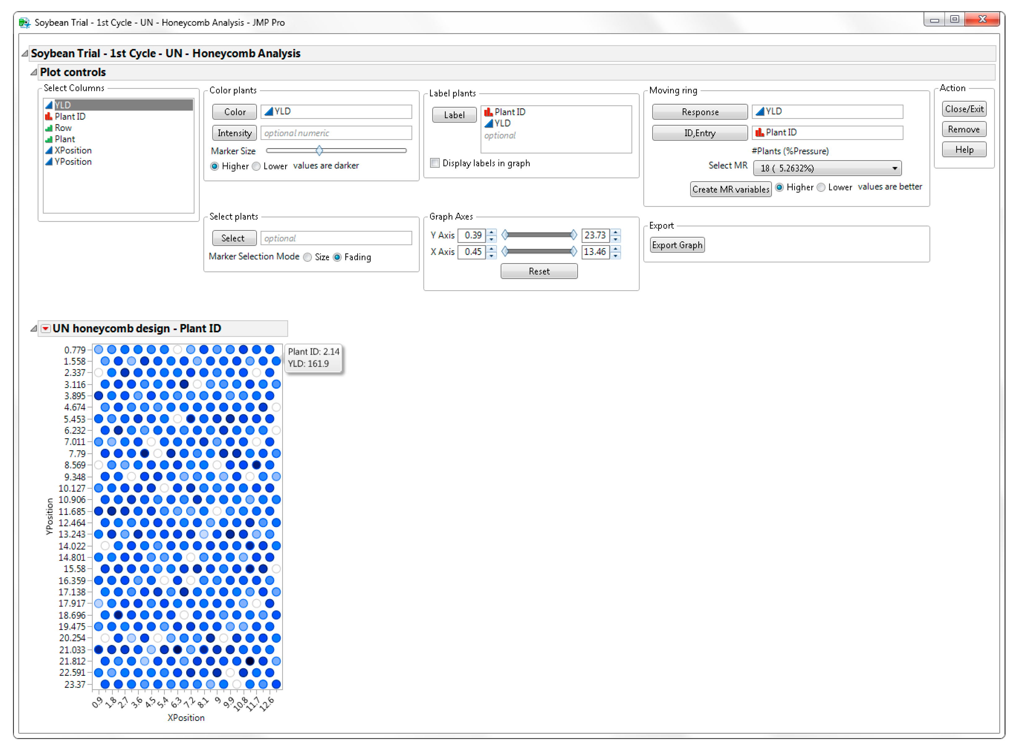
For the analysis, run the Honeycomb Analysis table script embedded within the JMP table. The program generates the graphic view of the design and Plot Controls that allow the user to visualize data points, analyze the data, and select plants as shown in Figure 5.
You can assign the column YLD to the Color role to color the graph according to the value of the yield to get an idea of the highest-yielding plants in this field. You can label plants by PlantID and YLD columns. In this case, hovering the mouse over a point in the graph displays the values of PlantID and YLD for these points, as shown for the last plant of row 2 in the honeycomb graph (Figure 5). Missing plants are displayed as white circles. Assign the column YLD to the Moving Ring Response role. Select the Moving Ring size. In this example, we selected a moving ring of 18 plants (MR = 18) (Figure 5). Press the Create MR variables button.
The necessary moving ring variables are added to the JMP table, so that the breeder can carry out the selection of plants. In the unreplicated honeycomb designs, selection of the best plants is performed based on the PI(YLD) column. The P I ( Y L D ) = ( x / x ¯ r ) 2 compares and adjusts the yield of each plant to the mean plant yield of its 18 surrounding moving-ring plants. We decided to select the best 20 plants.
To select the best 20 plants, assign the Rank PI column to the Select Plants role and adjust the selection limits to 1 and 20. Since one of the selected plants is on the border, you can decide to keep the border plant which has been evaluated with a smaller moving ring size, or you can increase the selection limit until 20 non-border plants are selected. We decided to drop the border plant, thus we assigned the selection limits to 1 and 21 in order to select 20 non-border plants (Figure 6). From the JMP menu, select Tables and go to Subset to create a JMP table of the selected plants.
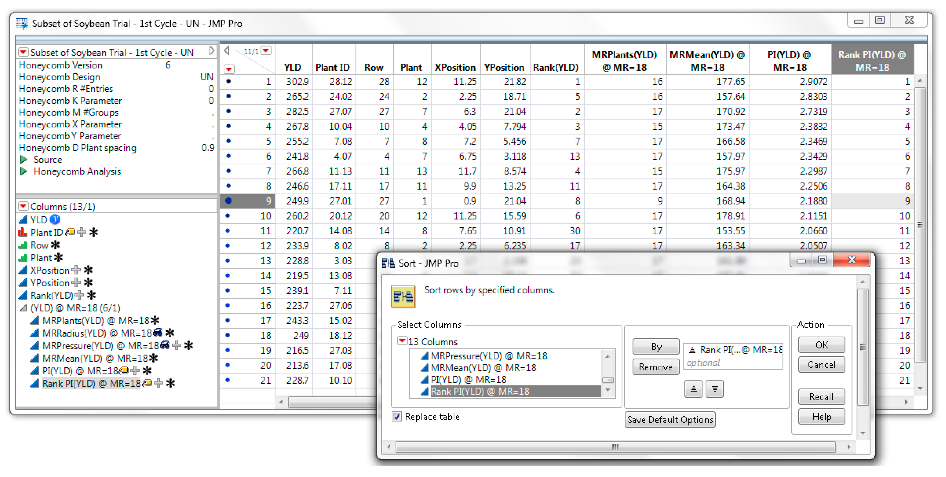
This creates a subset of the JMP table that contains only the 21 selected plants as shown in Figure 7. You can sort the subset JMP table by Rank PI(YLD). Delete the border plant (Plant = 1, Row = 27) from the subset. Save this JMP table for future reference. As the data show, when a moving ring of 18 plants was used (MR = 18), the best 20 plants had a PI(YLD) > 1.77, while the two highest-ranking plants had a PI(YLD) value of 2.91 and 2.83, respectively.
The PI(YLD), and therefore the best plants, depends upon the moving ring size selected. The breeder may calculate the PI(YLD) for different moving ring sizes (i.e., MR = 18 plants and MR = 30 plants) by changing the moving ring size and pressing the Create MR variables button. The size of the moving ring depends on the genetic structure and size of the population being sampled and on the degree of soil homogeneity [4,8]. Heterogeneous fields require smaller moving ring sizes than homogeneous fields. After comparing the PI(YLD) for different moving ring sizes, the breeder may decide to modify his/her choice of which plants are “best.”

3.2. Cycle 2: Replicated Honeycomb Design—Construction, Data Analysis and Selection of Best Lines and Best Plants

Seeds from the 20 best plants (from cycle 1) plus the check were planted in a Replicated-21 honeycomb design (Figure 2). Each of these selected plants forms a candidate line. Foundation seed from “Haskell” was assigned to the 21st line (representing the check). The seeds were planted in a R-21 honeycomb design of 672 plants in 14 rows, 48 plants per row, using a plant spacing of 0.9 m [
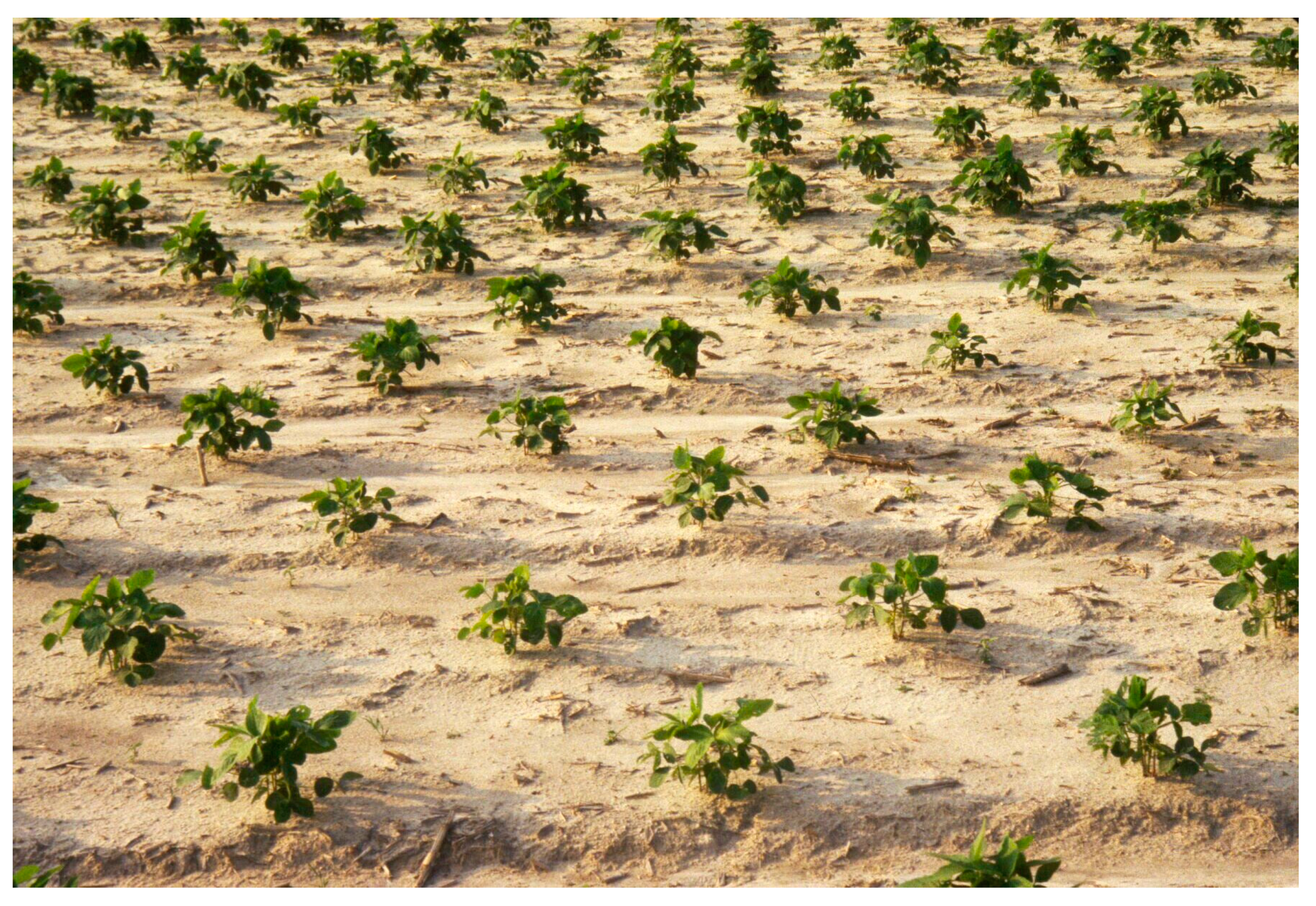
2]. There were 32 plants for each line. After emergence, hill plots were thinned to contain a single plant. Plants were harvested when they reached maturity. A partial view of the soybean experiment is depicted in Figure 8. While a square arrangement of plants produces field rows and alleys in two directions, a triangular arrangement of plants produces field rows and alleys in three directions (Figure 8).
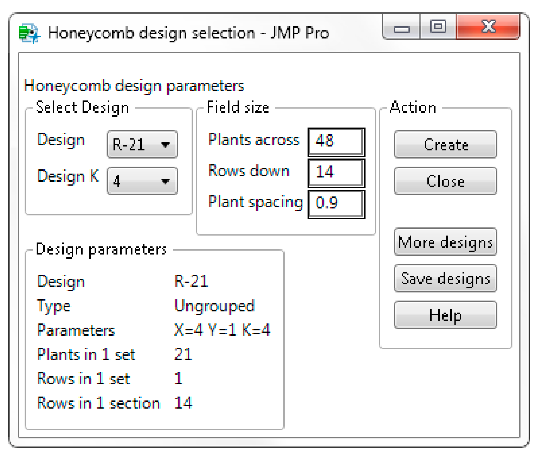
To construct the aforementioned replicated honeycomb design the user can employ the following steps. From the JMP Add-Ins menu, select the Prognostic Breeding Application and go to Honeycomb Design Selection item. Select R-21 in the Design box and 4 in the Design K box. If you select 16 in the Design K box, the R-21 will be constructed with an alternative arrangement of entries. Enter 48 in the Plants across box, 14 in the Rows down box and 0.9 in the Plant spacing box as shown in Figure 9.
Press the 
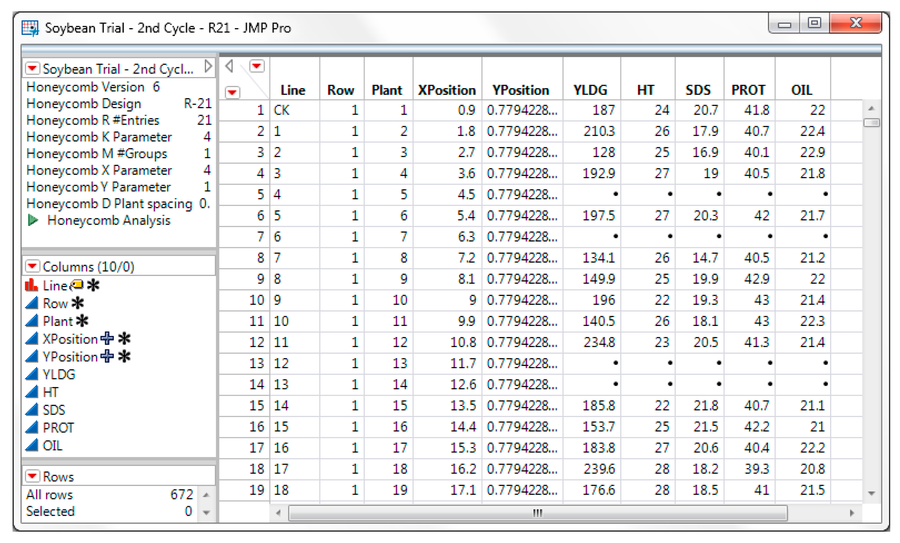
Create button to create the JMP table (Figure 10). Record the traits of interest in the JMP data table. In this experiment we recorded Seed yield (YLDG), Height (HT), Seed size (SDS), Seed protein (PROT) and Seed oil (OIL) as shown in Figure 10. The Entry column was renamed and JMP values labels were used to identify the check. The columns Row, Plant, XPosition, YPosition should not be modified.
To analyze the data, run the 
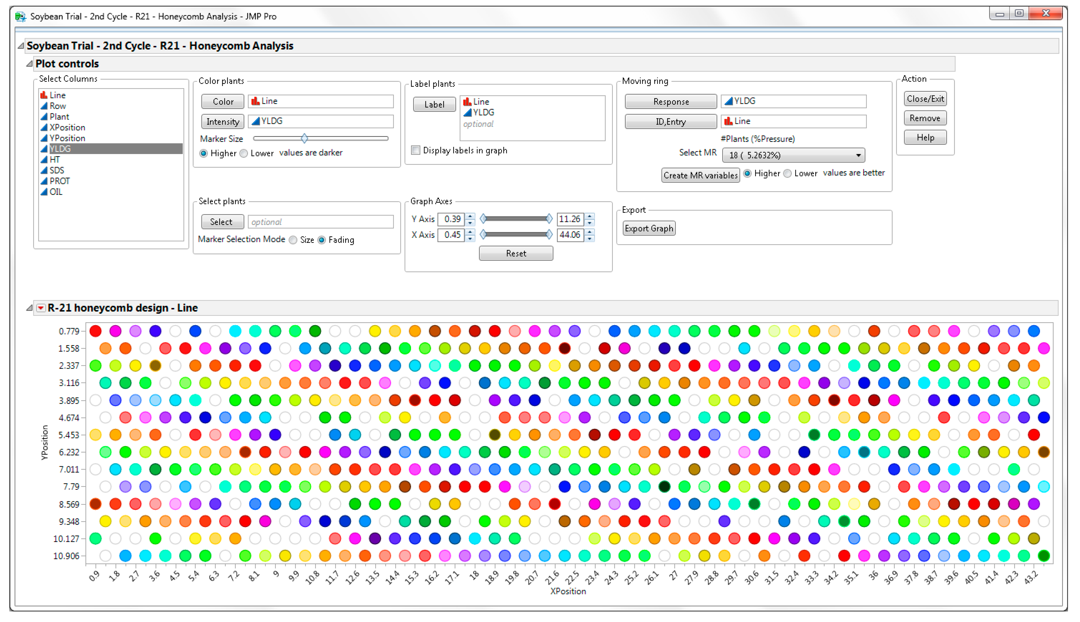
Honeycomb Analysis table script embedded within the JMP table (upper left side). The program generates the graphic view of the design with Plot Controls (Figure 11) that allow the user to visualize data points, analyze the data, and select plants. The user can assign the Line and the trait of interest (YLDG) columns to the Label role. The values of these columns are displayed in a pop-up window when the mouse hovers over the point in the graph.
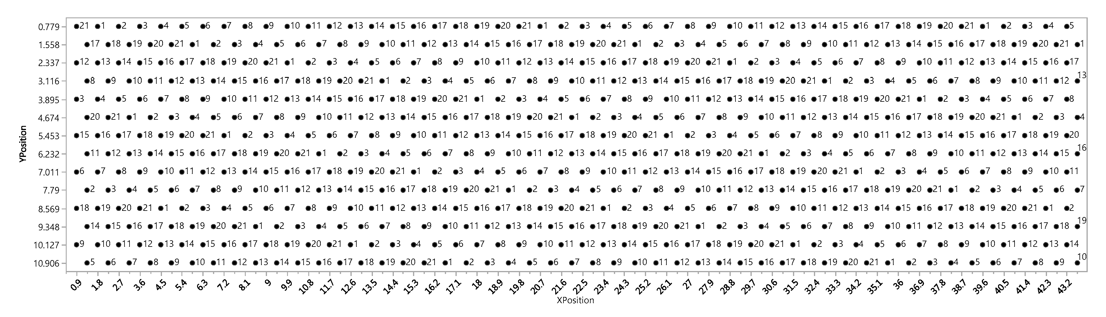
The user can also visualize the R-21 design by labeling plants by Line and displaying labels in the graph (Figure 12).
Assign the trait of interest (YLDG) to the Moving Ring Response role. Verify that the Line column is assigned to the Moving Ring Entry role (Figure 11). Select the Moving Ring size. In this case, we chose a ring size of 18 plants. Then press the 
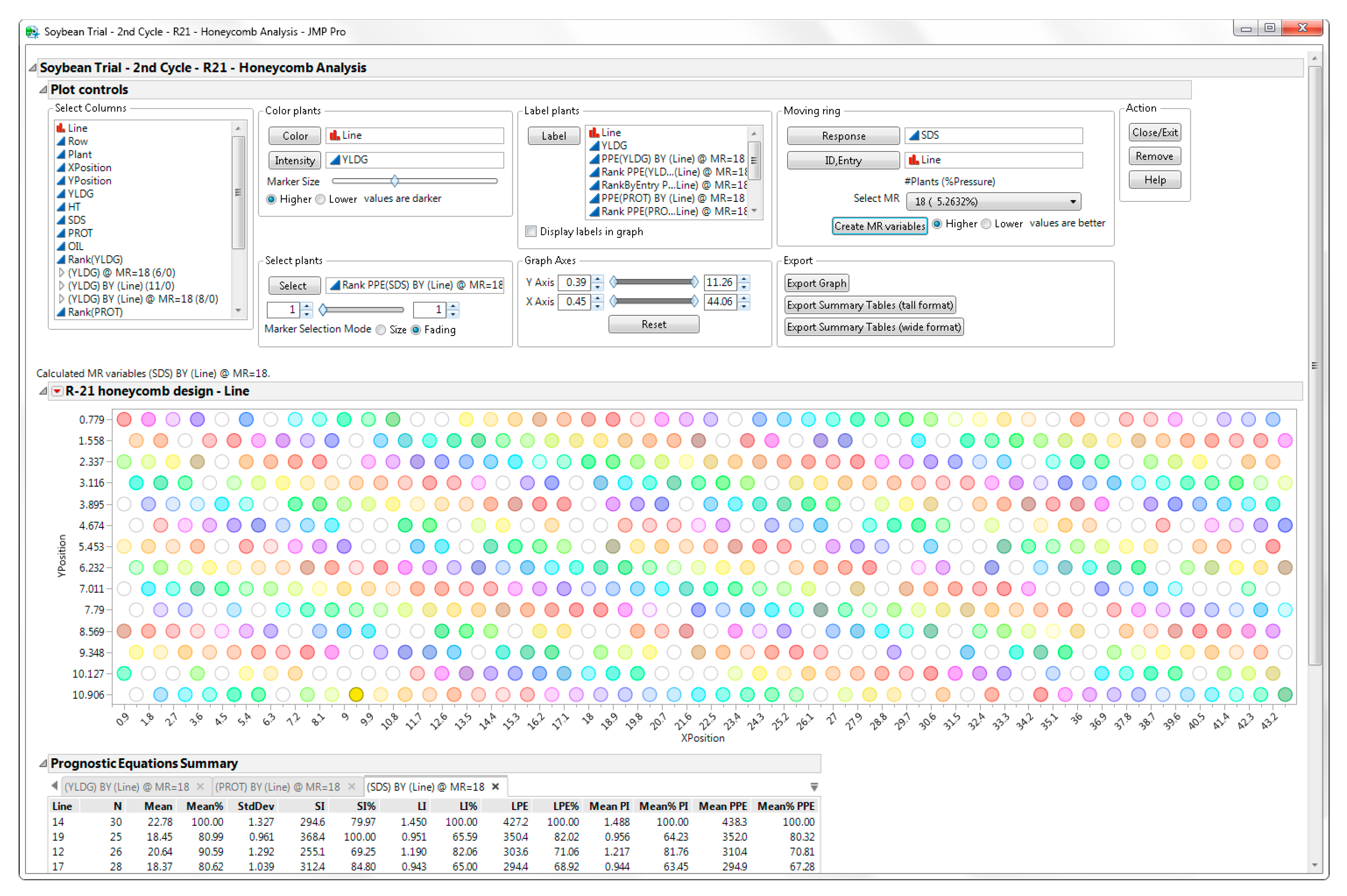
Create MR variables button. Various moving ring variables are added to the JMP table. For replicated designs, the JMP program generates a summary table that includes the Line Prognostic Equation (LPE) and the line average of the Plant Prognostic Equation (MeanPPE) used for selection of the best lines.
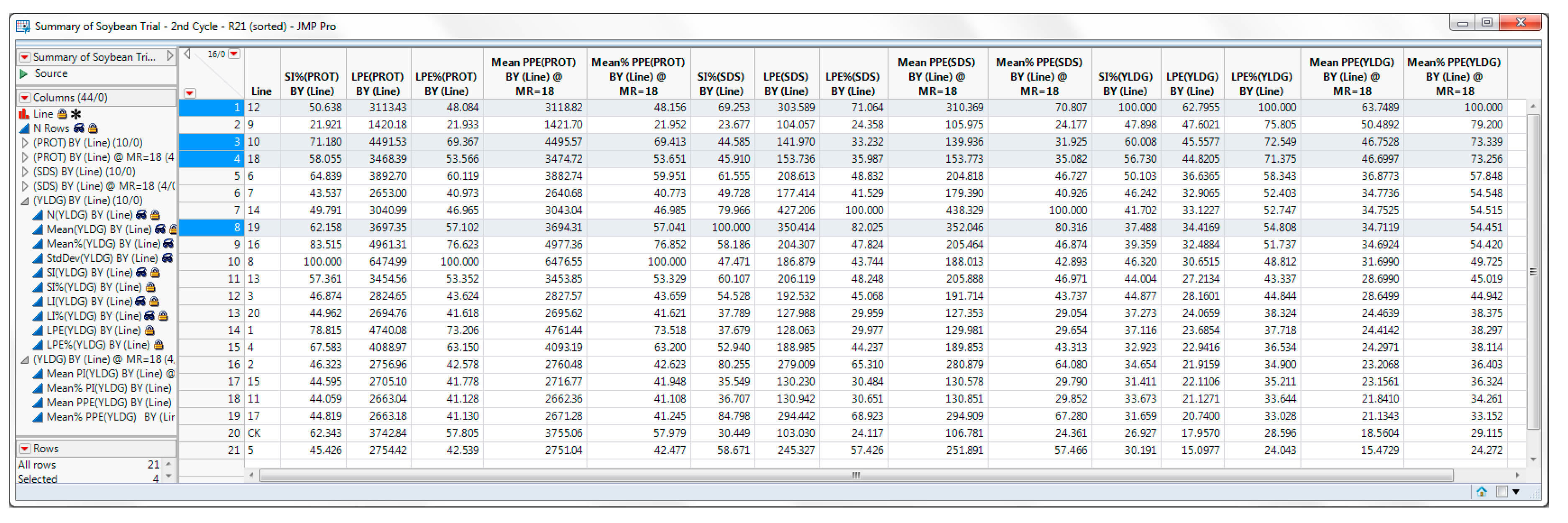
Summary Table calculates N (no. plants/line), Mean and Std Deviation of the trait, SI, LI, LPE, MeanPI, MeanPPE. To more easily compare lines and get the resolution range, selected variables are rescaled with respect to their maximum value (Mean%, SI%, LI%, LPE%, Mean%PI, Mean%PPE) (Figure 13).
Selection of the best lines for YLDG is performed by ranking the lines by their LPE or MeanPPE [2]. The two prognostic equations are similar since they both measure concurrently plant yield potential and stability of performance. Based on MeanPPE, the 4 best lines for YLDG are lines 12, 9, 10 and 18 with MeanPPE values of 63.75, 50.49, 46.75, and 46.70, respectively. Compared to lines 12, 10 and 18, line 9 has the highest plant yield index (MeanPI = 1.49) but it has low Stability Index (SI = 33.76). Since stability is the most important component for Crop Yield, line 9 is dropped from further consideration.
Line 12 has the highest MeanPPE = 63.75 and the best SI = 70.5, meaning that line 12 has high stability of performance. An important point to make is that line 12 has a relatively low yield potential (MeanPI = 0.9) and it would not have been selected if it did not have a very high SI, demonstrating the significance of selecting concurrently for yield potential and stability by using the PPE. The check line (Haskell) is on the bottom of the table with low MeanPPE = 18.56 and a low SI (Figure 13).
Selection based on PPE or LPE magnifies the differences among lines [2]. The resolving power of the MeanPPE, expressed by the resolution range of the Mean%PPE(YLDG) (25–100%), is much larger than the resolving power of Mean%(YLDG) (71–100%) (Figure 13). This suggests that PPE has a better predictive and resolving power, thus selection is much more efficient when using the PPE. The user can visualize these differences by creating a chart using standard JMP tools (Figure 14).
In conclusion, the best 3 lines selected for high crop yield potential (based on PPE) are lines 12, 10 and 18, with line 12 being the most important one. The superiority of line 12 was confirmed when grown in Randomized Complete Block (RCB) trials across 4 years and 17 different environments at commercial plant densities. Across all environments, line 12 exhibited a 5% statistically significant seed yield superiority compared to the check cultivar (CK), demonstrating the importance of selecting concurrently for plant yield and stability [2].
Selection of the best plants within the selected lines is performed by ranking the plants within the selected lines by PPE. You can use a data filter to select lines 12, 10 and 18. Create a subset JMP table of these lines. By sorting the subset table by RankByEntryPPE, you can select the best 6 plants from each of these lines. These 18 plants, along with foundation seed as a check, can be promoted to the next cycle using a Replicated-19 honeycomb design.
Selection of the best lines for multiple traits, (i.e., YLDG, PROT, SDS) can be performed by creating moving ring variables and summary tables for each of the traits. The user assigns each of the additional traits, PROT and SDS, to the Moving Ring Response role and presses the Create MR variables button for each trait (Figure 15). Summary tables for each trait are generated.
One important thing to note is that line 9 has consistently low Stability Index (low SI) across all different traits, YLDG, PROT and SDS, thus, it is excluded from further consideration. SI is a powerful parameter for selecting lines that have good trait stability and low SI values denote unstable lines.
There are different ways to select for multiple traits and every breeder may have different priorities. One way is to rank the lines based upon the prognostic equation (LPE or MeanPPE) for YLDG. Eliminate any lines with a low SI. Further reduce the number of lines in consideration to select only the best ones based upon the values of prognostic equations (LPE or MeanPPE) for the remaining traits: PROT and SDS.
It may be easier to select for multiple traits using a combined summary table. Press the Export Summary Table (wide format) button (shown in Figure 15) to create a combined summary data table (Figure 16). Use standard JMP tools to subset and sort this table to aid in the selection. Since yield is the most important trait, sort the table by LPE%(YLDG) or Mean%PPE(YLDG), descending. The best lines should lie towards the top of the table. To check for stability, reorder the columns, placing the SI% columns at the front of the table. Line 9, although it has the second highest LPE%(YLDG), has a low SI among YLDG, PROT and SDS, thus it is removed from further consideration.
To select the best lines, reorder the columns, placing the LPE% columns for the desired traits at the front of the table. Line 12 appears to be the best line for the trait YLDG. The breeder can use standard JMP tools to calculate a weighted average of the LPE% with weights 3,1,1 for YLDG, PROT, SDS, respectively. This lists the best 5 lines as 12, 10, 14, 18, 19. A weighted average of the LPE% with weights 3,2,1 for YLDG, PROT, SDS, respectively, lists the best 5 lines as 12, 8, 10, 19, 18. It seems reasonable that the best 4 lines for YLDG, PROT, SDS are lines 12, 10, 18, 19. The breeder can then select the best plants within these lines based upon the highest PPE of the most important trait.

4. Conclusions

This technical note presents the development of a powerful JMP Add-In program as a useful tool for the construction of different honeycomb designs and the analysis of data in prognostic breeding methodology for efficient selection of the best entries and the best plants per entry based on the indices and the prognostic equations. Use of the prognostic equations speeds up the early stages of plant selection and accelerates the annual genetic gain. By rapidly computing the selection criteria for plant yield and stability, the program increases efficiency and provides the foundation for potential mechanization.
The Prognostic Breeding Application JMP Add-In program displays powerful controls allowing the user to create maps of any honeycomb design and visualize the selected plants in the field. Standard JMP tools can be employed to subset and sort tables to aid in the selection process across traits, years and locations.

Supplementary Materials

The following are available online at https://www.mdpi.com/2073-4395/9/1/25/s1, Program File S1: Prognostic Breeding Application Ver 6-2018-08-17.JMPAddIn.

Author Contributions

All the authors contributed to the work in the paper. V.A.F. performed the field experiments, computed data, and wrote the manuscript. K.C.T. wrote the JMP Add-In program, computed data, and provided suggestions. A.M. computed data and provided suggestions and project supervision. All authors reviewed the manuscript.

Funding

This research received no external funding.

Conflicts of Interest

The authors declare no conflict of interest.

References

  1. Duvick, D.N.; Smith, J.S.C.; Cooper, M. Long-term selection in a commercial hybrid maize breeding program. In Plant Breeding Reviews; Janick, J., Ed.; John Wiley & Sons: New York, NY, USA, 2004; Volume 24, pp. 109–151. [Google Scholar]
  2. Fasoula, V.A. Prognostic Breeding: A new paradigm for crop improvement. In Plant Breeding Reviews; Janick, J., Ed.; John Wiley & Sons: New York, NY, USA, 2013; Volume 37, pp. 297–347. [Google Scholar]
  3. Fasoula, D.A.; Fasoula, V.A. Competitive ability and plant breeding. In Plant Breeding Reviews; Janick, J., Ed.; John Wiley & Sons: New York, NY, USA, 1997; Volume 14, pp. 89–138. [Google Scholar]
  4. Fasoula, V.A.; Fasoula, D.A. Honeycomb breeding: Principles and applications. In Plant Breeding Reviews; Janick, J., Ed.; John Wiley & Sons: New York, NY, USA, 2000; Volume 18, pp. 177–250. [Google Scholar]
  5. Fasoula, V.A.; Fasoula, D.A. Principles underlying genetic improvement for high and stable crop yield potential. Field Crops Res. 2002, 75, 191–209. [Google Scholar] [CrossRef]
  6. Fasoula, V.A.; Tollenaar, M. The impact of plant population density on crop yield and response to selection in maize. Maydica 2005, 50, 39–48. [Google Scholar]
  7. Uphoff, N.; Fasoula, V.A.; Iswandi, A.; Kassam, A.; Thakur, A.K. Improving the phenotypic expression of rice genotypes: Rethinking “intensification” for production systems and selection practices for rice breeding. Crop J. 2015, 3, 174–189. [Google Scholar] [CrossRef] [Green Version]
  8. Fasoulas, A.C.; Fasoula, V.A. Honeycomb selection designs. In Plant Breeding Reviews; Janick, J., Ed.; John Wiley & Sons: New York, NY, USA, 1995; Volume 13, pp. 87–139. [Google Scholar]
  9. Fasoula, D.A.; Fasoula, V.A. Gene action and plant breeding. In Plant Breeding Reviews; Janick, J., Ed.; John Wiley & Sons: New York, NY, USA, 1997; Volume 15, pp. 315–374. [Google Scholar]
  10. Fasoula, V.A. A novel equation paves the way for an everlasting revolution with cultivars characterized by high and stable crop yield and quality. In Proceedings of the 11th National Hellenic Conference in Genetics and Plant Breeding, Orestiada, Greece, 31 October–2 November 2006; pp. 7–14. [Google Scholar]
  11. Fasoula, V.A. Two novel whole-plant field phenotyping equations maximize selection efficiency. In Modern Variety Breeding for Present and Future Needs, Proceedings of the 18th Eucarpia General Congress, Valencia, Spain, 9–12 September 2008; Prohens, J., Badenes, M.L., Eds.; Editorial Universidad Politecnica de Valencia Publisher: Valencia, Spain, 2008; pp. 361–365. [Google Scholar]
  12. Greveniotis, V.; Fasoula, V.A. Application of prognostic breeding in maize. Crop and Pasture Sci. 2016, 67, 605–620. [Google Scholar] [CrossRef]
  13. Mauromoustakos, A.; Fasoula, V.A.; Thompson, K.C. Honeycomb designs computing and analysis. In Proceedings of the International Biometric Society, Eastern North American Region, Tampa, FL, USA, 26–29 March 2006. [Google Scholar]
  14. Mauromoustakos, A.; Thompson, K.C.; Fasoula, V.A. Honeycomb Designs Addin; JMP Discovery Summit: Frankfurt, Germany, 2018; Available online: https://community.jmp.com/t5/Discovery-Summit-Europe-2018/Honeycomb-Designs-Add-In-new-version/ta-p/52961 (accessed on 9 March 2018).
  15. Rasmusson, D.C.; Phillips, R.L. Plant breeding progress and genetic diversity from de novo variation and elevated epistasis. Crop Sci. 1997, 37, 303–310. [Google Scholar] [CrossRef]
  16. Peterson, P.A. The plant genetics discovery of the century: Transposable elements in maize. Early beginning to 1990. Maydica 2005, 50, 321–338. [Google Scholar]
  17. Haun, W.J.; Hyten, D.L.; Xu, W.W.; Gerhardt, D.J.; Albert, T.J.; Richmond, T.; Jeddeloh, J.A.; Jia, G.; Springer, N.M.; Vance, C.P.; et al. The composition and origins of genomic variation among individuals of the soybean reference cultivar Williams 82. Plant Physiol. 2011, 155, 645–655. [Google Scholar] [CrossRef] [PubMed]
  18. Cullis, C.A. DNA rearrangements in response to environmental stress. Adv. Genet. 1990, 28, 73–97. [Google Scholar]
  19. Brunner, S.; Tingley, S.; Rafalski, A.; Fengler, K.; Morgante, M. Evolution of DNA sequence nonhomologies among maize inbreds. Plant Cell 2005, 17, 343–360. [Google Scholar] [CrossRef] [PubMed]
  20. Dudley, J.W.; Lambert, R.J. 100 generations of selection for oil and protein in corn. In Plant Breeding Reviews; Janick, J., Ed.; John Wiley & Sons: New York, NY, USA, 2004; Volume 24, pp. 79–110. [Google Scholar]
  21. Moose, S.P.; Dudley, J.W.; Rocheford, T.R. Maize selection passes the century mark: A unique resource for 21st century genomics. Trends Plant Sci. 2004, 9, 358–364. [Google Scholar] [CrossRef] [PubMed]
Figure 1. A partial list of replicated honeycomb designs, obtained when the X and Y take values from 0 to 9. The bold numbers in the center of the squares are the allowable number R of entries. The numbers in the corners are the K parameters, used for the identification of the starting number of each row. The X, Y and K are internal parameters necessary for the construction of the designs [8]. Formation of moving replicates/rings and moving triangular grids applies to all the honeycomb designs.
Agronomy 09 00025 g001
Figure 2. The Replicated-21 honeycomb design evaluates plants of 21 lines (entries). Each plant is placed in the center of a moving replicate/ring (green circles), allowing the use of the plant yield index (PI) for measuring plant yield devoid of the confounding effects of soil heterogeneity [2]. Plants of each line are placed in the corners of a moving triangular grid (shown here for line no. 9) which ensures effective sampling for soil heterogeneity and allows effective measurement of the stability index (SI).
Agronomy 09 00025 g002
Figure 3. Construction of the UN (unreplicated) honeycomb design with 30 rows and 14 plants per row.
Agronomy 09 00025 g003
Figure 4. JMP data table generated according to the specified Unreplicated honeycomb design. Entry, Row, Plant, XPosition and YPosition columns are displayed.
Agronomy 09 00025 g004
Figure 5. Graphic view of the unreplicated honeycomb design stored in the JMP table. The graph shows the layout of the plants according to the honeycomb design, while the intensity of the blue provides a quick visual of the lowest and highest-yielding plants.
Agronomy 09 00025 g005
Figure 6. Graphic view of the best 21 plants in the unreplicated honeycomb design, selected based on high plant yield index PI(YLD).
Agronomy 09 00025 g006
Figure 7. JMP table showing the best 20 plants selected (one border plant was dropped) for the next cycle based on PI(YLD).
Agronomy 09 00025 g007
Figure 8. Soybean plants grown in the R-21 honeycomb design with a plant spacing of 0.9 m.
Agronomy 09 00025 g008
Figure 9. Construction of the R-21 honeycomb design with 14 rows and 48 plants per row.
Agronomy 09 00025 g009
Figure 10. JMP Table generated according to the specified R-21 honeycomb design with data collected for seed yield, height, seed size, seed protein and seed oil.
Agronomy 09 00025 g010
Figure 11. Graphic view of the R-21 honeycomb design stored in the JMP table. The graph shows the layout of the plants according to the specified design (14 rows and 48 plants/row). The 21 lines have been labeled by different colors and shaded by the intensity of YLDG (using the Color and Intensity button). White circles represent missing plants.
Agronomy 09 00025 g011
Figure 12. Graphic display of the R-21 honeycomb design, showing the layout of the 21 lines in 14 rows and 48 plants per row.
Agronomy 09 00025 g012
Figure 13. Summary table of the R-21 honeycomb design that computes the indices and the prognostic equations used for the selection of best lines.
Agronomy 09 00025 g013
Figure 14. Chart of the Mean%(YLDG) and Mean%PPE(YLDG) of the 21 lines using the Tabulate option in JMP. Resolution range is larger in the Mean%PPE and selection becomes more effective.
Agronomy 09 00025 g014
Figure 15. Plot controls, graphic view of the R-21 honeycomb design, and Prognostic Equations summary table generated by the JMP program for the selection of best lines for YLDG, PROT, SDS.
Agronomy 09 00025 g015
Figure 16. Combined summary JMP table for YLDG, PROT and SDS generated by using the Export Summary Table (wide format) option in the JMP program.
Agronomy 09 00025 g016

