An Assessment of Low-Cost Techniques to Measure Ammonia Emission from Multi-Plots: A Case Study with Urea Fertilization

Abstract

Ammonia (NH₃) emission from agriculture is an environmental threat and a loss of nitrogen for crop production. Mineral fertilizers and manure are significant sources of NH₃; therefore, abatement technologies have been introduced to mitigate these emissions. The aim of this study was to demonstrate that low-cost measuring techniques are suitable to assess NH₃ emissions in smaller plots, appropriate to test different managements. Two experiments were established to quantify NH₃ emissions from urea application in a multi-plot design with radii of 5 (R5) and 20 m (R20). Field was bare soil partially surrounded by shelterbelts. Measurement techniques included passive flux samplers (Leuning), and passive concentration samplers (ALPHA) coupled to WindTrax dispersion model. NH₃ emission from R5 was consistent with the emission from R20 when the surface-to-atmosphere exchange was not affected by shelterbelts, and wind speed near surface was greater than 1 m s⁻¹. Both measurement methods gave unreliable NH₃ quantification in combination with wind speed lower than 1 m s⁻¹ and low emission strength. Cumulative emission over 60 h was 2% of the supplied N from the plots not affected by the shelterbelt, and 1% from the plots affected by shelterbelts, indicating that these structures can significantly reduce NH₃ emissions.

1. Introduction

Emission of ammonia (NH₃) from the application of mineral fertilizers and animal manure to agricultural surfaces represents a consistent loss of reactive nitrogen [1] which farmers must compensate with additional nitrogen. The emitted NH₃ represents a serious threat to human health, because it reacts with sulfuric, nitric, and hydrochloric acids in the atmosphere [2] forming fine particles (PM_2.5) that cause lung diseases [3,4]. Furthermore, once emitted from the source and dispersed in the atmosphere, half of the NH₃ is dry deposited in form of gas to natural ecosystems within few kilometers, while the other part is transformed to ammonium aerosols and contribute to wet deposition over long distances (from 100 to 1000 of kilometers) [5]. These depositions contributing directly to exceed the critical nitrogen loads of the ecosystems, causing eutrophication [6,7,8]. Agriculture is the main source of NH₃ in the atmosphere [1,9], therefore this sector must reduce emissions (United Nations Economic Commission for Europe, UNECE, Convention on Long-range Transboundary Air Pollution [10]), and the European Union has established that NH₃ emission from the Member States must be reduced below the limits set by the National Emission Ceilings Directive [11].

Efficient application technologies able to reduce the N-emissions from manure and mineral fertilizer spread on the field are needed to comply with the European directives. Concurrently, valid and suitable measurement methods are necessary to evaluate the performances of these technologies and support their development [12]. In the last decades, most of the tests performed on NH₃ volatilization from manure and mineral fertilizers at field-scale or in in agronomic plots, were measured with the Integrated Horizontal Flux (IHF) technique, the ZINST method, the inverse dispersion modelling (IDM) coupled with concentration measurements, or with wind tunnels [13,14,15]. Agronomic plots of 20 m in radius treated with manure are the most common design in the tests of low emitting spreading technologies [14], and the IHF is often considered as a reference method to assess NH₃ emissions [12,16]. In the typical tests, IHF is used to measure emission from relatively large plots (radius of 20 m) which demands a large distance between coexisting plots to avoid advection interferences; consequently, few or no replications at plot-level are carried out. This can be avoided by reducing the commonly used plot size [17], therewith increasing the number of plots established in the same field and assessing multiple products, replicates, or multiple factors that play a role in the mechanisms of ammonia emission.

To date, there is still a need for a method easy to deploy under real field conditions to better characterize the dynamics of NH₃ emissions as affected by agronomic practices. Unfortunately, there are no low-cost NH₃ analyzers to deploy in multiple-plots experiments. This is due to the technical difficulties of measuring highly reactive gases as NH₃, as well as to the costs of the equipment. Low-cost instrumentation, as passive diffusion sensors, could provide a solution since they offer the possibility to be widespread and to measure emissions from more plots at the same time.

Alongside the emission abatement techniques related to the application of the fertilizers in the field, existing structures in the edges of the agricultural surfaces such as hedgerows (e.g., windshield barriers, flood regulation, enhance biodiversity and increase landscape diversity) may also reduce the surface-to-atmosphere exchange limiting NH₃ emissions. However, the literature about the effect of these barriers on ammonia emission is still lacking. Moreover, Danish farmers have traditionally established shelterbelt as a common strategy to shield the fields from the fierce prevailing Atlantic winds.

In this study, we quantified NH₃ emissions from urea application in two experiments in a multiple large- and a small-plot design. Ammonia emission was assessed with two micrometeorological methods, the passive concentration samplers (ALPHA, [18]) coupled to IDM, and the IHF where the flux above the plot was directly measured with passive flux Leuning samplers [19]. The ALPHA samplers were used in three plots of 5 m radius, varying the proximity to a shelterbelt (15 to 33 m gap). A plot of 20 m radius was located 50 m from the shelterbelts and was included for control using ALPHA and passive flux Leuning samplers.

To facilitate selection of the best set-up for NH₃ measurements in circular plots we calculated the unique height H_ZINST for measuring NH₃ horizontal flux. This height represents the point where the ratio of horizontal to vertical fluxes are relatively unaffected by atmospheric stability [20], giving the most precise results when calculating the vertical flux with the IDM or the ZINST model. The ZINST transfer factor K_ZINST and the H_ZINST are given for circular plots with a range of diameters and surface roughness (Z₀).

2. Material and Methods

Treatments: The study was carried out in September 2017 at Aarhus University’s experimental research station in Aarslev, Funen, Denmark (55°18′44.9″ N, 10°26′18.6″ E). The soil is classified as a sandy loam, Typic Agrudalf, with 1.1% C, 70% sand, 15% silt and 13% clay, and a pH_CaCl2 of 6.3 in the 0 to 0.5 m soil layer [21]. The experimental site was covered by winter wheat stubble that had a height of 10 cm above the soil surface, the crop was harvested one week prior to the experiment, resulting in a surface roughness length of Z₀ = 2 cm [22]. A circular plot with a radius of 20 m (R20; “Plot 1”) and three plots with the radius 5 m (R5; “Plot 2” to “Plot 4”) were established on the field to execute ammonia measurements. Furthermore, in the north-east edge of the field there was a 3 m high hedgerow (Figure 1), while in the west side a fence with sparse small trees. The distance from the plots to the nearest hedges on the field border was equal to, or larger than, five times the height of the hedges, which should assure that the measurements calculated using the IDM is reliable [23,24].

Urea (46% N) in prills was applied on 1 September 2017 8:00 a.m. and again on 5 September 08:00 a.m., each time at a rate of 200 kg N ha⁻¹. Through hand-held fertilization, a homogeneous and precise application was achieved by dividing the plots into smaller sectors.

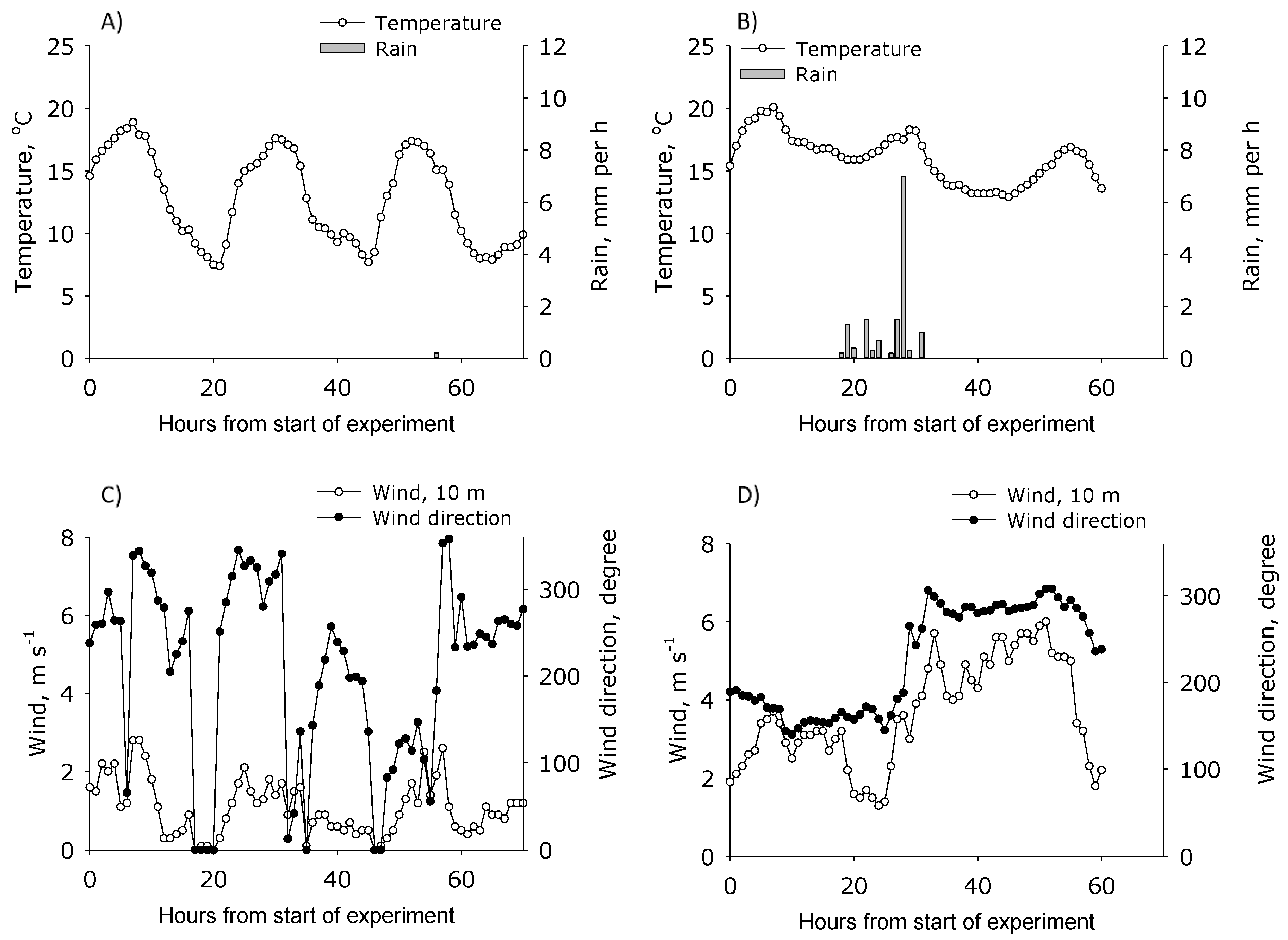
Wind speed (10.0 m height), rain (1.50 m height) and temperature (2.0 m height) were acquired by a nearby (<350 m) weather station and recorded as hourly averages (Figure 2) by the national Danish Meteorological Institute. Moreover, to calculate the emission, wind speed was measured at 5 min average at the H_ZINST heights, 1.0 m for the R20 plot and 0.57 m for the R5 plots, by means of 3-cup anemometers coupled with Wind101A Data Loggers (MadgeTech, Inc., Warner, NH, USA).

Emission fluxes from all plots were estimated using IDM combined with wind speed and NH₃ concentration measurements, while also directly by means of flux samplers in Plot1. In Plot 1 in fact, emission was assessed with the IHF method set-up with the Leuning passive flux samplers placed at heights of 0.6, 1.0, 1.8, and 2.45 m from the soil surface. For the IDM calculation the vertical flux (or the emission) was estimated from wind speed measurements at the H_ZINST heights, and NH₃ concentration measured with four ALPHA samplers [25] placed at the same H_ZINST. The emission was measured from 1 September 2017 8:00 a.m. till 4 September 2017 9:00 a.m., and on 5 September 2017 8:00 a.m. hours till 7 September 2017 9:00 p.m. Measurement intervals were 4 h during daytime and 12 h at night-time.

Background flux was measured using the Leuning passive flux samplers at 1 m height, and NH₃ background concentration was determined in the same position with ALPHA samplers at 0.57 m height.

Leuning flux samplers: the wind weighted average horizontal flux of NH₃ ($\overline{F_{hor}}$, μg NH₃-N m⁻² s⁻¹) was measured with the Leuning passive flux samplers [19]. The horizontal flux was derived from

$$\overline{F_{hor}}=\frac{M}{At}$$

(1)

where M is the mass of NH₃ absorbed (μg NH₃-N) by acid solution in the passive flux sampler during the sampling period t (s), and A is the effective cross-sectional area of the sampler orifice ($A=0.63\times A_1$), where A₁ is the area of the orifice in m². Coating solution for the flux samplers was prepared with oxalic acid dissolved in acetone, according to the procedure outlined in the study of Leuning et al. [19]. After exposure, the coating solution was dissolved in 0.04 L of deionized water and the NH₄⁺-N(aq) content of this solution was determined by an ammonia ion selective electrode (ISE) and a Hach HQ411d pH/mV voltmeter (Hach Company, Loveland, CO, USA).

ALPHA Samplers: Adapted Low-cost Passive High Absorption (ALPHA; [25]) samplers are a system designed for the measurement of the concentration of NH₃ in air. They consist in a polyethylene container that work on the principle of gaseous diffusion through a polytetrafluoroethylene (PTFE) membrane (27 mm radius, 5 μm pore size, 305 μm thickness), where the emitted NH₃ is absorbed to an inner filter paper (24 mm radius grade 604) coated with citric acid (13% m/v). NH₃ measurements were carried out above the emitting sources, in the center of the plots, by means of a set of four passive samplers exposed at the same position. After exposure, absorbed NH₃ was leached using 4 mL deionized water and quantified with the ammonia ion selective electrode [26]. The concentration (μg NH₃-N m⁻³) was related to the absorbed mass of NH₃ (M) by Fick’s Law of diffusion [18]:

$$\overline{N{H}_3}=\frac{M_{sample}-M_{control}}{V}$$

(2)

where V (m³) is the effective volume of sampled air, given by V(t) = 0.0032 × t [18], where time t is given in seconds. During the trials, a set of samplers were placed in the center of each plot to measure the NH₃ concentration (M_sample), while the background, or control concentration (M_control) was assessed by another set of samplers placed west of the experimental plots in the same position of the background flux measured with the Leuning samplers (Figure 1). ALPHA samplers were purchased from Centre for Ecology and Hydrology of the Natural Environment Research Council (Penicuik, Great Britain).

This passive sensor, together with the Leuning flux samplers, offer low-cost alternatives to measure surface-to-atmosphere exchange fluxes, as the cost of the components of the ALPHA to perform one filed trial as presented here is estimated to be of the order of a 3500€. In the same way, the cost of the Leuning samplers are around 8000€. These costs must be added to the chemical analysis of the samples and the determination of the ancillary measurements.

Calculating the ZINST height and K_ZINST value: in the middle of the circular Plot 1, there is a height, H_ZINST, where the horizontal flux ($\overline{F_{hor}}$) divided by the emission (F; g NH₃-N s⁻¹ m⁻²) is constant, regardless of the atmospheric stability [26]. Therefore, a measurement of the horizontal flux, which is equal to the product of wind speed (U; m s⁻¹) and the NH₃ concentration (C; g NH₃-N m⁻³) defines the emission across all meteorological conditions at this height. This simplifies the requirements of field measurement and reduces the need for in depth micrometeorological competences, because there is no need to measure turbulence parameters as friction velocity (u *, m s⁻¹) and defined atmospheric stability (Monin Obukov length, L). Finally, to perform this quantification, only the knowledge of U and C at the ZINST height, and the K_ZINST value $\left(K_{zinst}=U\times C/F\right)$, which is related to plot radius and surface roughness length (Z₀; cm), are needed.

Both H_ZINST and K_ZINST were estimated in silico with a set of simulations using the IDM method by means of the backward Lagrangian Stochastic “bLS” model WindTrax (Thunder Beach Scientific, Halifax, NS, Canada). The IDM model can calculate the concentration at a given location in space and time, knowing the source strength (Q). In the simulations performed the emission of NH₃ was set arbitrarily to 0.5 kg NH₃-N ha⁻¹ h⁻¹ (as both H_ZINST and K_ZINST should be independent of the emission at this height) and was emitted from circular plots of radius equal to 5, 10, 15, and 20 m. The NH₃ concentrations were calculated at the heights of 0.3, 0.6, 0.7, 0.8, 0.9, 1.0, 1.1, 1.3, 1.5, 1.7 and 2 m using fixed values of L equal to −10 m, +10 m, and infinitely large; wind speed was calculated for the same heights, except for the height of 1 m, which was set to 1 m s⁻¹. Then the ratio $U\times C/Q=K_{zinst}$ was plotted versus the heights and H_ZINST was determined as the height where the three K_ZINST profiles of different L matched. The value is obtained with an approximation, as there may not be an exact matching height value for all three profiles. If no exact match was reached then the height with lowest difference between $U\times C/Q$ profiles was chosen, or if the variation was larger than 5% no K_ZINST was provided. The obtained height is the H_ZINST at which the horizontal flux must be measured for the given radius and Z₀. K_ZINST is the parameter for this plot size and surface that must be used in the calculations of emissions from the plot using the ZINST approach, i.e., the emission is calculated as follows: $Q=U\times C/K_{zinst}$.

Calculating emission: The IHF technique was used to calculate the NH₃ emission rate from the circular Plot 1, F_IHF (μg NH₃-N m⁻² s⁻¹), by the difference in the horizontal fluxes (F_net(z), μg NH₃-N m⁻² s⁻¹) of gas across down- and upwind boundaries measured at different heights (Equations (3)–(5)). It has been shown that the relationship between the logarithm of height and F_net(z) is linear (Equation (4)) and that the vertical flux of ammonia can be calculated with Equations (3)–(5) [27]:

$$F_{net}(z)=F_{hor,dw}-F_{hor,uw}$$

(3)

$$F_{net}(z)=a\ln (z)+b$$

(4)

$$F_{IHF}=\frac{1}{X}{[ah\ln (z)-az+bz]}_{z_0}^{z_p}$$

(5)

where dw and uw denotes the horizontal flux down- and upwind the plot, and X (m) is the distance travelled by the wind across the plot. The integration limit z_p is the height at which the F_net is at background level.

The IDM (Equation (6)) was used to calculate the emission from all plots using the NH₃ concentration measured by absorption with ALPHA samplers and wind speed with anemometers at the H_ZINST. The model infers the emission (F_IDM) from the plots knowing the time-averaged concentration of NH₃, ($\overline{C}$, μg NH₃-N m⁻³), measured at one single height in each plot over the integration period, the mean wind speed ($\overline{U}$, m s⁻¹) together with wind direction (WD, °N), a fixed and estimated value of the roughness length (z_o, m) and the value of the Monin-Obukhov length L [28].

$$F_{IDM}=\frac{\overline{C}}{{\left(\frac{C}{F}\right)}_{sim}}$$

(6)

In Equation (6), the WindTrax model was applied to calculate the time-averaged trace concentration to flux ratio (C/F)_sim at the same location of the concentration measurements in the field, within the plume. This parameter is obtained from the number of intersections and the velocity of thousands of upwind trajectories released from the location where the concentration was measured for each time step, that hit the emitting surface (“touchdowns”). The time-averaged concentration $\overline{C}$ is the difference between the measured NH₃ concentration and the background.

Finally, the ZINST technique assesses the emission (F_ZINST) from the measurement of increases in the F_net in the wind passing through the experimental plot at H_ZINST (m) [29]:

$$F_{ZINST}=\frac{\overline{U\times C}}{K_{ZINST}}$$

(7)

3. Results and Discussion

The air temperature during the study ranged between 7 and 20 °C (Figure 2). No rain events occurred during period 1 (1 to 4 September 2017), whereas in period 2 (5 to 7 September 2017) it rained 18–31 h after application of urea with heavy rains of 7 mm h⁻¹ after 28 h. 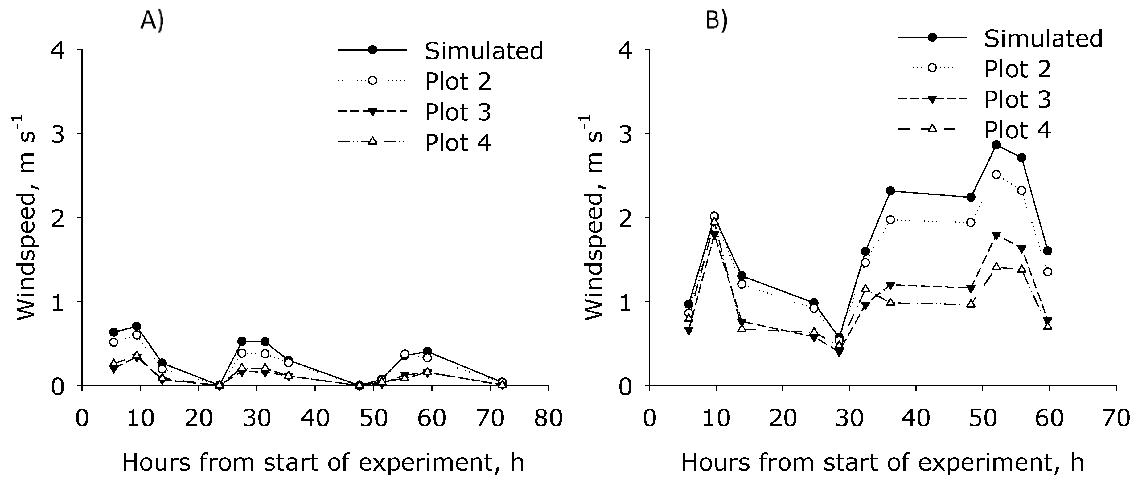In the first experimental period the wind speed measured at 10 m height was between 0 and 3 m s⁻¹, and most of the time lower than 2 m s⁻¹. At all measurements conducted at 0.57 m height, the wind speed was between 0 and 0.8 m s⁻¹ (Figure 3). In the second period, the wind speed at 10 m height ranged between 1 and 6 m s⁻¹ (Figure 2), while at 0.57 m and 1 m height ranged from 0.5 to 3 m s⁻¹ (Figure 3). Using the WindTrax model, the wind speed at 0.57 m height in Plot 2–4, was estimated using the wind speed measured at 10 m height. The simulation indicated that for period 1 and period 2, wind speed in Plot 2 was not affected at 0.57 m height by hedges, while it was reduced with 50% to 75% in Plot 3 and Plot 4 (Figure 3). Additionally, there was found no effect of hedges (providing shelterbelts) in Plot 1. The prevailing wind direction during period 1 was north, east, and south, i.e., most of the time from the edge with a hedgerow, while in period 2 it was north, west, and south, giving less interference from the shelterbelts.

The H_ZINST height for measurement of wind speeds and NH₃ concentrations, and the K_ZINST scaling factor, were estimated for plots of radii 5, 10, 15 and 20 m (

Table 1. The simulated H_ZINST and K_ZINST as a function of different surface characteristics, roughness lengths (Z₀) and plot size. H_ZINST is estimated at Monin Obukov length 10 m, −10 m and 10⁵ m (corresponding to a length of ∞ m) using the IDM model WindTrax. “nr” indicates no result of the assessment or no convergence.

Surface Characteristics	Surface Roughness (Z0, cm) a	Plot Size, Radius (m)
		5		10		15		20
		HZINST (m)	KZINST	HZINST (m)	KZINST	HZINST (m)	KZINST	HZINST (m)	KZINST
Harrowed—no obstacles	0.5 b	nr	nr	nr	nr	0.7	9.1	0.9	9.5
Newly ploughed, Grass (3–5 cm), Wheat stubble (5–10 cm)	2 b	0.5	4.9	0.7	7.0	1.0	7.0	1.1	8.6
Feed lots	3.6 (2–6) a	0.6	4.3	1	4.8	1.3	5.5	1.5	6.4
Wheat 5–10 cm	5 b	1	2.1	1.1	4.5	1.3	5.8	2	4.3
Wheat 0.5–1 m	10 b	nr	nr	nr	nr	nr	nr	nr	nr

^a: Baum et al. [31]; ^b: Guyot [22].

). The K_ZINST calculated using the IDM model (Table 1) was 19% higher than the K_ZINST given by Wilson et al. [26] for a R20 plot and a surface roughness Z₀ = 0.5 cm. This result is similar to the findings of Häni et al. [29], who determined a K_ZINST of about 17–23% higher than the one calculated by Wilson et al. [26]. If atmospheric stability cannot be measured, we recommend using an IDM model to calculate emissions assuming neutral atmospheric stability and horizontal flux data at the H_ZINST height (Table 1) instead of using the K_ZINST factor; this will give the most robust results [30].

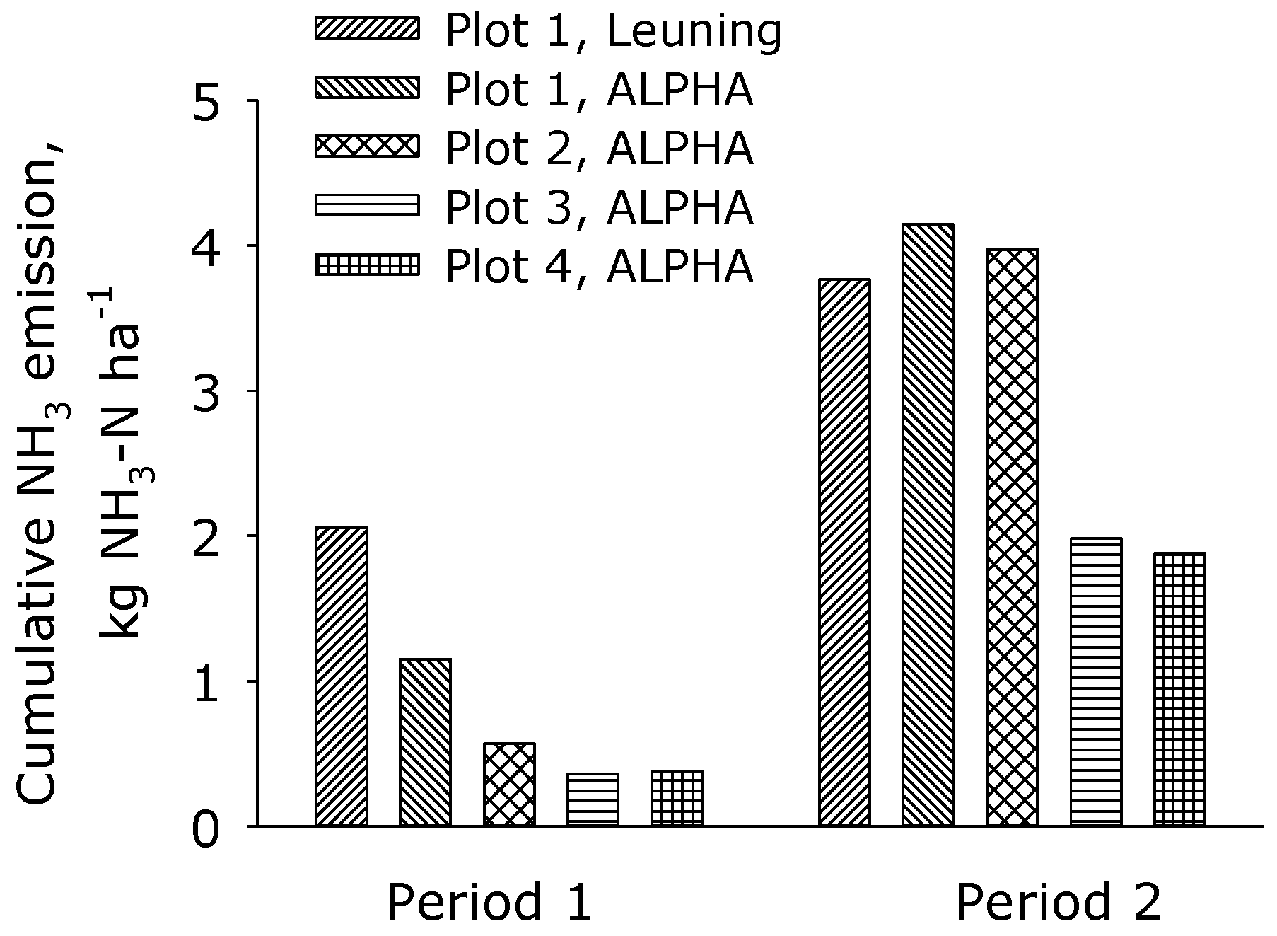
During period 1 the emission from Plot 1 quantified with IHF was higher than those calculated with IDM using ALPHA samplers (Figure 4). This is probably because measurements performed with these techniques are negatively affected by low wind speeds. The Leuning samplers may stall at wind speeds lower than 0.8 m s⁻¹ [19] and it has been shown that the NH₃ captured with passive flux samplers may not be reliable at wind speed lower than 0.92 m s⁻¹ and at low concentrations [32]. At low wind speed and stable atmospheric conditions (night hours), the emission and the transport of NH₃ from surface to atmosphere may be low [33]. Furthermore, at low wind speeds the samplers may be located above the field boundary layer height, especially when a plot size is small [34]. Therefore no, or low, increase in NH₃ concentration is measured at the H_ZINST height during this time. In period 2, wind speed was greater than 1 m s⁻¹ most of the time (Figure 2D) and similar emissions from the R20 plot were measured with the two measuring techniques, IHF coupled with Leuning samplers and IDM coupled with ALPHA samplers.

In period 2 the total cumulative emission from Plot 1 (R20) and Plot 2 (R5) was about 4 kg NH₃-N ha⁻¹ and was also consistent between the measurement techniques within Plot 1. This was expected as wind speed was higher than period 1, or greater than 0.92 m s⁻¹ for the most part of the sampling period. The cumulative emission of Plot 3 and Plot 4 (R5 plots) was almost half of the emission measured on Plot 1 and Plot 2 (2 kg NH₃-N ha⁻¹) (Figure 4). This gap could be explained by the higher wind speed over Plot 1 and Plot 2, which was similar over these plots not affected by shelterbelts, while simulation clearly indicated that wind speed over Plot 3 and Plot 4 was lower due to the shelter from the hedges. Generally, one would expect less significance of shelterbelts at lower wind speeds, and high significance of shelterbelts when wind speed is high (directly affecting the emissions of ammonia). This is also demonstrated by comparing Figure 2D and Figure 3B, which indicate greater differences at wind speed at 0.57 m height between the plots in periods with high wind speeds measured at 10 m height.

In this study, NH₃ emissions were generally low compared with the literature, probably due to low wind speed registered in period 1 and rain within 24 h after urea application in period 2. Moreover, the emission was further lowered due to a reduction of wind speed over Plot 3 and Plot 4 caused by the shelterbelt, as discussed above. Furthermore, the frequency at which ALPHA are substitute in the field is directly connected to the NH₃ absorbed to the filter papers. This is related to low ammonium (NH₄⁺_(aq)) concentrations in the extraction eluate, that can be close to the limit of detection of the ammonia ISE (LOD = 0.4 µM; [35]), potentially producing biases. To obtain reliable emissions it is recommended that exposure period of ALPHA samplers should be longer than 4 h, as used in this study. Our recommendation is to measure NH₃ concentration at integration intervals of 12 h when plots are 5 m radius and wind speed in the range of this study. On the other hand, larger intervals than 12 h exposure should be avoided, because the uncertainty associated with the flux estimation with IDM is high [34]. Loubet et al. [34] highlighted that passive diffusion samplers coupled with IDM underestimate NH₃ emissions of 8 ± 6% in a typical western European climate with a single source and high integration time, where larger biases could be produced with low wind speed and low emission strengths.

The uncertainty related to the quantification of NH₃ emissions by means of IDM coupled with ALPHA samplers is associated with the coefficient of variation between the replicates of the concentration measurements for each integration time. Since this coefficient between the ALPHA is, on average, 10% for all the plots and for the two experiments, the uncertainty about the measurement has, finally, the same magnitude [36]. The uncertainty related to the use of IDM with integration time samplers, is slightly biased in function of the measurement conditions: plot size, measurement height and integration time. Following Loubet et al. [34], then at the conditions given in this study this bias is almost negligible.

Through this study was highlighted that the size of the plot is not affecting NH₃ emission if the wind speed over the considered plots is not different in magnitude, which also means that the two surfaces must be not far from each other. This result confirms recent findings, showing no significant differences in emission from plot sizes ranging from 80 to 5000 m², and fetch lengths of 5–22 m [17,33,37]. The conclusion here is that there is no significant “oasis effect”, which has been claimed to affect emission downwind the edge of a large field due to increasing NH₃ concentration in the interphase between surface and air [14,38]. Due to measuring the flux as [NH₃] × U, the measuring techniques may overestimate emission with 1–20% for plots at fetch lengths from 20 to 100 m radius [14,34,39]. The largest deviation is measured if Z₀ is large (10 cm) under unstable atmospheric conditions [26]. The overestimation is reduced when using Leuning passive flux samplers, which measure $\overline{C\times U}$ during the exposure period [39]. This study confirms that at low Z₀ (2 cm) the emissions measured with the passive flux samplers and the concentration samplers are similar (Figure 4).

The cumulated emission measured during 60 h was from 0.2% to 1% of the applied nitrogen in period 1, and from 1% to 2 % in period 2. Low wind speed in period 1, the effect of the shelterbelts, and the rainfall that occurred in the period 2 after the fertilizer application, are the most probable cause of low emission of NH₃. Low emission has been reported in earlier studies i.e., the emission from urea may range from 0.1% to 30% [40,41,42,43,44]. Furthermore, in support to our findings, recent studies highlighted that low wind speed and precipitation can significantly affect the emission of NH₃, especially if these events occur within 3 to 24 h from the fertilizer application to the field, i.e., these rain events may reduce NH₃ emission with 30% to 90% [9]. The emissions from urea prills can last from some hours to a few days, depending mainly on the characteristics of soil and weather. In this study, the duration of the measurement was adequate to evaluate total emission because the accumulated emissions reached a plateau 60–72 h from the application of the fertilizer, indicating the end of the volatilization.

Total cumulated emission from Plot 1 and Plot 2 at 60 h from the spreading was similar, but over time the rate of NH₃ emission from Plot 1 differed from Plot 2 (Figure 5). This variation is probably due to differences in soil conditions e.g., low soil moisture may have affected the activity of hydrolysis. The variation in emission patterns owing to soil and local climate conditions can be accounted for by more replicates of a treatment (plot-level replicates), which will demand a reduced plot size. Emission measurements from multiple small adjacent plots may be affected by source advection phenomena that bias the estimation of the emitting source. This problem has recently been solved by Loubet et al. [34] proposing a new method coupling the measurement with time-averaged concentration samplers as ALPHA with IDM. Furthermore, in the period 2 and for the Plot 1 the measured emission rates were different between the IHF (Leuning) and the IDM coupled with ALPHA samplers. This highlights the fact that while the two methods are equivalent in the quantification of the total amount emitted at the end of the trial, different methods are affected differently mainly by surrounding conditions as weather, including rainfall and wind speed, atmospheric stability, and emission strength [45]. Finally, their capabilities under a variety field conditions still must be evaluated in detail. Within Plot 1 and Plot 2 in fact the cumulative emission at discrete points in time may be slightly different given the different effects of temperature, rain, and wind speed (Figure 2B,D) on measurements by ALPHA and Leuning samplers, even if the total cumulative emission was similar after 60 h.

4. Conclusions

Simple and low-cost emission techniques have been assessed to measure NH₃ emission from urea in a multi-plot agronomic design. The results obtained indicated that the two techniques can provide reliable estimates of NH₃ emission from fertilizer applied in the field. Results highlights that the influence of natural or semi-natural structures such as shelterbelts can reduce the emission. The short-term period (60 h) was adequate to assess the overall emission that was 2% of the applied N in the plots not affected by the shelterbelt, and 1% from plots located under the effect of these structures.

The constraints of these techniques are related to an underestimation of the emission under conditions of wind speed lower than 1 m s⁻¹ (at 1 m height) and low emission rates. These techniques are applicable in a wide range of circumstances, since there is no need for power; however, the samplers should be exposed for period of 12 h when urea emissions are assessed. The size of the plot between large and small (diameter of 20 and 5 m, respectively) does not limit the application of the two techniques, since proven to give consistent results. This offers the opportunity to evaluate NH₃ emission from more plots in the same field. Finally, further tests are needed to increase the knowledge about the behavior of these low-cost technique under specific surrounding conditions, such as different weather and source strength.