Article

The Role of Canadian Agriculture in Meeting Increased Global Protein Demand with Low Carbon Emitting Production

by
James A. Dyer
1,*,† and
Xavier P.C. Vergé
2,†
1
Contract Researcher, 122 Hexam Street, Cambridge, Ontario, N3H 3Z9, Canada
2
Contract Researcher; 2055, Carling avenue, #1016, Ottawa, Ontario, K2A 1G6, Canada
*
Author to whom correspondence should be addressed.
These authors contributed equally to this work.
Agronomy 2015, 5(4), 569-586; https://doi.org/10.3390/agronomy5040569
Submission received: 20 September 2015 / Revised: 18 November 2015 / Accepted: 2 December 2015 / Published: 4 December 2015
(This article belongs to the Special Issue Advanced Agronomy with Impact for Food Security)

Abstract

:
Although the demand on agriculture to produce food could double by 2050, changing diets will expand the global demand for protein even faster. Canadian livestock producers will likely expand in response to this market opportunity. Because of the high greenhouse gas (GHG) emissions from animal protein production, the portion of this protein demand that can be met by pulse crops must be considered. The protein basis for GHG emission intensity was assessed for 2006 using a multi-commodity GHG emissions inventory model. Because arable land is required for other agricultural products, protein production and GHG emissions were also assessed on the basis of the land use. GHG emissions per unit of protein are one or two orders of magnitude higher for protein from livestock, particularly ruminants, than for protein from pulses. The protein production from pulses was moderately higher per unit of land than the protein from livestock. This difference was greater when soybeans were the only pulse in the comparison. Protein from livestock, especially ruminants, resulted in much higher GHG emissions per unit of land than the protein from pulses. A shift towards more protein from pulses could assure a better global protein supply and reduce GHG emissions associated with that supply.

1. Introduction

The global demand for protein is rising rapidly. This is largely due to more disposable income in emerging economies and changing dietary preferences in much of the developed world [1]. Dire predictions have been made about a global food crisis for 2050, with global population exceeding nine billion and the effect of more extreme weather on farm productivity around the globe [2,3,4,5]. Global food security is exacerbated by inequitable distribution between rich and poor countries [6]. Nowhere is this inequality more apparent than in access to protein, where grains are increasingly being fed to meat animals, while the world’s poorest people struggle with chronic hunger and poor nutrition. The need to address climate change is the added imperative that pushes food production into a perfect storm situation [7]. As the global community awakens to the reality that all countries and all sectors must do whatever they can to reduce greenhouse gas (GHG) emissions [8], all agricultural products can expect to be evaluated on the basis of their carbon footprints (CF). Since livestock account for 14.5% of global GHG emissions [9], consuming fewer livestock products could significantly lower these emissions [10,11].
This CF scrutiny will be particularly intense for livestock products, which are estimated to be responsible for 18% of greenhouse gases [12]. Dyer et al. argued and demonstrated that the fairest way to assess the CF of livestock production was by protein-based GHG emission intensity [13]. This paper focusses specifically on protein production from both plant and animal sources in Canada as a distinct challenge from food security. It determines how much plant sources can help Canada produce more protein with lower GHG emissions. This paper will quantify the CF of these products and describe three indicators suited to this task. The diversity of protein sources and differences in livestock types and production systems among the Canadian provinces result in significant differences among the CF of protein from those provinces. Therefore, a second goal was to determine how these spatial differences affect the protein CF distribution across the Canadian provinces.

2. Background

Protein is a macronutrient necessary for the proper growth and function of the human body [14]. Although there is some debate over the amount of protein a person needs, a deficiency in protein leads to muscle atrophy and impaired functioning of the human body. Whitbread [14] recommended that the current daily intake for protein should be 46 grams for women aged 19–70 and 56 grams for men aged 19–70. Using food balance sheet data from the Statistics Division from the Food and Agriculture Organization of the United Nations, the ChartsBin Statistics Collector Team [15] defined world daily intake per capita of protein as 77 g, ranging from 100 g in the developed world to as low as 55 g/day in the developing world.
While small grain cereals (particularly hard red wheat) produce proteins, this type of protein is considered to be incomplete, because it lacks some of the amino acids that are found in animal proteins and which are essential to the human diet [16,17]. Legumes (or pulses), however, produce complete proteins. Therefore, plant and animal agriculture can be compared on the basis of their respective supply of “complete” protein. Beans and other legumes are a critical source of protein in many parts of the world [14,18]. They are an inexpensive food, high in fiber, calcium and iron.
Trends and patterns in GHG emissions from livestock and field crops in Canada are often discussed simply on an east-west basis, because agriculture west of the Great Lakes is dominated by the Prairie Provinces, while east of Lake Superior, it is the north shore of Lakes Erie and Ontario and the Saint Lawrence River basin that are the dominant farming regions. To discuss regional differences, the provinces were grouped so that the Atlantic Provinces (AP) (treated as one province), Quebec (QC) and Ontario (ON) were defined as Eastern Canada, and Manitoba (MN), Saskatchewan (SA), Alberta (AB) and British Columbia (BC) were defined as Western Canada. Given the size of Canada and the additional small, but distinct, farming regions in the coastal provinces, these trends and patterns also need to be assessed on a sub-provincial basis, as well as a provincial level. However, reporting results on a sub-provincial scale was beyond the scope of this paper.

3. Materials and Methods

3.1. Selecting the Performance Indicators

The assessment described in this paper is an extension of the previous assessment by Dyer et al. [10], which compared the five major livestock industries on the basis of GHG emissions per unit of protein, but excluded any plant source protein. Furthermore, the animal protein-based GHG emission intensity indicator has been applied to the Canadian sheep industry [19]. This paper will describe the first application of this indicator to compare regions on the basis of total protein supply. The second goal of this paper integrated the plant and animal sources of protein production in each province to show the distribution of protein types across the Canadian provinces. Thus, the assessment described below was applied to all means of producing protein in each province.
Ensuring global food security, especially under anticipated climate change impacts on farmland, will also require that a minimum of land capable of growing food-quality carbohydrates is diverted to protein production. Therefore, the indicators used in this assessment should track GHG emission intensity on the basis of both protein production and land use, as well as protein production on the basis of land use. Thus, these indicators include the land use basis for GHG emission intensity (Indicator 1) and all protein production (Indicator 2), as well as the protein-based intensity for GHG emissions (Indicator 3). The dimensions of these three indicators are the GHG emissions and protein production per ha and the GHG emissions per unit of protein production. To quantify these indicators, an automated computer modelling system was assembled capable of integrating the diversity of factors that define the CF of livestock and pulse crop production.

3.2. Performance Modelling Methodology

The Unified Livestock Industry and Crop Emissions Estimation System (ULICEES), which is a spreadsheet-based inventory model, was used in the assessment of livestock GHG emissions. Since ULICEES has been described in detail elsewhere [20], only the main concepts used in inter-commodity assessment are described in this paper. ULICEES was created by assembling the five groups of livestock-specific GHG computations from the Canadian beef, dairy, pork, poultry and sheep (lamb) industries [19,21,22,23,24] in one spreadsheet file. As well as the direct emissions from livestock, these calculations account for GHG emissions from producing the crops that feed each livestock population and the storage practices and characteristics of manure from each livestock type. ULICEES integrated N2O and fossil CO2 emissions with CH4 emissions from livestock. ULICEES was initially applied to 2001 [20], the most recent year with livestock diet survey data [25]. ULICEES was updated to 2006 [19], the latest year with a complete set of input census data. In order to quantify the indirect, as well as the direct GHG emissions from livestock, the concept of the livestock crop complex (LCC), the land that supports feed production in the livestock industry, was a critical component of ULICEES [20]. ULICEES used the Intergovernmental Panel on Climate Change (IPCC) Tier 2 methodology for enteric methane and the Tier 1 methodology modified for Canadian conditions for N2O emissions [26,27].
For the assessment of GHG emissions from just plant protein, the farm fieldwork fossil fuel energy and emissions (F4E2) model [28] was applied to pulse crops. Since pulses are nitrogen-fixing crops and are assumed to not require N-fertilizer, there should be negligible N2O emissions [27]. Although a range of legumes are cultivated in Canada, only annual legumes, or pulses, are considered in this assessment. The F4E2 output files were also integrated with ULICEES to determine the fossil CO2 emissions associated with livestock production [20]. The F4E2 model was based on farm machinery management coefficients from the American Society of Agricultural Engineers (ASAE) [23] and farm machinery management equations [29,30]. The database generated by the 1996 Farm Energy Use Survey (FEUS) [31] was used to verify the F4E2 model and to calibrate several non-fieldwork terms in the farm energy budget.
The pulse crops that were destined for animal feed had to be excluded from the comparison of proteins from pulses to avoid double counting those pulses that are already counted indirectly for their contribution to animal protein production. Since those pulse crops were used for animal feed, they would, therefore, contribute to the protein production by livestock. The livestock diet data used in ULICEES identified these crops as soybeans and dry peas [20]. To correct for this potential double counting of protein production, the areas in those pulse crops that were designated by ULICEES as being in the LCC were subtracted from the crop area statistics. Because ULICEES identifies LCC areas by diet requirements and yields, rather than empirically, more land was identified in these two crops in some provinces than was in the crop statistics. In these cases, the areas that would produce food-quality pulses were assumed to be zero. Whereas this does not guarantee that the soybeans and dry peas outside the LCC were not eventually consumed by livestock, they were at least sold on the market and into another province or the USA.
There were several limitations of this assessment. First, it did not credit ruminant livestock production with any sequestration of soil carbon. That was because this assessment was limited to one year and did not consider any land use transfers among the protein sources over time. Although ULICEES can accommodate this carbon sink term, it only does so for land in the LCC that has been shifted into or out of perennial ground cover (forage) [20]. The second limitation of this study was that it did not take into account the processing energy of any of the agricultural products considered in this paper. A full life cycle assessment of each of the commodities considered in this assessment, such as done for the Canadian dairy industry [32], would have been too involved to include in this paper. This assessment also excluded the potential non-CF risks associated with livestock in Canada [33]. The energy budget for pulses also did not consider the potential of vegetable oils. Soy oil, for example, is one of the feedstocks for biodiesel production [34] and is a popular cooking oil [35].
The processing of soy into tofu can raise the CF of the soybean crop by a factor of four, due to the need to remove most of the oil and ferment the soy meal [36]. However, soybeans are consumed in their whole food form (cooked whole beans versus soy protein alone) throughout Asia [37]. Therefore, besides giving soybeans a higher market value (which was beyond the scope of this paper), converting them into soymilk or tofu is not essential to the consumption of soybeans throughout the world. Therefore, including tofu production in the CF of soybean protein from a theoretical perspective is unnecessary in the context of this paper.

3.3. Defining Protein Conversion Factors

Table 1 provides the protein conversions that were used in this paper for both plant and animal protein sources. Except for lamb, all of the protein conversion factors (PCF) from live weight (LW) were taken from Dyer et al. [13]. The PCF for lamb was taken from Dyer et al. [19]. The PCF for sheep was lower than those for the other three meat animals. Two of these factors had to be expressed as weight of protein per head because the primary products from those animals, milk and eggs, are not their carcasses. The USDA [38] provided the protein contents of one dozen medium-sized eggs as 0.53 kg and of fluid milk as 3.2% by weight [13,21]. For the annual milk yield, the national average for 2006 of 7405 kg/head [21] was used, while the annual egg yield was 186 per layer [21]. The protein from culled dairy cows and unwanted calves was attributed to the beef industry [19], because the slaughtered dairy cows cannot be tracked in the census statistics.
Table 1. Protein conversion factors for five plant (legume) sources and five livestock type sources. LW, live weight. head, one individual producing animal. DM, dry matter.
Plant ProteinAnimal Protein
Pulse Crops% of DM YieldLivestock% of LWKg(protein)/head
Dry peas7.7Beef8.3
Soybeans35.0Dairy237
Lentils9.0Sheep6.4
Chick peas8.9Pork9.8
White beans9.7Layers1.03
Coloured beans8.9Broilers10.1
On the pulse side, PCFs were expressed as the percent of dry matter yield. Using the methodology described by the USDA [38] and nutrition tables published on the USDA website [12,14,34], PCF values were derived for each of the pulses. The highest PCF was for soybeans, which is three- to four-times the PCF of the other pulse PCF (Table 1). This gives soybeans a particularly important role in potential alternate protein sources. The other five pulses have PCFs that are reasonably close to each other. Based on this difference in protein content, the following protein production assessment was applied separately to soybeans and the other pulses.

3.4. Defining the Area Inputs for Protein Production

The design of the assessment process described in this paper depended largely on how land use was distributed among the agricultural products being considered. Figure 1, Figure 2 and Figure 3 summarize the land use inputs to ULICEES and F4E2 that drove the calculations in the three indicators.
Figure 1. Areas (ha × 103) in the pulses (annual legume crops) that were not used to support livestock production in Eastern and Western Canada in 2006.
Agronomy 05 00569 g001
Figure 2. Areas (ha×103) in annual crops (including grains, oilseeds and pulses) used to support different types of livestock in Eastern and Western Canada in 2006.
Agronomy 05 00569 g002
In Figure 1, the general east-west differences among pulse production in Canada indicated which of those crops warranted the closest attention in this assessment. Six pulses were grown on a reportable scale in Canada in 2006, including dry peas, soybeans, lentils, chickpeas, white beans and coloured beans. Soybeans are the predominant pulse crop in the east. No lentils or chickpeas are grown on a reportable scale in the east. In the west, pulse production is more diversified among the six pulses, although areas in dry peas were twice as much as were in lentils, the next highest area.
Figure 3. Areas in annual crops (ha × 103) in each province of Canada used to grow or support three generalized groups of protein sources in 2006.
Agronomy 05 00569 g003
Figure 2 gives an east-west breakdown of the annual crop areas used to produce livestock protein, similar to Figure 1 for pulse protein. Figure 2 implies that the ruminant livestock industries are smaller than they really are because the land in perennial forage was not included in the comparison of land use. This was because this assessment only considered the land base that could be used to produce any of the plant or animal proteins. Consequently, it was assumed that none of the land that was growing perennial forage in 2006 could be used to grow pulse crops. This masks the full magnitude of dairy in relation to pork and the two poultry products as a land user, particularly in Eastern Canada. Nevertheless, the dominant role of western beef and, more importantly, the amount of land capable of growing annual field crops are still apparent.
Figure 3 shows the provincial distributions of all of the land in annual crops that supported protein production in Canada in 2006, including the areas that support ruminants, non-ruminants and pulses. The pulse areas were designated as non-livestock feed use (non-LS) crops because (as explained above) those pulses that support livestock were excluded. Because the areas in pulses are small relative to the crop areas that support livestock in Canada, the soybean areas and areas in non-soybean pulses were recombined into one land use category in Figure 4. The areas attributed to ruminant protein production suggest that the resource use by this livestock system is lower than is really the case because of this exclusion of land in perennial forage.

4. Results

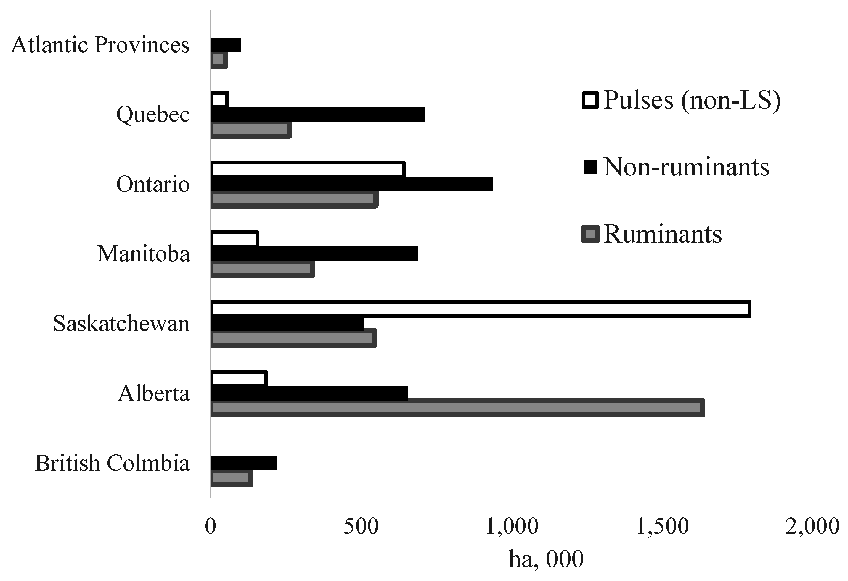
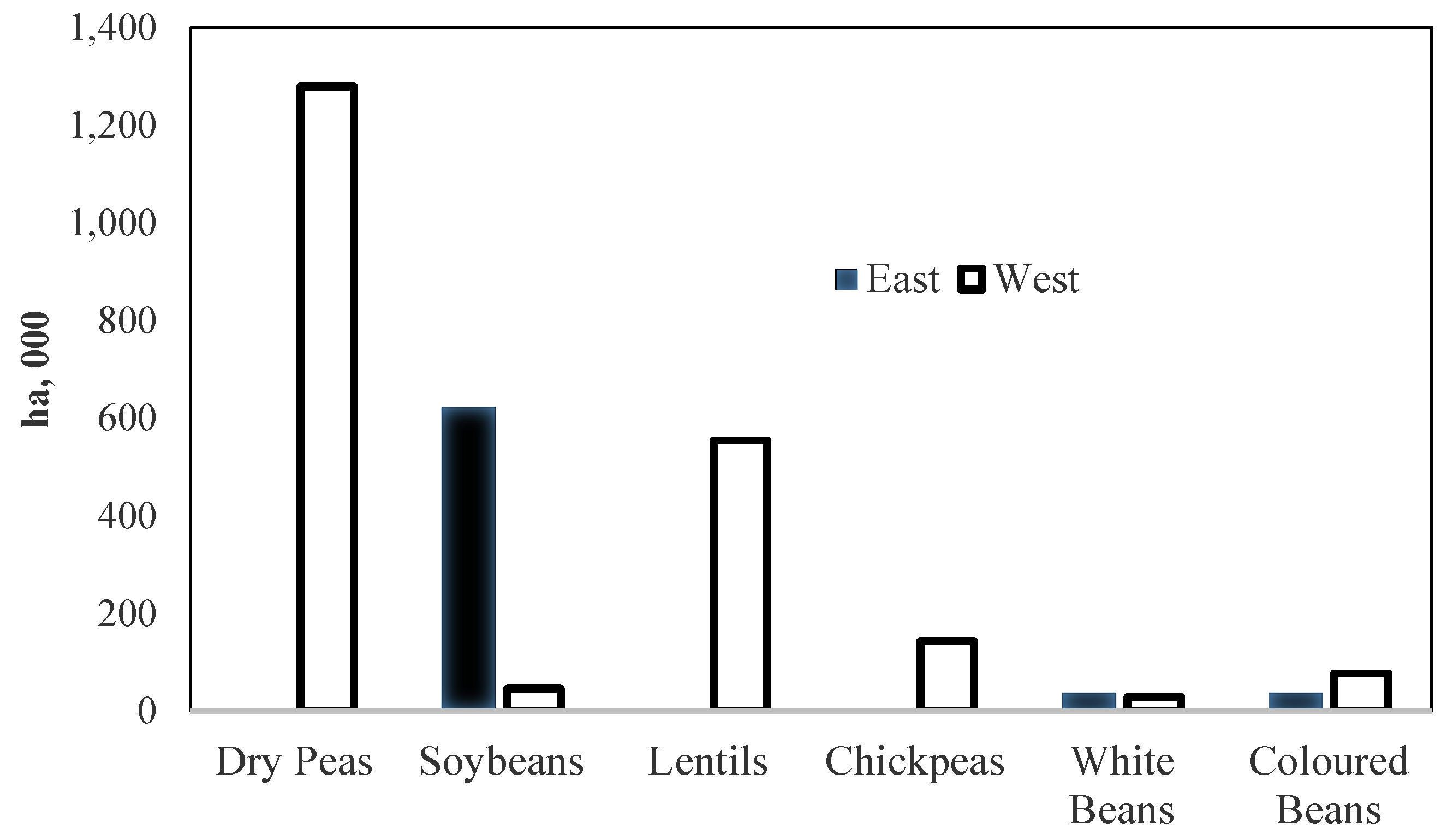
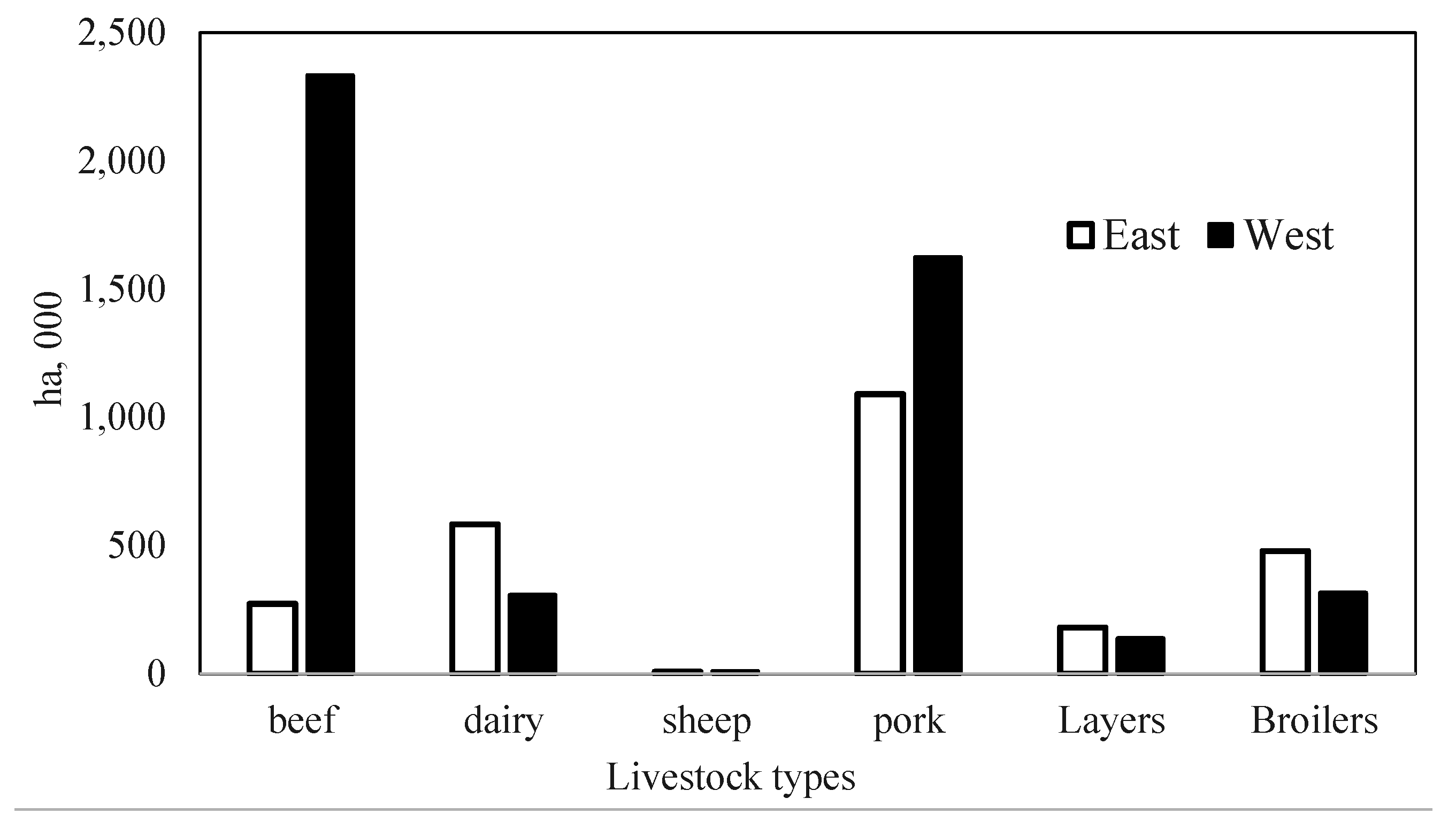
4.1. Area Inputs for Livestock and Pulse Protein Production

In Figure 3, the areas in non-LS pulses were only comparable in size to the areas that support the Canadian livestock industry in Ontario and Saskatchewan. This was mainly due to the dominance of soybeans in Ontario and dry peas in Saskatchewan. Alberta was notable for having much more annual crop land devoted to ruminant livestock due to the large beef population and number of beef feedlots operating in that province [19]. The annual crop land devoted to non-ruminant livestock was relatively evenly distributed across all provinces, although it was the five provinces other than Saskatchewan and Alberta where non-ruminants account for the largest shares of the land that supports protein production.

4.2. Livestock GHG Emissions and Protein Production

Given the importance of enteric methane to the livestock CF [12], livestock commodities were grouped in Table 2 according to whether they were ruminants (which emit copious amounts of enteric methane) and non-ruminants (from which enteric methane is minimal). Table 2 gives a generalized summary of GHG emissions from the Canadian livestock industry for Eastern and Western Canada during 2006. Thus, Table 2 shows the emission estimates from ULICEES [20] for each livestock group and region for CH4, N2O and fossil CO2. Table 2 also shows the estimates from ULICEES for the protein produced by all livestock grouped as ruminants and non-ruminants and on an east-west basis.
Table 2. Total greenhouse emissions (GHG), grouped as being from either ruminant or non-ruminant livestock, and disaggregated by GHG type (CH4, N2O and fossil CO2), as well as protein production (t × 103) from livestock farms in Eastern and Western Canada during 2006.
CH4N2OFossil CO2All GHGProtein
Tg CO2eqt,000
Eastern Canada
Ruminants 17.574.041.4613.07226
Non-ruminants 22.102.211.005.31292
All livestock9.676.252.4618.38518
Western Canada
Ruminants 119.418.502.1430.06274
Non-ruminants 22.051.140.844.03204
All livestock21.479.642.9834.09478
Canada
Ruminants 126.9812.543.6043.12500
Non-ruminants 24.163.351.849.34496
All livestock31.1415.895.4452.46996
1 Includes beef, dairy and sheep (lamb); 2 includes pork, layers (eggs) and broilers.
The two largest sources of GHG in Table 2 were the two methane terms from ruminants, which accounted for 58% of all GHG emissions in the Eastern Canadian ruminants and 65% of the western ruminants. Methane accounted for 40% and 51% of GHG from the non-ruminants in Eastern and Western Canada, respectively. Nitrous oxide emissions accounted for 31% and 28% of all GHG emissions from ruminants in Eastern and Western Canada, respectively, and 42% and 28% of all GHG emissions in Eastern and Western Canada, respectively, from non-ruminants. Fossil CO2 emissions accounted for 11% and 7% from ruminants in the east and west and 19% and 21% from non-ruminants in the east and west, respectively.

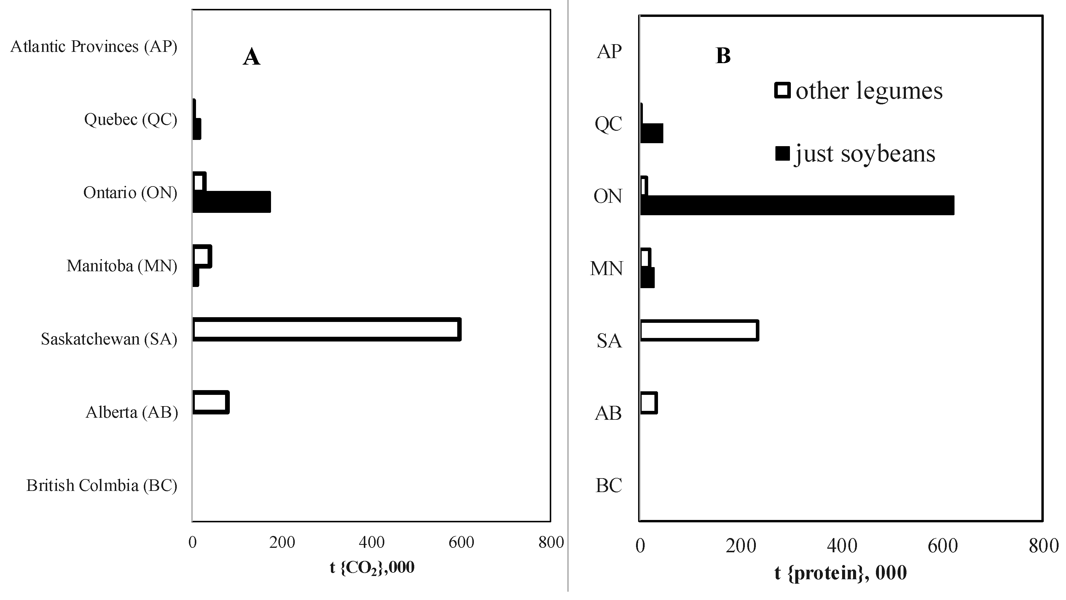
4.3. Pulse GHG Emissions and Protein Production

Figure 4 shows the distribution of pulses across the provinces and illustrates the significance of treating soybeans separately. The GHG emissions and protein production from soybeans was quite distinct from the other pulses among the provinces in 2006. Ontario and Saskatchewan were the only two provinces with significant pulse protein production. Almost all of the soybeans were grown in Ontario, while no reportable soybeans were grown in Saskatchewan. The 2006 Ontario soybean crop emitted a third as much CO2eq as did the Saskatchewan pulse crops, but provided almost three-times as much protein.
Figure 4. Fossil CO2 emissions (A) and protein production (B) from pulses (annual legume crops) grown in each province of Canada in 2006.
Agronomy 05 00569 g004

4.4. Results of Three Indicators for Pulse and Protein Production

Table 3 summarizes the three performance indicators used in this paper for both plant and animal protein production in Eastern and Western Canada in 2006. The combined plant-animal protein production intensities (both pulse and livestock sources) are shown in Table 4 on a provincial basis for 2006. It should be noted that the direction of values considered beneficial for both Table 3 and Table 4 is from low to high in Indicator 2 and from high to low in Indicators 1 and 3. Therefore, in Indicator 2, high numbers mean good, rather than poor, performance.
Table 3 shows that soybeans produced four- to eight-times as much protein per ha as either livestock group in 2006, whereas the area-based protein production of the other pulses was roughly the same order of magnitude as both livestock groups. Excluding soybeans, pulses and the two eastern livestock production systems have similar land use intensities for proteins (Column 3). The land use intensities of non-soy pulses exceeded both of the western livestock production systems (Column 4). For the other two performance indicators, plant protein production showed a dramatic advantage over animal protein (Columns 1, 2, 5 and 6). This was particularly true for soybeans, where ruminant protein emitted 40–50-times as much CO2eq per ha as did soy protein. For the other pulses compared to ruminant animal protein, this emission rates ratio was roughly 35 to one. Even for the other pulses compared to non-ruminant animal protein, the animal protein production had five- to eight-times as high a CO2eq emission rate per ha as did plant protein production. These animal to plant ratios were even more dramatic for CO2eq emission rates per unit of protein, with the ratio of ruminant to soy protein being roughly two orders of magnitude.
Table 3. Greenhouse gas and land use indicators for protein production in Eastern and Western Canada in 2006.
Protein Sources:tCO2/haKg (protein)/hatCO2/t (protein)
Animal:EastWestEastWestEastWest
Ruminants15.1711.3326310357.77109.83
Non-ruminants3.131.821678318.7921.97
Plant:EastWestEastWestEastWest
Soybeans0.300.2610776300.280.42
Other legumes0.410.342071391.982.46
Table 4. Assessment of the integrated protein production on a provincial basis for 2006 in Canada using the three indicators described in this paper, including, the land use basis 1 for GHG emission intensity and all protein 2 production and the protein-based intensity for GHG emissions.
Provinces 3APQCONMNSAABBC
Reporting units
Land 3 use intensity of GHG emissionsIndicator 1
tCO2eq/ha9.37.84.45.23.46.713.0
Land use intensity of protein productionIndicator 2
T (protein)/ha0.230.270.420.150.120.090.32
Protein-based intensity for GHG emissionsIndicator 3
tCO2eq/t (protein)40.428.610.535.227.977.640.3
1 For just land growing annual crops in the livestock crop complex (LCC) and growing non-LS pulses; 2 includes only complete, or animal equivalent, protein; 3 provinces defined using the abbreviations given in Figure 4. Atlantic Provinces: AP; Quebec: QC; Ontario: ON; Manitoba: MN; Saskatchewan: SA; Alberta: AB; British Columbia: BC.
To assess the results from Table 4, provincial rankings over the three indicators were determined. For Indicator 1, the low-to-high rankings were SA, ON, MN, AB, QC, Atlantic Provinces (AP) and, finally, BC. For Indicator 2, the high-to-low rankings were ON, BC, QC, AP, MN, SA and then AB. For Indicator 3, the low-to-high rankings were ON, SA, QC, MN, BC, AP and then AB. Ontario ranked second in Indicator 1 and first in Indicators 2 and 3, giving this province the best overall ranking among provinces. Alberta ranked fourth, seventh and seventh over the three indicators, respectively, making it the overall worst performing province. With rankings of sixth, fourth and sixth over the three indicators, the Atlantic Provinces were the second worst performers overall. Quebec and Manitoba were quite consistently mid-range performers over the three indicators, with rankings of third, fifth and fourth for Manitoba and fifth, third and third for Quebec. The rankings were somewhat inconsistent for Saskatchewan and British Columbia, with rankings of first, sixth and second for Saskatchewan, and seventh, second and fifth for British Columbia over the three indicators.

5. Discussion

5.1. Evaluating Indicator Performance

Although Table 2 showed that ruminants emit far more CH4 than non-ruminants, especially considering that the greatest LW mass of livestock is in beef cattle, the differences between ruminants and non-ruminants were not as much as would be expected from just considering enteric methane. This was because the stored manure from the non-ruminants typically emitted larger quantities of CH4 than did the stored manure from the ruminants (largely due to more liquid manure storage by non-ruminant producers). The east-west differences in N2O emissions between the ruminants and non-ruminants also indicate more liquid manure storage in non-ruminant operations, since dry manure storage typically emits more N2O than liquid manure storage. For livestock, and particularly for ruminants in Western Canada, fossil CO2 emissions were the lowest of the three GHG emissions.
It can be seen in the first two columns of Table 3 (or Indicator 1) that the CF of proteins from pulses was very small compared to the CF of livestock protein. Table 2 partly demonstrates why this would be so. For ruminants, fossil CO2 (the only GHG emitted by pulse production) is around 10% or less of the whole GHG emissions budget of ruminant livestock and 20% of the non-ruminant livestock GHG emissions budget. In addition, the fossil CO2 component of the livestock GHG emissions budget includes the manufacturing of nitrogen fertilizer [20], which accounts for roughly 40% of the fossil CO2 emissions of the fossil energy and CO2 budget of field crops in the LCC. In contrast, fertilizer supply was not included in (and does not contribute to) the CO2 emissions budget for producing the pulse protein. Without including the fertilizer supply term in the livestock CF, the fossil CO2 per ha cost of growing feed grains would be reasonably close to the fossil CO2 per ha cost of growing pulses. In Table 3, pulses also showed a higher rate of protein production per ha (Indicator 2). However, much of this advantage was due to the soybean PCF compared to the other pulses.
Some of the discrepancy among the rankings of provinces for the three indicators in Table 4 can be explained by the differences in the two sub-figures in Figure 4. In Figure 4A, soybean production in Ontario is less than half that of the other pulses grown in Saskatchewan, but the protein production from Ontario soybeans was almost three-times as much as the protein from the other pulses in Saskatchewan. This was due to the much higher protein component (PCF) for soybeans compared to the PCF of the dry peas and lentils grown in Saskatchewan (Table 1). Similarly, the ratios of different annual crop areas of ruminants to non-ruminants among provinces in Figure 3 (taking into account the difference in CF for the two livestock groups) and of western beef in Figure 2 also help to explain why there were some discrepancies in the rankings among the three indicators in Table 4.
The ordinal assessment (rankings) of the three indicators in Table 4 points to Ontario being the most effective protein-producing province in 2006. Saskatchewan should be considered the second best protein-producing province, if allowance is made for the slower growing conditions in the semi-arid cool agro-climate of Saskatchewan compared to BC and the eastern provinces. Alberta was the poorest performing province with the lowest ranks in two of the three indicators. Figure 3 showed that two of the three provinces that ranked lower than Alberta in Indicator 1, BC and AP, had no reportable areas in pulses, while Quebec had quite small areas in pulses. Although Alberta had a large beef herd in 2006, a large portion of these cattle were in feedlots with high energy, low roughage diets, which lowered the enteric methane emissions [22].
Some caution is needed in that this assessment did not consider the processing energy to bring the respective protein to an edible condition for humans. None of the protein sources considered here are edible in their raw state. The top market value of soy products, for example, may be partly offset by the extensive preparation needed to convert it to tofu [36,39]. On the other hand, all of the animal products require refrigeration on their way to market and the dinner table. However, the life cycle assessment for the dairy industry by Vergé et al. [30] found that 90% of the GHG emissions happened before the milk left the farm. Caution is also needed in the equivalency between plant and animal proteins, because this interpretation is largely qualitative. While it is possible to quantify the respective percentages of complete proteins from carcasses and pulses, it seems to be beyond the current state of knowledge what fractions of those two respective protein sources consist of the nine essential, or critical, amino acids that make proteins complete.
Another caution is that the results reported in this paper are specific to Canada. As soybean production expands around the world in response to growing markets, such as China, the displacement of beef cattle by soybeans can have a range of impacts depending on the type of land being shifted from the beef industry to pulse production [4,40,41]. For example, tofu production in European studies has a higher CF than tofu produced from North American soybeans, because the soybeans imported to Europe are largely from Brazil and cause deforestation of the Amazon [5,38].

5.2. Implications for Protein Demand

The last step in this assessment was to interpret protein production estimates in human terms. With a million t of protein from livestock (Table 2) and another million t from pulses (Figure 4B) in Canada and using an approximate requirement for daily intake of protein per capita, a rough estimate of the number of protein person years (PPY), or the number of people per year that can be provided with adequate protein, can be calculated. A rough mid-range value of 70 g of complete protein per capita per day was taken from the daily intake values given above. This calculation suggests that the actual 2006 protein production in Canada could have provided in the order of 78 million PPY, with about half coming from pulses and half from livestock.
From this perspective, it is useful to consider how the conversion of all of the annual crop land in the LCC to pulses might have changed protein production and the CF of that protein. If the 2006 annual crops area in the LCC for all of Canada were taken out of livestock production and reseeded to a combined mix of all of the 2006 pulses, then the protein from this conversion, combined with the protein actually produced from non-LS pulses in 2006, would have provided 141 million PPY from Canada. The mix of pulses across Canada in 2006 resulted in 70% of the non-LS pulse protein being from soybeans and 30% from the other four pulses. If that LCC area were reseeded into just the other pulses (no soybeans), then the combined 2006 protein supply from Canada would have been 80 million PPY. If that LCC area were reseeded into just soybeans, the combined total 2006 protein supply from Canada would have been 340 million PPY.
The CF of this hypothetical all-pulse protein supply scenario would be roughly the same intensity as the actual 2006 protein production shown in Table 3, or 0.33 t CO2/ha. There would be an appreciable difference in the two pulse protein sources, since soybeans yield more protein per weight of crop than the other pulses (Table 1). The protein-based GHG emission intensities (Indicator 3) in Table 3 for the other pulses were four- to six-times higher than for soybeans. However, when compared to livestock, Indicator 3 shows that both sources of pulse protein have orders of magnitude lower protein-based CF values than either the ruminant or non-ruminant protein sources. Caution is needed in interpreting the results of the assessment in this generalized manner, given the potential margins of error in the ULICEES-F4E2 modelling system and the wide range of recommendations in the literature regarding quantity and quality of daily protein intake. In spite of these limitations, the degree of differences between the pulse and livestock protein-based CF cannot be discounted.
Should land growing feed grains for beef be converted to non-LS pulses (as in the PPY scenarios), there remains the potential for the cattle being displaced to be converted back to a more perennial forage diet. While that would mean increased enteric methane emissions from these displaced cattle [22], it could also mean increased soil carbon sequestration, if the land growing that perennial forage were taken from land currently growing annual crops [20]. The PPY scenario did not take these indirect impacts into account, because it was assumed that the cattle being displaced by expanded pulse production would be eliminated. Otherwise, new land has to be brought into the PPY scenario, thus making it too speculative to be of any policy value.
Although hay and pasture are a major resource in ruminant production, potential land use changes were not a factor in this assessment until the displacement of feed grain by non-LS pulse was considered in the PPY scenarios. This transfer of land out of feed grains was at the expense of feedlot cattle, a major part of the Canadian beef industry [20,22]. Thus, as the feedlot cattle go to market, they would not be replaced, and the beef industry would shift back towards cattle being sent directly to market after being raised mainly on hay and pasture. Hence, the amount of hay and pasture would remain mostly unchanged while only the areas in feed grains would decline. A coincidental increase in food demand could also make feed grains more costly and the less intensive pasture-grown beef more profitable than feedlot-finished beef. In contrast to Alexander et al. [5], who defined land displacement as the migration of activities to another place, a cattle population shrinkage was assumed, since the new pulse protein would push beef out of part of its market. There remains the possibility that the displaced feedlot cattle could be transferred to other land. However, this secondary land use change would also result in the pulse protein being an additional protein supply, rather than livestock protein being replaced by pulse protein (as required in the final PPY scenario).

6. Conclusions

The conclusions drawn in this paper relied on all three of the indicators described above. Hence, Indicator 3, the protein-based GHG emission intensity, is most effective when used in conjunction with the two land use indicators. The provinces that ranked best under Indicator 3 were those with the largest areas in non-LS pulses, which is consistent with the lower CF of pulse protein than animal protein. The province ranking the lowest, Alberta, depended heavily on beef and had a relatively small area in pulses. The two coastal provinces (AP and BC) were almost as low as Alberta, which was to be expected, since neither had any reportable non-LS pulse areas.
The results of this protein comparison identified soybeans as having the lowest CF and as being the most effective land use for protein production. In spite of far greater areas in pulses in Saskatchewan, the lower PCF of dry peas and lentils allowed Ontario, the leading soybean producer, to be the highest protein-producing province in 2006. However, caution is needed when an analysis points to just one crop as a wonder crop or super food. There are both nutritional and environmental risks from creating a global-scale dependence on just one crop. On the other hand, the benefits of soybeans derived from this assessment did not include the additional value of that crop as a potential source of biodiesel feedstock [34] or a cooking oil [35], a consideration that would have lowered its net CF even further.
Much of the methodology described in this paper could also be applied in other countries with developed agriculture. In Canada, the two provinces with the lowest CF for protein production, Ontario and Saskatchewan, both on an area and protein basis, also had the largest pulse production. This result suggests that developed countries can reduce the CF of their capacities to produce protein by increasing their consumption and export of pulse protein rather than by producing more livestock. Such extrapolation to other countries, however, should be limited to those regions that do not depend heavily on extensive grazing, because cattle raised primarily on grass have a different CF than cattle raised in the more intensive beef operations typical of North America. In many parts of the world, the soil under the grazing land may not be suitable for annual cultivation, and converting such land to annual crops could lead to serious land degradation.
The two issues identified at the start of this paper, global protein supply and a lower CF for protein production, can both be achieved through a shift in land use towards pulses and away from livestock. Although this analysis also suggests that ruminants are less efficient than non-ruminants with respect to Indicator 3, it should be cautioned that only ruminants can convert perennial forage to protein. However, keeping cattle on low roughage diets (as in feedlots) negates much of the ruminant advantage. The three indicators, particularly 2 and 3, address the global challenges of demand for protein in the human diet and minimizing the GHG emissions from protein production. While expressing the protein production in terms of satisfying global nutritional requirements went beyond the assessment of the three indicators discussed in Table 3 and Table 4, this interpretation has potential food policy value. Inside the farm gate, findings, such as described in this paper, should link with the LCA of whole life cycles when more specific protein products are being assessed.
Although this interpretation is not likely to influence the market strategies of the livestock industries, it should help to position Canada’s role in the global protein supply chain. The PPY concept may be a useful index for evaluating this supply chain on a global scale. The low CF of Canadian soybeans relative to soybeans imported from places where deforestation is a big factor in their CF [38] (such as Brazil) should also help to establish this position for Canada. Since this paper was not aimed at marketing of Canadian pulses, tofu and other meat analogues manufactured from pulses could be removed from the CF calculation of pulses and the scope of this assessment. As a protein supplement to food aid, pulse protein enjoys another advantage over livestock protein, because it can be shipped dry, stored without refrigeration and is usually ready to eat right after boiling.
It must be acknowledged that it is relatively easy to find literature and Internet sources that extol the potential environmental and social benefits of replacing livestock protein with pulse protein. It is somewhat surprising, however, just how much the pulse proteins out-performed the livestock protein as rated by all three indicators within the farm gate. However, the true value of this assessment was not in repeating what some might see as the obvious, but in quantifying the process into a repeatable and scalable package. The level of integration in this modelling system brought all of the variables into one quantitative process (inventory model) that could be applied directly, or rebuilt, in many other countries. Although only 2006 was assessed in this paper, having one computational package will facilitate temporal flexibility by allowing the findings for 2006 to be compared to past or future years (when those data become available) or to hypothetical years that reflect policy scenarios.
In undertaking the second goal of this paper, the disaggregation to provinces, the spatial scalability of this methodology was able to highlight the impact of the inter-provisional diversity of protein sources in Canada. The analysis described in this paper could be applied on a sub-provincial scale, such as ecodistricts and census agricultural regions (CAR). Eventually, international treaties encourage all countries to adopt measures that will mitigate GHG emissions in all sectors. Implementation of such measures for Canadian agriculture will require communication with farming communities on sub-provincial scales (either ecodistricts or CARs). Assuming that the provincial scale inputs used in this assessment are available at these finer scales, this assessment could be repeated at those scales.

Author Contributions

James Dyer was responsible for the design of the study, the generation of the pulse performance data, integration of the livestock and pulse protein estimates, the interpretation of results and for the manuscript preparation. Xavier Vergé was responsible for the ULICEES model, generating the estimates for livestock GHG emissions and contributions to writing the paper.

Conflicts of Interest

The authors declare no conflict of interest.

References

  1. Jacob, B. Global Hunger for Protein Fuels Food-Industry Deals. The Wall Street Journal. 11 June 2014. Available online: http://www.wsj.com/articles/global-hunger-for-protein-fuels-food-industry-deals-1402444464 (accessed on 31 August 2015).
  2. Kelly, T. Impending Crisis: Earth to Run Out of Food by 2050. Time. 7 December 2010. Available online: http://newsfeed.time.com/2010/12/07/impending-crisis-earth-to-run-out-of-food-by-2050/ (accessed on 31 August 2015).
  3. Ritter, K. Climate Change Could Push 100 Million into Extreme Poverty By 2030. The Associated Press. Available online: http://www.huffingtonpost.ca/2015/11/09/climate-change-100-million-poverty-world-bank_n_8509444.html (accessed 10 November 2015).
  4. Smith, P.; Haberl, H.; Popp, A.; Erb, K.-H.; Lauk, C.; Harper, R.; Tubiello, F.N.; de Siqueira, P.A.; Jafari, M.; Sohi, S.; et al. How much land-based greenhouse gas mitigation can be achieved without compromising food security and environmental goals? Glob. Chang. Biol. 2013, 19, 2285–2302. [Google Scholar] [CrossRef] [PubMed]
  5. Alexander, P.; Rounsevell, M.D.A.; Dislich, C.; Dodson, J.R.; Engström, K.; Moran, D. Drivers for global agricultural land use change: The nexus of diet, population, yield and bioenergy. Glob. Environ. Chang. 2015, 35, 138–147. [Google Scholar] [CrossRef]
  6. D’Odorico, P.; Carr, J.A.; Laio, F.; Ridolfi, L.; Vandoni, S. Feeding humanity through global food trade. Earth Future 2014, 2, 458–469. [Google Scholar] [CrossRef]
  7. Cheadle, B. Obama’s Climate-Change Talk Stands in Stark Contrast to Canadian Party Leaders. The Canadian Press. 1 September 2015. Available online: http://www.cbc.ca/news/world/obama-s-climate-change-talk-stands-in-stark-contrast-to-canadian-party-leaders-1.3211523 (accessed on 1 September 2015).
  8. Green, Low-Emission and Climate-Resilient Development Strategies (United Nations Development Programme (UNDP)). 2015. Available online: http://www.undp.org/content/undp/en/home/ourwork/environmentandenergy/focus_areas/climate_strategies.html (accessed on 31 August 2015).
  9. Gerber, P.J.; Steinfeld, H.; Henderson, B.; Mottet, A.; Opio, C.; Dijkman, J.; Falcucci, A.; Tempio, G. Tackling Climate Change Through Livestock—A Global Assessment of Emissions and Mitigation Opportunities; Food and Agriculture Organization of the United Nations (FAO): Rome, Italy, 2013; p. 139. [Google Scholar]
  10. Goodland, R. The Overlooked Climate Solution: Joint Action by Governments, Industry, and Consumers. J. Hum. Secur. 2010, 6. Available online: http://search.informit.com.au/documentSummary;dn=332506353716599;res=IELHSS (accessed on 6 November 2015). [Google Scholar] [CrossRef]
  11. Ripple, W.J.; Smith, P.; Haberl, H.; Montzka, S.A.; McAlpine, C.; Boucher, D.H. Ruminants, climate change and climate policy. Nat. Clim. Chang. Opin. Comment 2014, 4, 2–4. [Google Scholar] [CrossRef]
  12. The Role of Livestock in Climate Change. Available online: http://www.fao.org/agriculture/lead/themes0/climate/en/ (accessed on 31 August 2015).
  13. Dyer, J.A.; Vergé, X.P.C.; Desjardins, R.L.; Worth, D.E. The protein-based GHG emission intensity for livestock products in Canada. J. Sustain. Agric. 2010, 34, 618–629. [Google Scholar] [CrossRef]
  14. Whitbread, D. Top 10 Foods Highest in Protein You Can’t Miss. Health Alicious Ness. 2011. Available online: http://www.healthaliciousness.com/articles/foods-highest-in-protein.php (accessed on 21 August 2015).
  15. ChartsBin Statistics Collector Team (CBSCT). Daily Protein Intake Per Capita. Available online: http://chartsbin.com/view/1155 (accessed on 30 August 2015).
  16. Mack, S. How Many Amino Acids Does the Body Require? Living Strong. Last Updated February 2014. Available online: http://www.livestrong.com/article/463106-how-many-amino-acids-does-the-body-require/ (accessed on 30 August 2015).
  17. Understanding Our Bodies: Amino Acids Are Important. Available online: http://nutritionwonderland.com/2009/07/understanding-our-bodies-amino-acids/ (accessed on 30 August 2015).
  18. Whitbread, D. Beans and Legumes with the Most Protein. HealthAliciousNess. 2011. Available online: http://www.healthaliciousness.com/articles/beans-legumes-highest-protein.php#percent-protein (accessed on 21 August 2015).
  19. Dyer, J.A.; Vergé, X.P.C.; Desjardins, R.L.; Worth, D.E. A comparison of the greenhouse gas emissions from the sheep industry with beef production in Canada. Sustain. Agric. Res. 2014, 3, 65–75. [Google Scholar] [CrossRef]
  20. Vergé, X.P.C.; Dyer, J.A.; Worth, D.; Smith, W.N.; Desjardins, R.L.; McConkey, B.G. A greenhouse gas and soil carbon model for estimating the carbon footprint of livestock production in Canada. Animals 2012, 2, 437–454. [Google Scholar] [CrossRef] [PubMed]
  21. Vergé, X.P.C.; Dyer, J.A.; Desjardins, R.L.; Worth, D. Greenhouse gas emissions from the Canadian dairy industry during 2001. Agric. Syst. 2007, 94, 683–693. [Google Scholar] [CrossRef]
  22. Vergé, X.P.C.; Dyer, J.A.; Desjardins, R.L.; Worth, D. Greenhouse gas emissions from the Canadian beef industry. Agric. Syst. 2008, 98, 126–134. [Google Scholar] [CrossRef]
  23. Vergé, X.P.C.; Dyer, J.A.; Desjardins, R.L.; Worth, D. Greenhouse gas emissions from the Canadian pork industry. Livest. Sci. 2009, 121, 92–101. [Google Scholar] [CrossRef]
  24. Vergé, X.P.C.; Dyer, J.A.; Desjardins, R.L.; Worth, D. Long Term trends in greenhouse gas emissions from the Canadian poultry industry. J. Appl. Poult. Res. 2009, 18, 210–222. [Google Scholar] [CrossRef]
  25. McLaughlin, E.M.; Alain, B. Livestock Feed Requirements Study 1999–2001; Catalogue No. 23–501-XIE; Statistics Canada: Ottawa, ON, Canada, 2003. [Google Scholar]
  26. 2006 IPCC Guidelines for National Greenhouse Gas Inventories, Volume 4 Agriculture, Forestry and Other Land Use. Available online: http://www.ipcc-nggip.iges.or.jp/public/2006gl/vol4.html (accessed on 16 September 2015).
  27. Rochette, P.; Worth, D.E.; Lemke, R.L.; McConkey, B.G.; Pennock, D.J.; Wagner-Riddle, C.; Desjardins, R.L. Estimation of N2O emissions from agricultural soils in Canada. I. Development of a country-specific methodology. Can. J. Anim. Sci. 2008, 88, 1–14. [Google Scholar] [CrossRef]
  28. Dyer, J.A.; Desjardins, R.L. Simulated farm fieldwork, energy consumption and related greenhouse gas emissions in Canada. J. Sustain. Agric. 2003, 34, 618–629. [Google Scholar] [CrossRef]
  29. Finner, M.F. Farm Field Machinery, 2nd ed.; American Printing and Publishing Inc. and Agricultural Engineering, University of Wisconsin: Madison, WI, USA, 1973; p. 226. [Google Scholar]
  30. Jacobs, C.O.; Harrell, W.R. Agricultural Power and Machinery, 1st ed.; McGraw Hill Book Co.: NewYork, NY, USA , 1983; p. 472. Available online: https://books.google.ca/books?id=B2YfAQAAMAAJ&q=ISBN+0070322104 (accessed on 16 September 2015).
  31. A Review of the 1996 Farm Energy Use Survey (FEUS). Available online: http://www.usask.ca/agriculture/caedac/pubs/pindex.html (accessed on 16 September 2015).
  32. Vergé, X.P.C.; Maxime, D.; Dyer, J.A.; Desjardins, R.L.; Arcand, Y.; Vanderzaag, A. Carbon footprint of Canadian dairy products: Calculations and issues. J. Dairy Sci. 2013, 96, 6091–6104. [Google Scholar] [CrossRef] [PubMed]
  33. Dyer, J.A.; Vergé, X.P.C.; Desjardins, R.L.; McConkey, B.G. Assessment of the carbon and non-carbon footprint interactions of livestock production in Eastern and Western Canada. Agroecol. Sustain. Food Syst. 2014, 38, 541–572. [Google Scholar] [CrossRef]
  34. Koc, A.B.; Mudhafer, A.; Fereidouni, M. Soybeans Processing for Biodiesel Production. In Soybean—Applications and Technology; Ng, T.-B., Ed.; InTech. Open Access Publisher: Rijeka, Croatia, 2015; pp. 19–37. [Google Scholar]
  35. The George Mateljan Foundation. Is Soybean Oil Considered a Healthy Oil? 2015. Available online: http://www.whfoods.com/genpage.php?tname=dailytip&dbid=187 (accessed on 9 November 2015).
  36. Plate, T. Tofu’s Carbon Footprint. The Vegetarian Environmentalist. 2015. Available online: http://tofuscarbonfootprint.weebly.com/ (accessed on 6 November 2015).
  37. The George Mateljan Foundation. What’s New and Beneficial about Soybeans? 2015. Available online: http://www.whfoods.com/genpage.php?tname=foodspice&dbid=79 (accessed on 5 November 2015).
  38. USDA National Nutrient Database for Standard Reference, Release 26. Available online: http://www.ars.usda.gov/ba/bhnrc/ndl (accessed on 16 September 2015).
  39. Rastogi, N. How Green Is Tofu? You’d be Surprised to Know. The Green Lantern. 2009. Available online: http://www.slate.com/articles/health_and_science/the_green_lantern/2009/10/how_green_is_tofu.html (accessed on 4 November 2015).
  40. Monahan, J. Soybean Fever Transforms Paraguay. BBC. 6 June 2005. Available online: http://news.bbc.co.uk/2/hi/business/4603729.stm (accessed on 4 November 2015).
  41. Steinfeld, H.; Gerber, P.; Wassenaar, T.; Castel, V.; Rosales, M.; de Haan, C. Livestock’s Role in Climate Change and Air Pollution. In Livestock’s Long Shadow. Environmental Issues and Options; Animal Production and Health Division, Food and Agriculture Organization of the United Nations (FAO): Rome, 2006; Chapter 3; pp. 80–123. [Google Scholar]

