Parameter Calibration and Experimentation of a Discrete Element Model for Tomato Stems

Abstract

Tomato pruning robots are limited by the absence of accurate shear simulation models for tomato stems. Conventional homogeneous discrete element models are incapable of characterizing the multi-layer heterogeneous structure of tomato stems, which gives rise to significant simulation deviations. With Zheza No. 8 tomato stems as research objects, this study measured intrinsic and contact parameters through physical tests and constructed a three-layer bonded discrete element model to simulate the epidermis, xylem and pith with particles of different sizes. Bonding parameters were calibrated using a two-level factorial design, steepest ascent test and Box–Behnken design with shear force as the evaluation index. The optimal parameters reduced simulation errors by 75.8% and 43.7% relative to traditional and pre-optimized models, and accurately reproduced the double-peak shear behavior. The model accuracy improves with xylem maturation, providing a dependable simulation method for the optimization of tomato pruning robots.

1. Introduction

In recent years, the tomato industry has been expanding in scale, having emerged as one of the most important leading agricultural commodities worldwide. Despite its significant economic value and extensive cultivation area, the level of automation in tomato production around the world remains relatively low [1]. Among the various stages of tomato cultivation, the labor costs associated with pruning and harvesting alone account for more than 70% of the total production costs [2].

To address the requirements for automatic pruning, considerable research has been conducted globally on tomato pruning robots. For example, the Dutch company Kompano has developed an automated tomato leaf removal machine capable of managing pruning tasks in a greenhouse covering an area of 2 hectares per day. Other studies have utilized image processing and deep learning techniques to develop visual recognition systems for identifying lateral shoots, thereby improving pruning accuracy [3]. Furthermore, flexible end-effectors have been designed to standardize operations and reduce mechanical damage to plants during pruning [4]. Although significant progress has been made in the development of end-effectors for tomato pruning, the interaction mechanism between these end-effectors and tomato stems remains poorly understood. To reduce experimental costs and enable visual analysis of results, numerical simulation techniques [5] are commonly employed to study interactions between materials and mechanical components. However, existing studies often rely on rigid stem models [6], which fail to simulate key mechanical behaviors of tomato stems during pruning, such as tensile and shear responses. Therefore, to accurately simulate these mechanical processes, it is necessary to develop a breakable Discrete Element Model (DEM) of the tomato stem.

Meanwhile, researchers around the world have conducted in-depth studies on the construction of DEMs for plant stems. Yuan measured parameters of spinach roots, analyzed the shovel-cutting process, investigated the working mechanism, optimized the cutting shovel parameters, and ultimately developed a DEM [7]. Similarly, other scholars have adopted comparable approaches to construct DEMs for flax stems [8], forage rape stems [9], wheat straw [10], and flexible corn stalks [11]. However, in these DEM modeling methods for stems, crops are typically treated as isotropic materials and simplified into a single tissue structure, resulting in Engineering Discrete Element Method (EDEM) simulation models composed of bonded particles with uniform properties. When stems exhibit internal multi-layer structures and anisotropic characteristics, the use of uniformly attributed particles in simulations can lead to significant errors.

To address the issue of significant differences in the mechanical properties between the epidermis and pith of bolting rapeseed stems in the clamping section, Xie et al. [12] employed the Hertz-Mindlin with Bonding contact model and utilized two types of particles with distinct material properties to simulate the epidermis and pith, thereby establishing a double-layer bonded DEM for bolting rapeseed stems at the harvesting stage. Similarly, Zou et al. [13] developed separate discrete element models for the bark and core of ramie stems, simulated the decortication process, and identified the optimal configuration for the ramie stem separation device. Compared to single-layer stem modeling approaches, such methods yield higher accuracy and better reflect the differences in mechanical properties of the internal stem structures.

When establishing a discrete element model, the required parameters mainly include intrinsic parameters, contact parameters, and bonding parameters. Intrinsic parameters consist of Poisson’s ratio, shear modulus, and density; contact parameters include the coefficient of restitution, static friction coefficient, and rolling friction coefficient; bonding parameters mainly comprise normal stiffness, tangential stiffness, critical normal stress, critical tangential stress, and bonding radius. While intrinsic and contact parameters can be directly measured [14,15], bonding parameters are difficult to obtain through direct measurement. Although some bonding parameters can be acquired through measurement and calculation, discrete element models are generally simplified representations, making it challenging to maintain complete consistency between the model and reality. Therefore, validation through both simulation and physical testing is essential [16].

This study focuses on tomato stems and addresses their heterogeneous internal mechanical properties by employing the Hertz-Mindlin with Bonding contact model. A three-layer bonded discrete element method model of the tomato stem was developed using three distinct particle sizes for particle filling. The bonding parameters were subsequently calibrated based on the design of experiments methodology. The calibrated model was then utilized to simulate the mechanical behavior of tomato stems during a shear process. Simulation results demonstrated close agreement with actual shear tests, validating the model’s accuracy. It is noteworthy that existing discrete element method models for crop stems predominantly adopt isotropic and homogeneous assumptions, simplifying the stem structure into a bonded particle assembly with uniform material properties. However, tomato stems exhibit pronounced anatomical heterogeneity, characterized by a radially stratified tissue architecture comprising the epidermis, xylem, and pith. Significant inter-layer variations in fiber content, cellular morphology, and moisture content consequently give rise to gradient mechanical heterogeneity. Conventional rigid models or single-layer homogeneous DEMs are inherently inadequate for accurately capturing these inter-layer mechanical disparities. As a result, during the simulation of the tomato stem pruning shear process, such models fail to realistically reproduce crack initiation sites, propagation trajectories, and the ultimate shear response. Therefore, constructing a three-layer bonded discrete element model that explicitly accounts for the heterogeneous structural characteristics of the epidermis–xylem–pith in tomato stems holds substantial theoretical significance and engineering application value for enhancing simulation fidelity and elucidating the underlying tool–stem interaction mechanisms.

2. Materials and Methods

2.1. Measurement of Tomato Stem Physical Properties

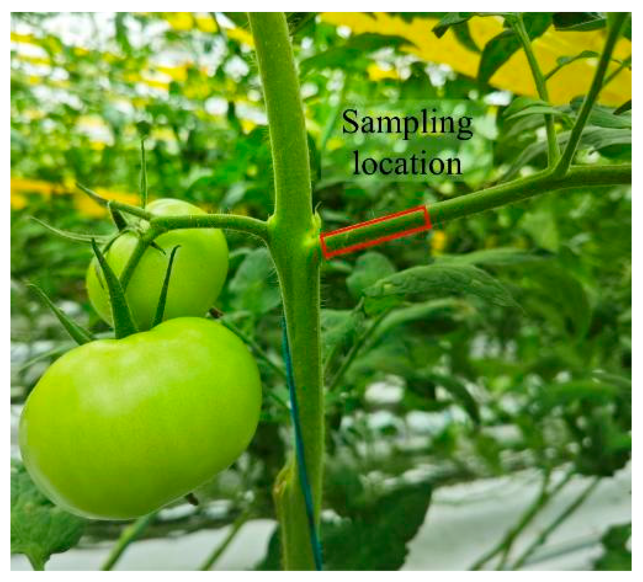
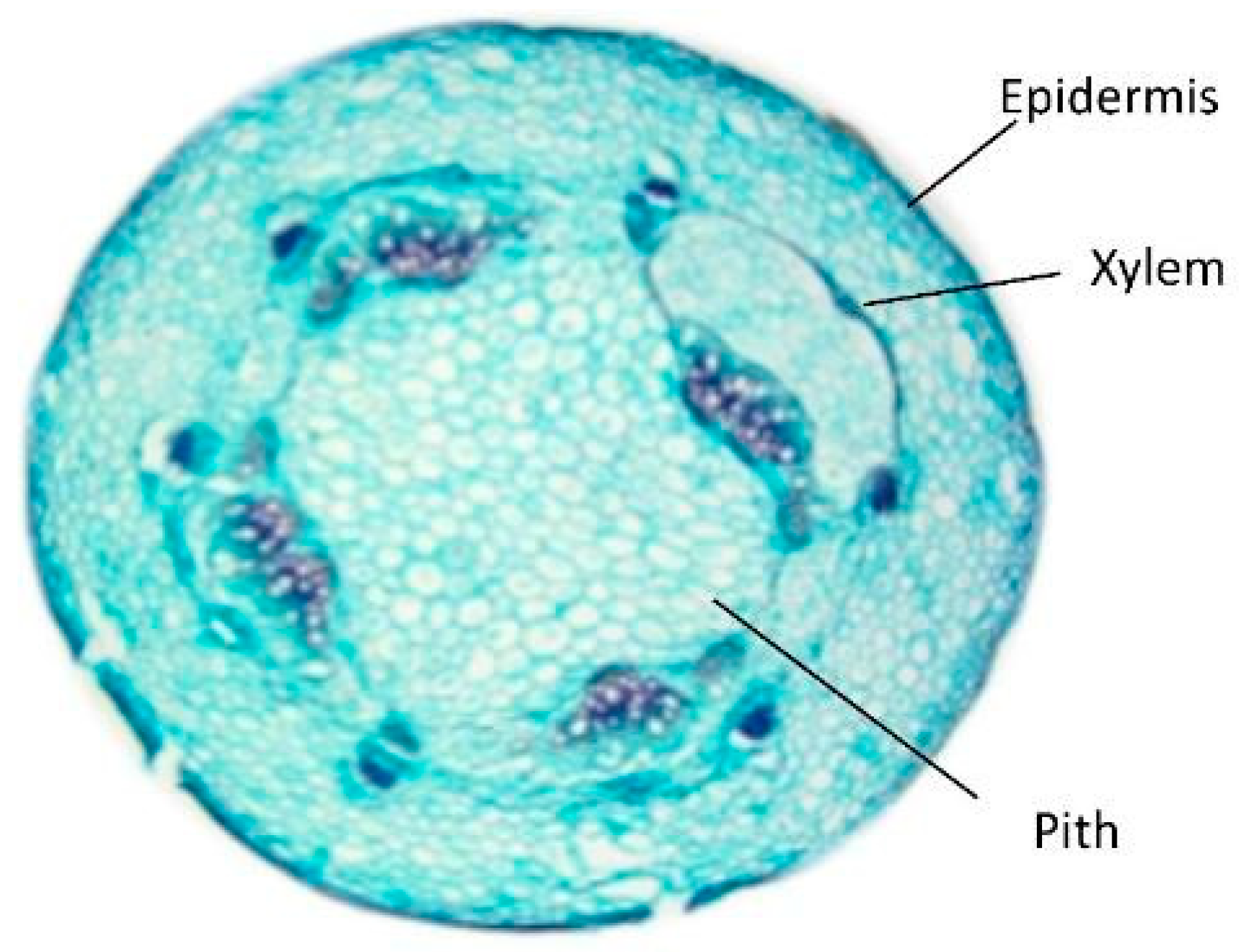
The tomato stems used in the experiment were obtained from the “Zheza No. 8” cultivar of large-fruited tomato grown at the tomato planting base of Shuimu Moganshan Urban Agriculture Complex, Deqing, Huzhou, Zhejiang, China. The study focused on the basal sections of the lateral branches at the early full fruiting stage of the tomato plants, with the specific sampling location illustrated in Figure 1. The internal structure of the tomato stem can be divided into the epidermis, xylem, and pith, as shown in Figure 2. For pruning large tomato plants, the diameter of lateral branches typically ranges from 5 mm to 7.5 mm. Stems with a diameter of approximately 7.5 mm were collected, and their leaves and side shoots were removed. Through repeated measurements and calculations, the following physical property parameters were determined: an average stem length of 50 mm, an average diameter of 7.5 mm, and an average moisture content of 69.5%. To establish an accurate discrete element model for tomato stems and provide reliable physical reference values for the calibration of bonding parameters, this study carried out vertical shear tests on tomato stems using a TMS-PRO texture analyzer produced by FTC (Food Technology Corporation)in Sterling, VA, USA. The instrument was equipped with an S-type load cell with a 500 N capacity and a force measurement accuracy of 0.01 N, and the force signal acquisition frequency was set at 100 Hz. Prior to the test, the instrument was force-calibrated using a 100 N standard weight, with a calibration deviation of ≤0.5%, ensuring that the test accuracy met the experimental requirements. Prior to shearing, the midpoint of the tomato stem was positioned at the cutting groove of the sample platform; once shearing commenced, the force exerted by the cutting tool perpendicular to the cutting groove direction firmly secured the stem on the sample platform, which effectively prevented stem crushing and slippage during the test. Fresh tomato stems were placed horizontally on the fixed platform at the bottom, and a rectangular cutting tool with a thickness of 1 mm and a cutting edge angle of 15° above moved vertically downward along the shearing direction until the stems were completely cut off. To reduce the impact of moisture loss on the mechanical properties of stems, all tests were completed within 2 h after stem picking. The loading speed was set at 2 mm/s, and five repeated tests were conducted on fresh tomato stems with diameters of 3.5 mm, 5.5 mm and 7.5 mm, respectively. The measured average maximum shearing forces were 11.2 N, 17.1 N and 28.9 N correspondingly.

To establish the discrete element model, it was necessary to acquire the intrinsic parameters of tomato stems, including density (ρ), Poisson’s ratio (μ), and shear modulus (G). These parameters were determined through experimental measurements and by referencing existing research findings.

The average density of the tomato stem samples with a diameter of 7.5 mm was determined to be 960.5 kg·m⁻³. To accurately determine the density of tomato stems, given that tomato stems are non-ideal cylinders with irregular cross-sections, the geometric measurement method would induce substantial errors in volume calculation. Accordingly, the water displacement method was employed in this study to measure the volume of tomato stems. Specifically, five tomato stem samples with a diameter of approximately 7.5 mm were selected. Their mass was measured using an electronic balance with a precision of 0.01 g. The samples were then immersed in a round-mouthed beaker filled with distilled water. As the density of tomato stems is slightly lower than that of distilled water, a counterweight with a known volume was used to pull the stems fully submerged. The actual volume of the stems was derived by subtracting the volume of the counterweight from the volume of displaced water measured with a graduated cylinder. The density was finally calculated based on the measured mass and volume. Five replicate groups of density tests were performed, and the final result was reported as the average value. Poisson’s ratio has been reported to have an insignificant influence on simulation outcomes [17]. The referred parameter is 0.34, which is adopted in this study based on values reported of similar plant stems [18,19].

The elastic modulus of the tomato stems was measured directly via tensile tests. From this, the shear modulus was calculated. In the tensile tests, the ends of the stem specimens were secured by fixtures and stretched at a speed of 5 mm/s until complete fracture occurred. Five replicate tests were conducted, yielding an average elastic modulus. The shear modulus was subsequently calculated using the following established relationship:

$$G = {\displaystyle \frac{E}{\left(\mathit{2}\right(\mathit{1}\mathit{ }+ \mu \left)\right)}}$$

(1)

where G, shear modulus (Pa); E, elastic modulus (Pa); µ, Poisson’s ratio.

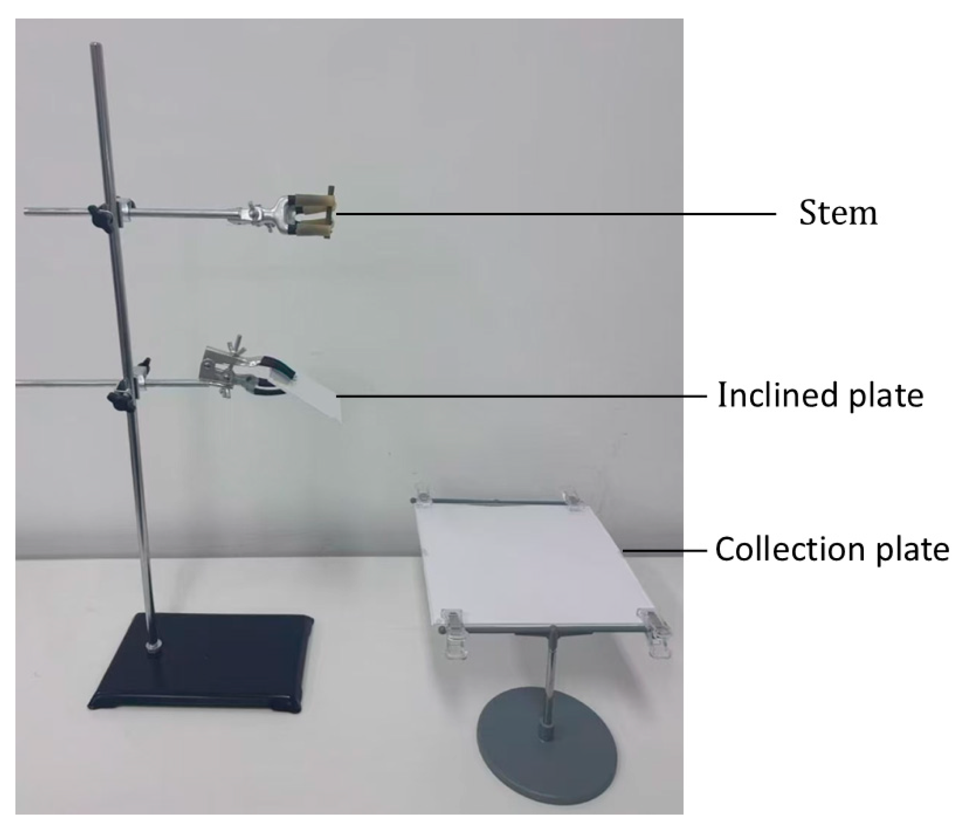
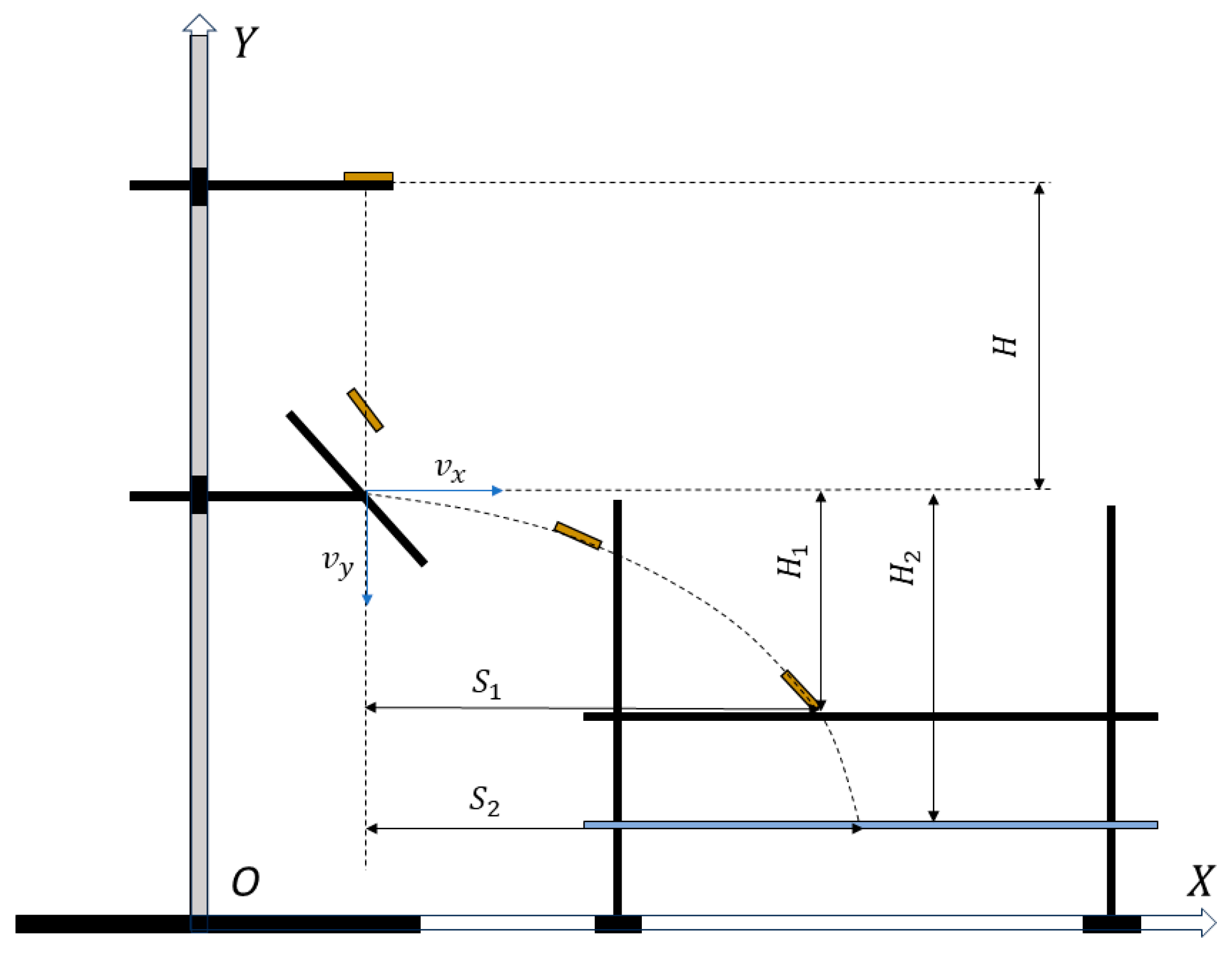
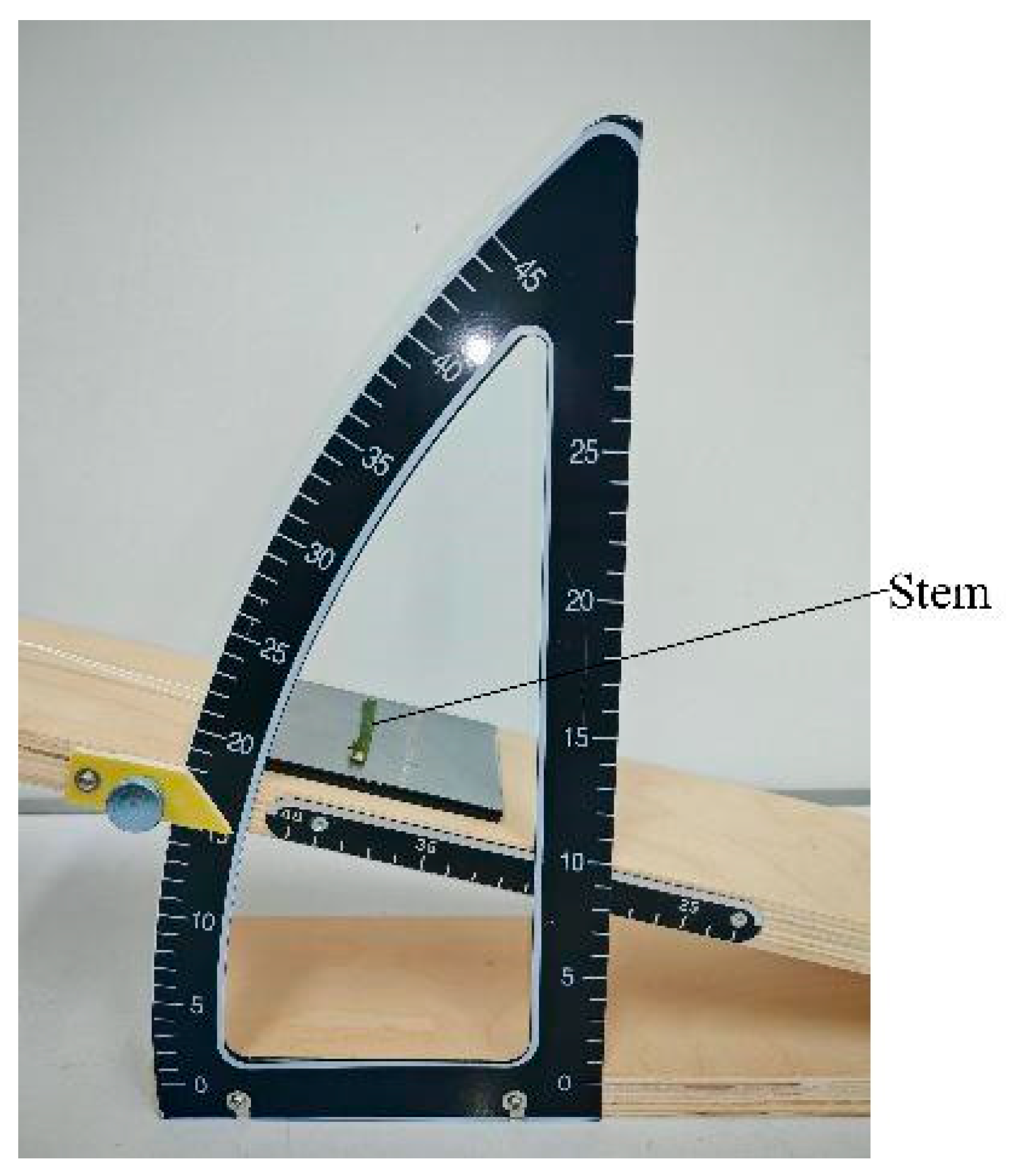
The coefficient of restitution was determined using a 45° inclined plate impact test [20]. The test device is shown in Figure 3, and its schematic diagram is shown in Figure 4. In this test, a tomato stem was raised to a height H of 300 mm above the acrylic plate and positioned to ensure a radial impact during free fall. Upon release, the stem underwent free fall, collided radially with the inclined plate, rebounded, and subsequently landed on a collection plate, producing a horizontal displacement S₁. The vertical distance between the impact point and the collection plate was recorded as H₁. The procedure was repeated by varying this vertical distance to H₂, and the corresponding horizontal displacement S₂ was measured.

The coefficient of restitution between the sample and the inclined plate was calculated using the following equation [21]:

$$e = {\displaystyle \frac{\sqrt{v_x^2+v_y^2}\cos \left({45}^{°}+\arctan \frac{v_y}{v_x}\right)}{v_0\sin {45}^{°}}}$$

(2)

$$\left\{\begin{array}{c}{\nu }_x=\sqrt{{\displaystyle \frac{g{S}_1{S}_2\left(S_1-S_2\right)}{2\left(H_1{S}_2-H_2{S}_1\right)}}}\\ {\nu }_y={\displaystyle \frac{H_1{\nu }_x}{S_1}}-{\displaystyle \frac{g{S}_1}{2{\nu }_x}}\end{array}\right.$$

(3)

where $v_0$, vertical velocity component before collision (m/s); ${\nu }_x$, horizontal velocity component after collision (m/s); ${\nu }_y$, vertical velocity component after collision (m/s); $g$, gravitational acceleration (m/s²).

The test was repeated ten times, and the data were recorded. The average value of the coefficient of restitution was determined from the calculations.

For the static friction coefficient measurement, the alloy steel plate was fixed on the inclined surface is shown in Figure 5. A tomato stem sample was placed on the plate, and the inclination angle of the ramp was gradually increased until the stem initiated sliding. The critical angle was recorded as the static friction angle, and the static friction coefficient was derived using the standard conversion formula. For the dynamic friction coefficient measurement, the alloy steel plate was not fixed; instead, it was driven to move upward along the ramp at a constant speed of 10 mm/s, controlled by the motor controller with a speed control accuracy of ±0.1 mm/s. To ensure the constant-velocity requirement, a 200 fps high-speed camera FDC-HD200HE was employed to record the movement of the steel plate. Frame-by-frame analysis of the displacement-time relationship verified that the deviation from a constant velocity was less than 2%. During the test, when the tomato stem remained stationary relative to the moving inclined plane, the corresponding angle was recorded as the dynamic friction angle, and the dynamic friction coefficient was calculated accordingly. To minimize the influence of moisture content variations, all measurements were completed within a short timeframe. Each test was repeated ten times to determine the average friction coefficients between the tomato stems and the alloy steel plate.

Figure 5. Friction coefficient measurement device diagram.

Figure 5. Friction coefficient measurement device diagram.

2.2. Contact Model of Tomato Stem

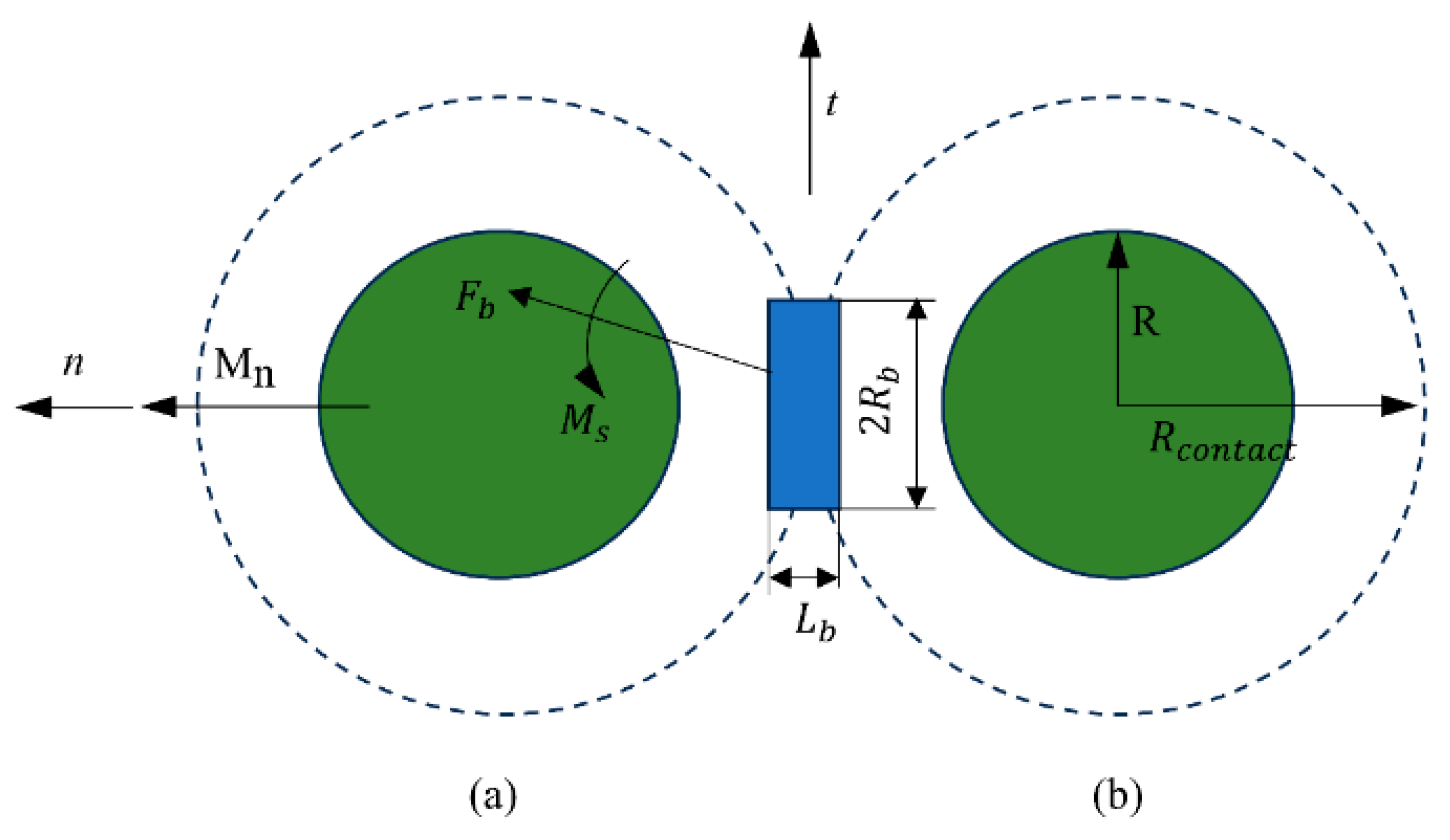
The discrete element model is composed of spherical particles. A Hertz-Mindlin contact model with bonding was employed to establish the tomato stem model. This modeling approach allows for the formation of bonding bonds between particles, enabling the simulation of the biomechanical properties of plant stems through the formation and breakage of these bonds. A schematic diagram of the bonding bonds between particles is presented in Figure 6.

In the diagram, F_b represents the resultant force exerted by Particle A on Particle B; M_n and M_s denote the normal and tangential moments, respectively; n and t are the unit vectors in the normal and tangential directions, respectively; L_b is the overlap between Particle A and Particle B; R_b is the bonding radius; R is the particle radius; and R_contact is the contact radius. To ensure sufficient connection between particles, the contact radius R_contact is set to be 20% to 30% larger than the particle radius R. The forces and moments acting on a particle are calculated using the following equations:

$$\delta F_n = v_n{k}_b^n{A}^{\prime }{\delta }_t$$

(4)

$$\delta F_t=v_t{k}_b^s{A}^{\prime }{\delta }_t$$

(5)

$$\delta M_n={\omega }_n{k}_b^{s}J{\delta }_t$$

(6)

$$\delta M_s={\omega }_t{k}_b^{n}J{\delta }_t ∕2$$

(7)

where A′, contact area (mm²); k_bⁿ, normal stiffness per unit area (N/m³); k_b^s, shear stiffness per unit area (N/m³); δ_t, time step (s); v_n, v_t, normal and tangential velocities (m/s); ω_n, ω_t, normal and tangential angular velocities (rad/s); δM_n, δM_s, incremental normal and tangential moments (N·m); δF_n, δF_t, incremental normal and tangential cohesive forces (N); J, moment of inertia (mm⁴).

The tangential and normal forces between particles act on the bonding bond. Due to particle motion (translation or rotation), the bond fractures when the stress exceeds a predefined threshold, according to the following criteria [22]:

$${\sigma }_{max} < {\displaystyle \frac{-F_n}{A^{\prime }}} + {\displaystyle \frac{2M_t}{J}}{R}_b$$

(8)

$${\tau }_{max} < {\displaystyle \frac{-F_t}{A^{\prime }}}+{\displaystyle \frac{2M_n}{J}}{R}_b$$

(9)

where $\sigma$_max, critical normal stress (Pa); τ_max, critical shear stress (Pa); R_b, bonding radius (m).

2.3. Tomato Stem Model Construction

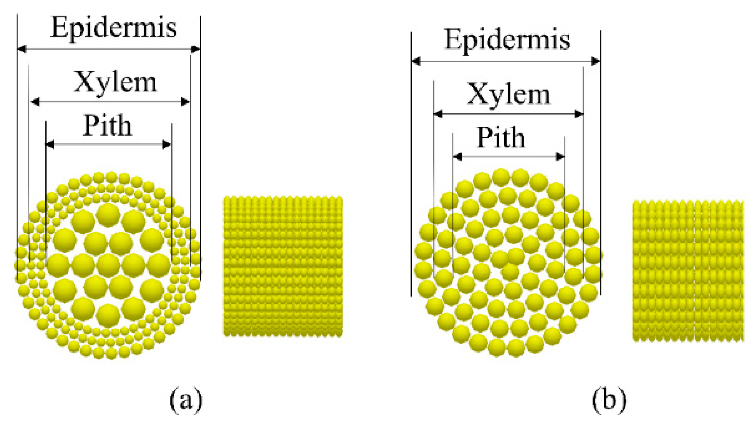
Through microscopic observation and measurement of the cross-sections of 7.5 mm-diameter tomato stems, it was found that the epidermis accounts for a small proportion of approximately 15%, about 1 mm in diameter, exhibits low structural strength [23]; the xylem accounts for a relatively large proportion of approximately 20%, about 1.5 mm in diameter and features high structural strength [24]; the pith is heterogeneous with soft internal cancellous tissue and constitutes the largest proportion of approximately 65%, about 5 mm in diameter. To simplify the stem discrete element model and improve computational efficiency, one approach is to scale up the internal structural dimensions of the stem and represent the internal structures with identical particles, albeit at the cost of reduced model accuracy. In contrast, filling the stem model with different types of particles renders its biomechanical properties more consistent with those of actual plant stems. Therefore, in the discrete element model, three components, namely the epidermis, xylem and pith, were separately filled with particles of different sizes to construct the model of a 7.5 mm-diameter tomato stem. The diameters of particles for the three components were 0.5 mm, 0.375 mm and 1 mm, respectively. Among them, medium-sized particles of 0.5 mm were used to fill the epidermis. Given the small proportion and low structural strength of the epidermis, the application of medium-sized particles can reduce the particle count in this region, improve computational efficiency, and simultaneously reflect the loose structure and low-strength mechanical properties of the epidermis. Small particles of 0.375 mm were adopted to fill the xylem. Owing to the relatively large proportion and high structural strength of the xylem, the smallest particles can accurately simulate the dense tissue structure of the xylem and precisely characterize its mechanical properties of high strength and high stiffness. Large particles of 1 mm were utilized to fill the pith. As the pith accounts for the largest proportion but features soft internal tissue, the use of medium-sized particles can balance computational accuracy and efficiency while reflecting the loose and porous tissue characteristics of the pith. The resulting tomato stem discrete element model comprises 18,018 particles and generates 79,286 bonding bonds. To evaluate the effect of the bond enhancement, a traditional model was constructed in parallel to serve as a baseline for comparison, as shown in Figure 7.

2.4. Bonding Parameter Calibration with Initial Values

A shear simulation test of tomato stems was conducted with shear force as the target response. A two-level factorial design was first employed to screen for factors exerting significant effects on the shear force. This was followed by a steepest ascent experiment to determine the optimal region of these significant factors. Finally, response surface methodology was applied to establish a regression model for the significant factors, leading to the identification of the optimal parameter combination.

The key parameters governing the bonding bonds between particles in the Hertz-Mindlin with Bonding contact model include the normal stiffness Kn, tangential stiffness Ks, critical normal stress σ, critical tangential stress τ, and bonding radius R_j [25,26]. These parameters are governed by the following equations:

$$\left\{\begin{array}{c}{K}_n={\displaystyle \frac{4}{3}}{\left({\displaystyle \frac{1-{\epsilon }_a^2}{E_a}}+{\displaystyle \frac{1-{\epsilon }_b^2}{E_b}}\right)}^{-1}{\left({\displaystyle \frac{r_a+r_b}{r_a{r}_b}}\right)}^{-{\displaystyle \frac{1}{2}}}\\ K_s={\displaystyle \frac{2}{3}}{K}_n\\ \sigma ={\displaystyle \frac{F}{\pi R^2}}\\ \tau =c+\sigma \tan \phi \end{array}\right.$$

(10)

where ${\epsilon }_a$, ${\epsilon }_b$, Poisson’s ratio of particles; $E_a$, $E_b$, Elastic modulus of particles (MPa); $r_a$, $r_b$, Particle radius (mm); $R$, Radius of the compression surface (mm); $c$, Cohesion of the stem material (MPa); $\phi$, Internal friction angle (degree).

The bonding parameters were preliminarily estimated through theoretical calculation. These parameters were designated as the experimental factors x₁ to x₂₀ for a two-level factorial design, as listed in

Table 1. Factors of the two-level factorial experiment.

	Pith-Pith	Pith-Xylem	Xylem- Xylem	Xylem- Epidermis	Epidermis-Epidermis
Kn/N·m−3	x1 = 3.4 × 107	x2 = 4.2 × 107	x3 = 2 × 108	x4 = 8.4 × 107	x5 = 6.4 × 107
Ks/N·m−3	x6 = 2.3 × 107	x7 = 2.8 × 107	x8 = 1.3 × 108	x9 = 5.6 × 107	x10 = 4.3 × 107
$\sigma$/Pa	x11 = 3.6 × 106	x12 = 4 × 107	x13 = 4 × 107	x14 = 8.4 × 106	x15 = 8.4 × 106
$\tau$/Pa	x16 = 1.2 × 107	x17 = 3.2 × 107	x18 = 3.2 × 107	x19 = 1.6 × 107	x20 = 1.6 × 107

. The bonding radius R_j was additionally set as factor x₂₁ = 3.25 × 10⁻⁴ m. The calculated values for all factors were coded from X₁ to X₂₁ and maintained at their center points. A high level and a low level were then assigned to each factor, corresponding to an increase and a decrease of approximately 20% from its central value, respectively. In the two-level factorial design, ±20% is adopted as the standard perturbation magnitude for sensitivity analysis. An excessively small amplitude results in insignificant effects, while an overly large one readily triggers nonlinear coupling or numerical instability [27].

2.5. Two-Level Factorial Design and Steepest Ascent Test

The coded factors X₁ to X₂₁ were assigned high and low levels for the two-level factorial experiment. With the shear force of the tomato stem set as the target response for the simulation, a two-level factorial design comprising 32 simulation trials was constructed. This design effectively screened for the parameters exerting the most significant influence on the shearing force.

Based on the results of the factorial experiment, the parameters identified as having a significant effect on shear force were selected for a subsequent steepest ascent test. All non-significant factors were fixed at their central level. Six trial points were arranged along the path of steepest ascent. As the levels of the significant factors were systematically adjusted, the simulated shear force changed accordingly. The trial point yielding a shear force closest to the experimentally measured value was identified. The factor levels from this point and its adjacent predecessor were then designated as the low and high levels, respectively, for the subsequent Box–Behnken design.

2.6. Box–Behnken Experiment

To obtain the optimal combination of bonding parameters, with shear force as the response variable, a three-factor, three-level Box–Behnken response surface design was conducted using Design-Expert 13 software. Each experimental run was replicated 20 times, and the average value of the measured shear force was used as the response, based on the results from the previous two-level factorial and steepest ascent tests [28,29]. The results of the response surface experiments were analyzed and fitted to establish a second-order regression model describing the relationship between shear force and the influencing factors. A comprehensive analysis of the Box–Behnken response surface results was subsequently performed.

3. Results

3.1. Experimental Results of Stem Model Parameter Testing

Shear tests were performed on tomato stems with a diameter of 7.5 mm. Five replicate tests yielded an average shearing force of 28.9 N. The results of the intrinsic parameter tests were as follows: density ρ = 960.5 kg·m⁻³, Poisson’s ratio μ = 0.34, and shear modulus G = 3.4 × 10⁷ Pa. The results of the contact parameter tests are summarized in

Table 2. Tomato stem contact parameters.

Contact Materials	Parameter	Mean Value
Tomato Stem—Tomato Stem	Coefficient of Restitution	0.41
	Static Friction Coefficient	0.56
	Rolling Friction Coefficient	0.24
Tomato Stem—Alloy Steel	Coefficient of Restitution	0.51
	Static Friction Coefficient	0.62
	Rolling Friction Coefficient	0.28

.

3.2. Results of the Two-Level Factorial and Steepest Ascent Tests

The analysis of variance for the two-level factorial design identified factors with p-values less than 0.01, as summarized in

Table 3. Analysis of Variance (ANOVA) for screening significant bonding parameters affecting tomato stem shear force.

Source of Variation	F/N
	Mean Square	DF	Sum of Squares	F Value	p Value
Model	10.116	21	212.429	27.920	<0.001
X3	191.590	1	191.590	528.799	<0.001
X8	7.315	1	7.315	20.191	<0.001
X21	9.790	1	9.790	27.022	<0.001

. As shown in the table, the model’s p-value is far below 0.05, indicating that the results are statistically significant. Specifically, the coded factors X₃ (normal stiffness of xylem-xylem contact), X₈ (tangential stiffness of xylem-xylem contact), and X₂₁ (particle bonding radius) all have p-values less than 0.01. This demonstrates that the corresponding parameters—xylem-xylem normal stiffness (x₃), xylem-xylem tangential stiffness (x₈), and particle bonding radius (x₂₁)—exert a significant influence on the shear force. In contrast, the effects of the remaining factors were negligible.

Based on the results of the two-level factorial design, the parameters that exhibited a significant influence on the shear force of the tomato stem—namely X₃, X₈, and X₂₁—were selected for the steepest ascent test. All non-significant factors were held constant at their central level. The experimental design and results are presented in

Table 4. Scheme and results of steepest ascent test.

No.	Factor			F/N
	${\mathit{x}}_3$/$(\mathbf{N}·{\mathbf{m}}^{-3})$	${\mathit{x}}_8$/$(\mathbf{N}·{\mathbf{m}}^{-3})$	${\mathit{x}}_{21}$/$\mathbf{m}$
1	$2\times {10}^8$	$1.3\times {10}^8$	$3.25\times {10}^{-4}$	27.4
2	$2.4\times {10}^8$	$1.56\times {10}^8$	$3.30\times {10}^{-4}$	29.8
3	$2.8\times {10}^8$	$1.82\times {10}^8$	$3.35\times {10}^{-4}$	32.3
4	$3.2\times {10}^8$	$2.08\times {10}^8$	$3.40\times {10}^{-4}$	33.9
5	$3.6\times {10}^8$	$2.34\times {10}^8$	$3.45\times {10}^{-4}$	36.2
6	$4\times {10}^8$	$2.6\times {10}^8$	$3.50\times {10}^{-4}$	38.5

. As the levels of these factors increased incrementally along the steepest ascent path, the simulated shear force of the tomato stem gradually increased. This trend can be attributed to the underlying bonding mechanics in the Hertz-Mindlin with Bonding contact model: higher normal and tangential stiffness values enhance the resistance of bonding bonds to deformation under external loads, thereby delaying the onset of bond failure. According to the bond failure criterion, the critical normal and tangential forces that a bond can sustain are proportional to both the critical stress and the effective bonding area. Consequently, increasing the bonding radius directly expands the effective cohesive area, requiring greater external shear force to reach the critical stress threshold for bond rupture. Specifically, the shear forces recorded for Trial 1 and Trial 3 were 27.4 N and 32.3 N, respectively. The factor levels corresponding to Trial 1 and Trial 3 were subsequently designated as the low and high levels for the ensuing Box–Behnken experimental design.

3.3. Results of the Box–Behnken Experiment

To obtain the optimal combination of bonding parameters, the experimental design and corresponding results are presented in

Table 5. Box–Behnken Experimental Design and Results.

No.	X3	X8	X21	F/N
1	−1	−1	0	28.2
2	0	0	0	29.8
3	0	−1	−1	29.3
4	1	−1	0	32.3
5	1	0	−1	31.6
6	1	1	0	31.7
7	−1	0	−1	27.9
8	0	−1	1	30.7
9	0	0	0	29.8
10	1	0	1	32.2
11	−1	1	0	28.1
12	0	0	0	29.8
13	0	1	−1	29.1
14	−1	0	1	28.4
15	0	1	1	30.5

, where each F/N value represents the average of 20 replicate measurements. Based on the analysis and fitting of the Box–Behnken experiment results, a second-order regression model describing the relationship between shear force and the influencing factors was established as follows:

F = 29.8 + 1.9X3 + 0.0625X8 + 0.2875X21 − 0.125X3X8 + 0.025X3X21 + 0.4X8X21 + 0.4X32 − 0.125X82 − 0.175X212

(11)

where X₃ is the normal stiffness of xylem-xylem contact coded factor, with natural units ranging from 2.0 × 10⁸ N⋅m⁻³ (low level, −1) to 2.8 × 10⁸ N⋅m⁻³ (high level, +1), and a center level of 2.4 × 10⁸ N⋅m⁻³; X₈ is the tangential stiffness of xylem-xylem contact (coded factor), with natural units ranging from 1.3 × 10⁸ N⋅m⁻³ (low level, −1) to 1.82 × 10⁸ N⋅m⁻³ (high level, +1), and a center level of 1.56 × 10⁸ N⋅m⁻³; X₂₁ is the particle bonding radius (coded factor), with natural units ranging from 3.25 × 10⁻⁴ m (low level, −1) to 3.35 × 10⁻⁴ m (high level, +1), and a center level of 3.30 × 10⁻⁴ m.

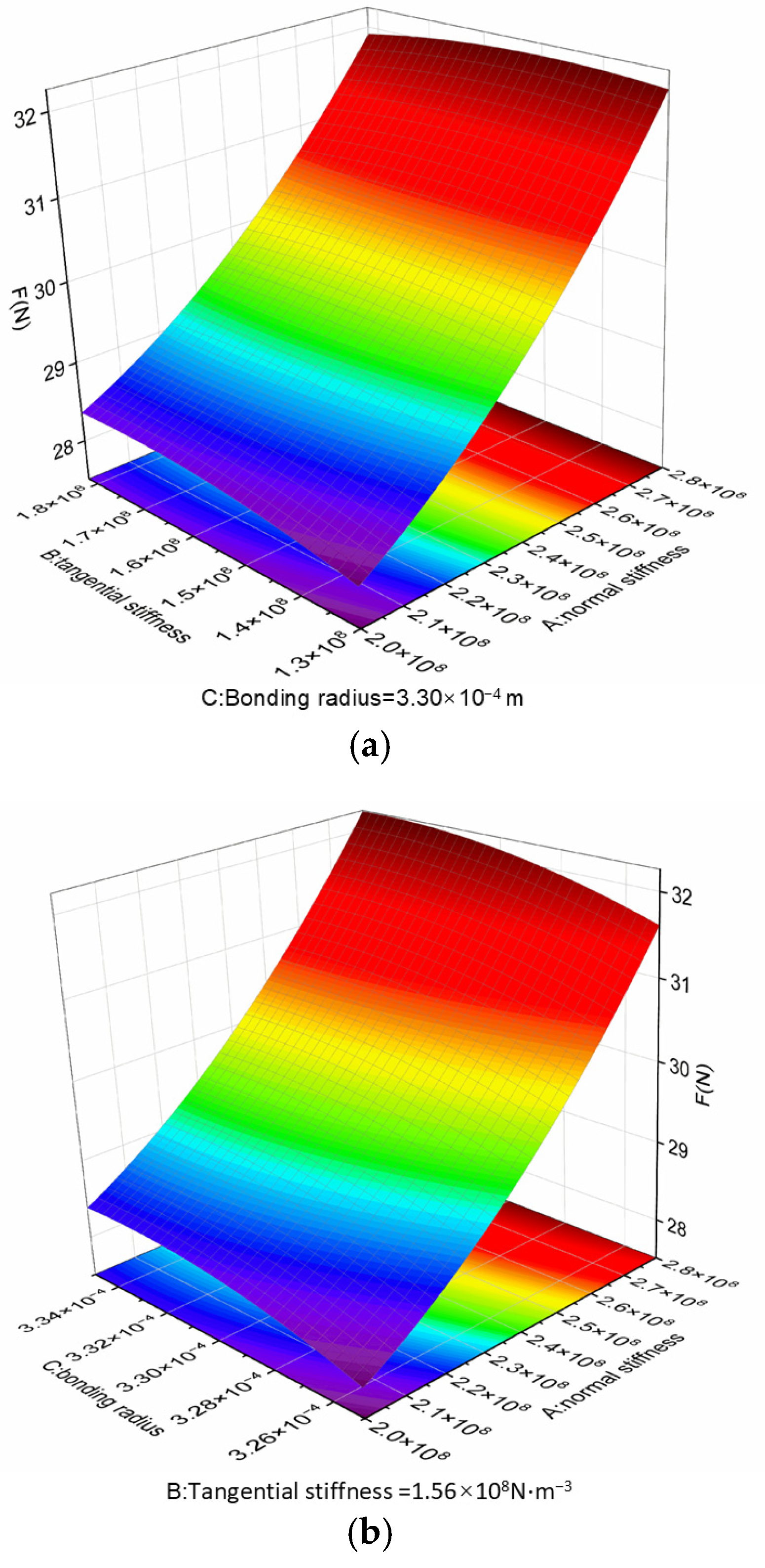
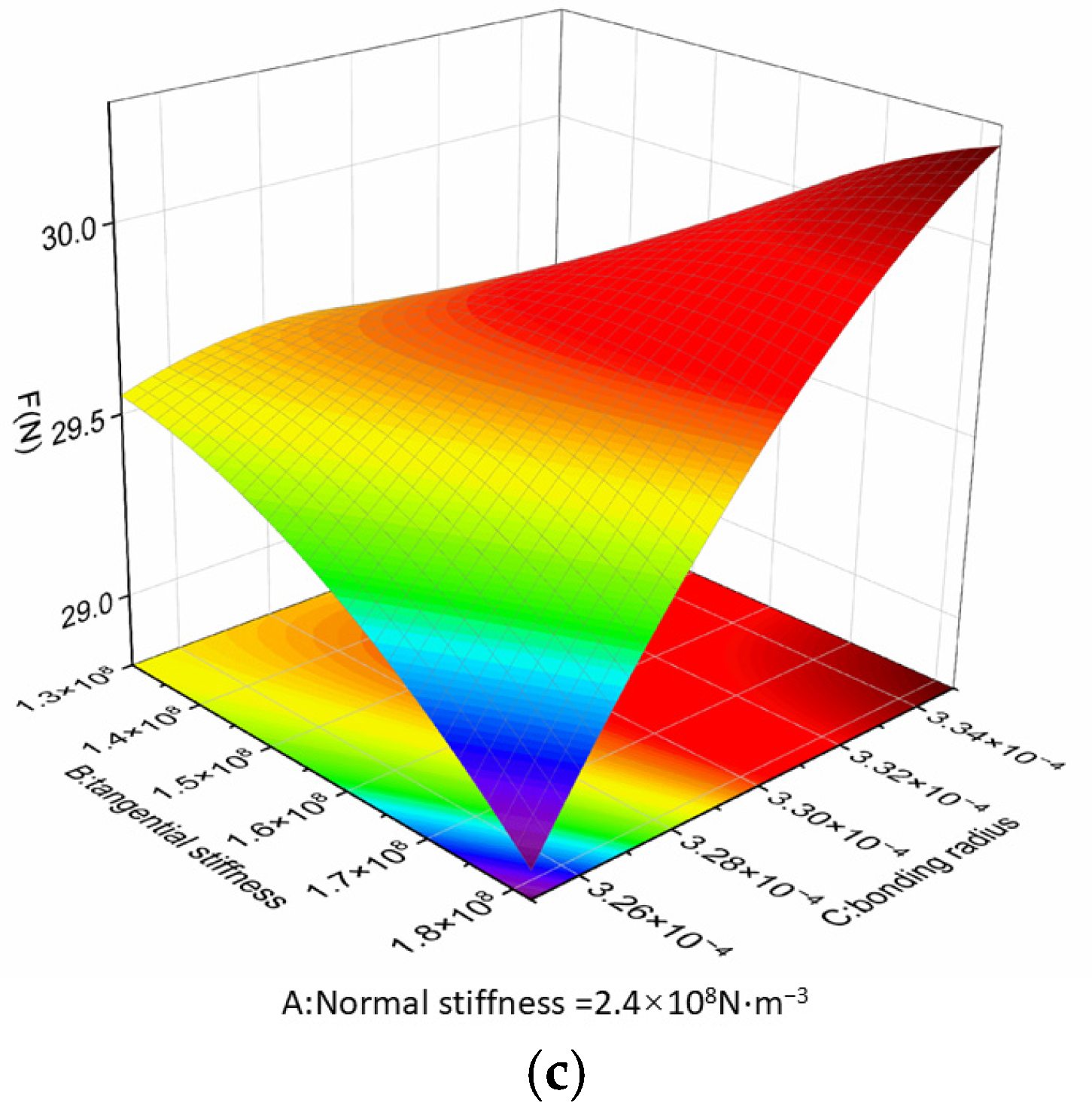
An analysis of variance was performed on the Box–Behnken design, and the results are presented in

Table 6. ANOVA for Box–Behnken results.

Source of Variation	F/N
	MS	DF	F	p
Model	31.104	9	52.88	0.0001
X3	28.88	1	441.879	0.0001
X8	0.031	1	0.478	0.511
X21	0.661	1	10.117	0.015
X3  X 8	0.062	1	0.956	0.36
X3  X 21	0.002	1	0.038	0.85
X8  X 21	0.64	1	9.792	0.016
X32	0.673	1	10.307	0.014
X82	0.065	1	1.006	0.349
X212	0.128	1	1.972	0.202
Residual	0.457	7
Lack of Fit	0.457	3
Pure Error	0	4
R2 = 0.986

. As shown in Table 6, the second-order regression model has a coefficient of determination (R²) of 0.986, indicating an excellent fit. The model itself is statistically significant, while the lack-of-fit term is not significant. This suggests that the model adequately captures the relationship within the experimental domain and that no other major factors unaccounted for significantly influence the response value. The factor X₃ has a p-value of less than 0.01, the factor X₂₁, the interaction term X₈X₂₁, and the quadratic term X₃² all have p-values less than 0.05, indicating a significant influence. The effects of the remaining terms are not statistically significant. Response surface plots illustrating the interactive effects of these significant factors on the shearing force are presented in Figure 8.

As shown in Figure 8, when the bonding radius x₂₁ was fixed at 3.30 × 10⁻⁴ m, the shearing force reached its minimum value of 28.1 N at a normal stiffness x₃ of 2 × 10⁸ N⋅m⁻³ and a tangential stiffness x₈ of 1.82 × 10⁸ N⋅m⁻³. The shear force increased with increasing normal stiffness x₃ and decreasing tangential stiffness x₈, reaching its maximum value of 32.3 N when x₃ was 2.8 × 10⁸ N⋅m⁻³ and x₈ was 1.3 × 10⁸ N⋅m⁻³. With the tangential stiffness x₈ fixed at 1.56 × 10⁸ N⋅m⁻³, the shearing force exhibited a minimum of 27.9 N at a normal stiffness x₃ of 2.8 × 10⁸ N⋅m⁻³ and a bonding radius x₂₁ of 3.25 × 10⁻⁴ m. The shear force increased with simultaneous increases in both normal stiffness x₃ and bonding radius x₂₁, achieving a maximum of 32.2 N when x₃ was 2.8 × 10⁸ N⋅m⁻³ and x₂₁ was 3.35 × 10⁻⁴ m. When the normal stiffness x₃ was held constant at 2.4 × 10⁸ N⋅m⁻³, the shear force increased with concurrent increases in both tangential stiffness x₈ and bonding radius x₂₁. The maximum shear force under this condition was 30.5 N, observed at x₂₁ = 3.35 × 10⁻⁴ m.

3.4. Optimal Parameter Combination and Validation

Using the actual shear force of the tomato stem as the target response, the fitted regression equation was solved to obtain the optimal combination of the statistically significant parameters: normal stiffness x₃ = 2.05 × 10⁸ N⋅m⁻³, tangential stiffness x₈ = 1.62 × 10⁸ N⋅m⁻³, and bonding radius x₂₁ = 3.26 × 10⁻⁴ m. All remaining parameters were maintained at their central levels. A simulated shear test was conducted in EDEM using this optimal parameter set. For comparison, parallel simulations were performed using both a traditional tomato stem model and the pre-optimized model.

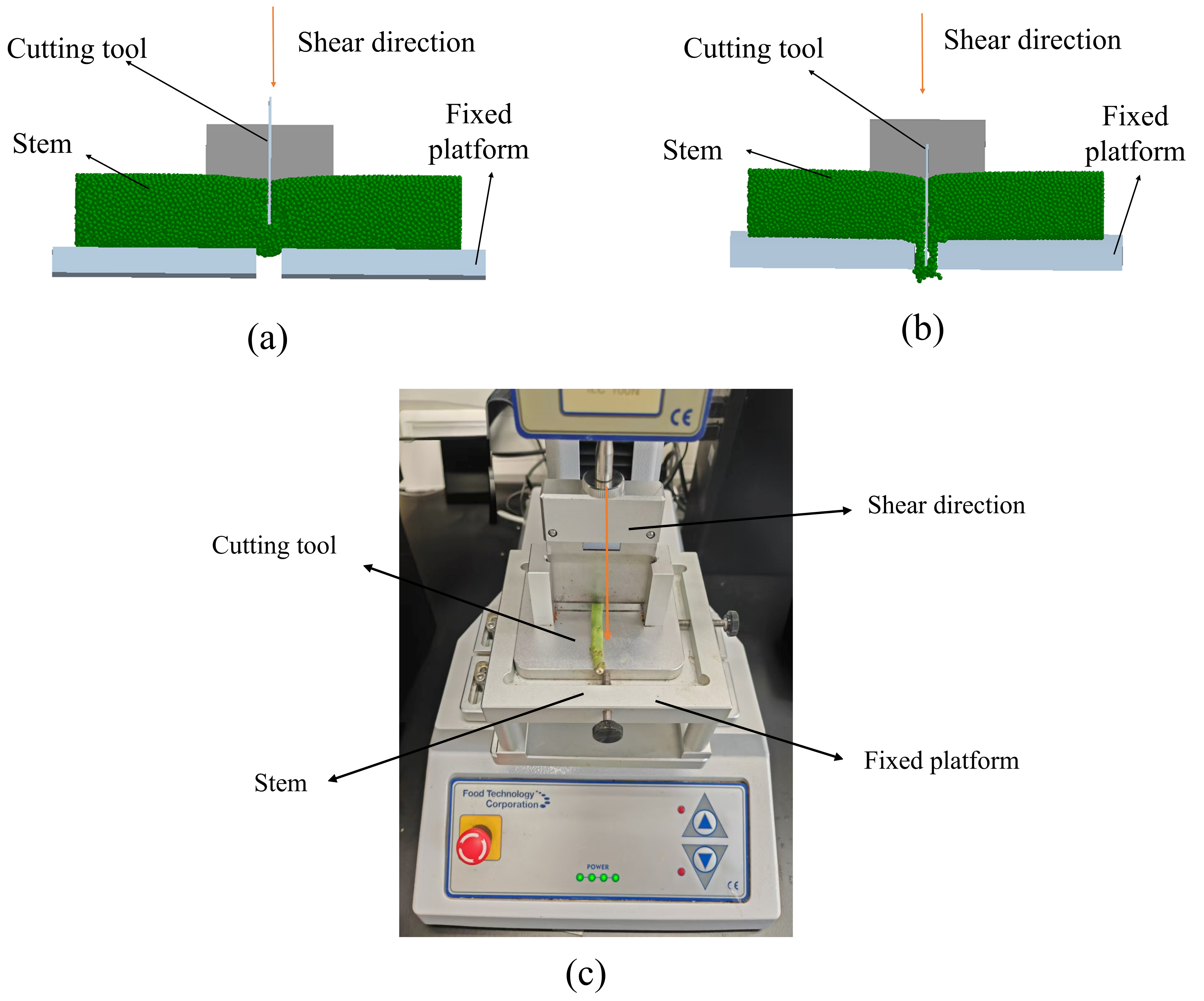
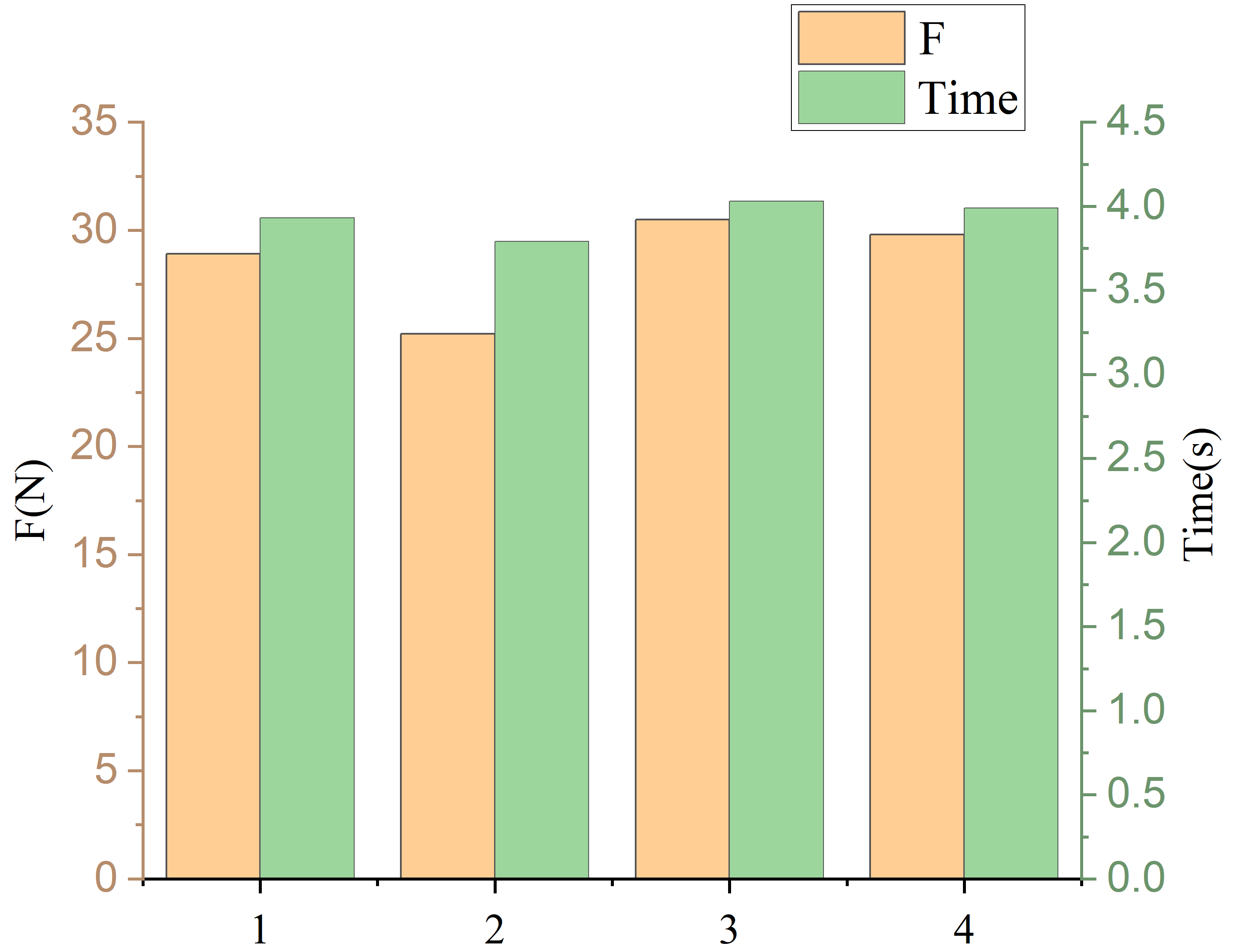
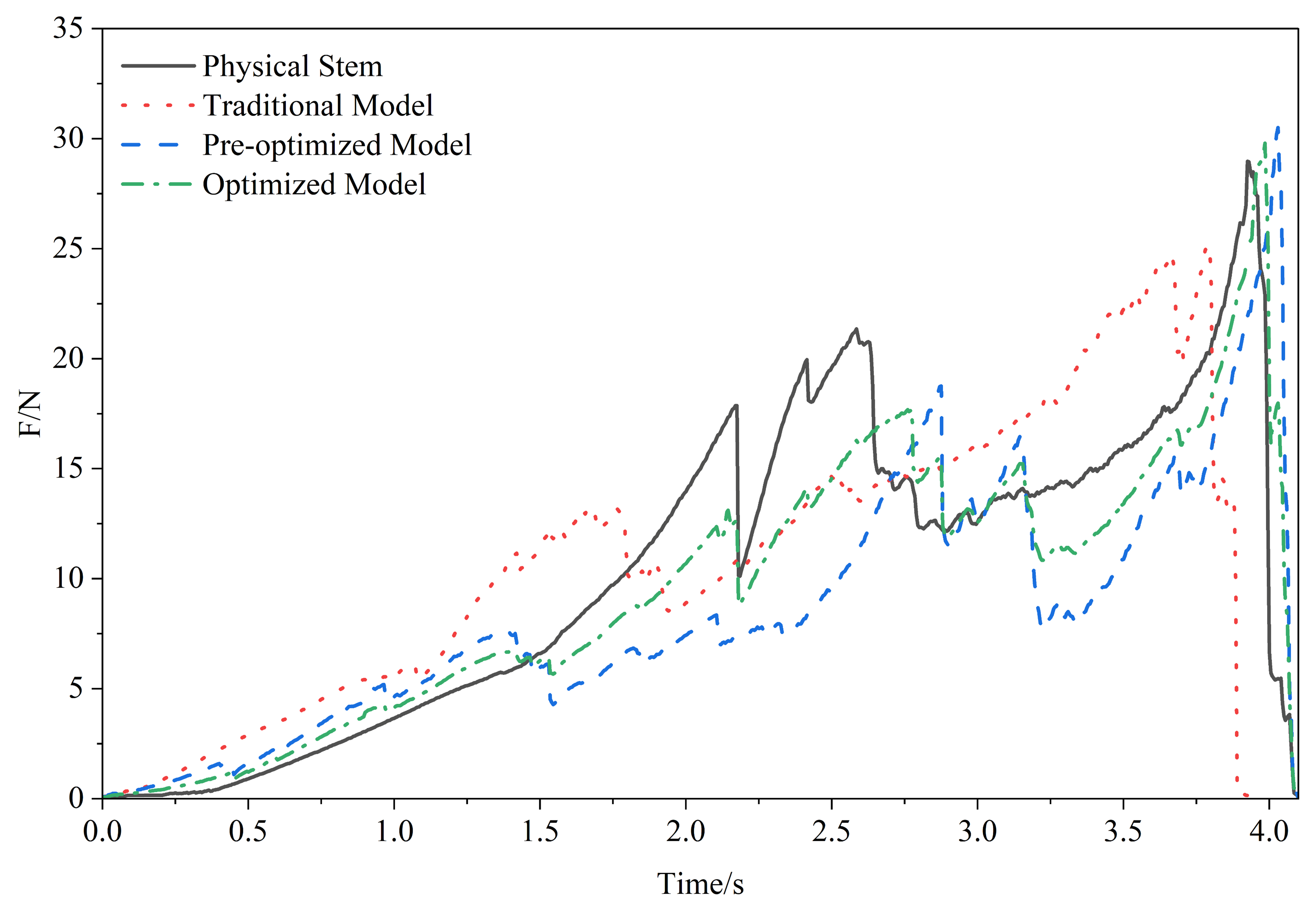
The simulated shearing process of the discrete element model alongside the physical shear test is illustrated in Figure 9. A comparison of the force–time curves obtained from the simulation and the physical experiment is presented in Figure 10. The force values and times for the peak are compared in Figure 11. As shown in Figure 11, the second peak force and time were: 28.9 N and 3.93 s for the physical test; 25.2 N and 3.79 s for the traditional model; 30.5 N and 4.03 s for the pre-optimized model; and 29.8 N and 3.99 s for the optimized model. Among these models, the optimized model presents the minimum relative error of the maximum shear force, which is 3.1%. Figure 10 presents the shear force–time curves derived from physical shear tests and corresponding discrete element method simulations of tomato stems. The shearing process of tomato stems proceeds sequentially from the upper to the lower portion: the cutting tool initially induces compressive deformation in the upper xylem, leading to a rapid rise in shear force until the upper xylem is fractured, which generates the first peak corresponding to the shear fracture force of the upper xylem; the tool then cuts into the soft pith, causing a transient decline in shear force, and after passing through the pith, it deforms the lower xylem, with the shear force increasing again until the lower xylem is completely sheared off, forming the maximum peak that represents the ultimate shear force of the whole stem. The optimized DEM can better reproduce these two peak features because small-sized particles are adopted to fill the xylem, which precisely characterizes the dense tissue structure and the high-strength, high-stiffness mechanical properties of the xylem, thus authentically restoring the deformation and fracture mechanisms of tomato stems during shearing.

The traditional model exhibited substantial errors in both response magnitude and response speed at the two shear force peaks compared to the physical tomato stem. The pre-optimized model also showed considerable error in the response speed and the maximum peak response value at the first peak. In contrast, the optimized model demonstrated significant improvement: it reduced the error in response speed at the first peak by 85.3% and 44.2% relative to the traditional and pre-optimized models, respectively. Furthermore, the errors in the maximum peak response value and the corresponding response speed were reduced by 75.8%, 43.7%, 58.3%, and 40%, respectively, compared to the two baseline models. These results indicate that the tomato stem model with the optimal parameter set achieves highly accurate simulation performance, confirming that the calibrated and optimized parameters are both reliable and effective.

4. Discussion

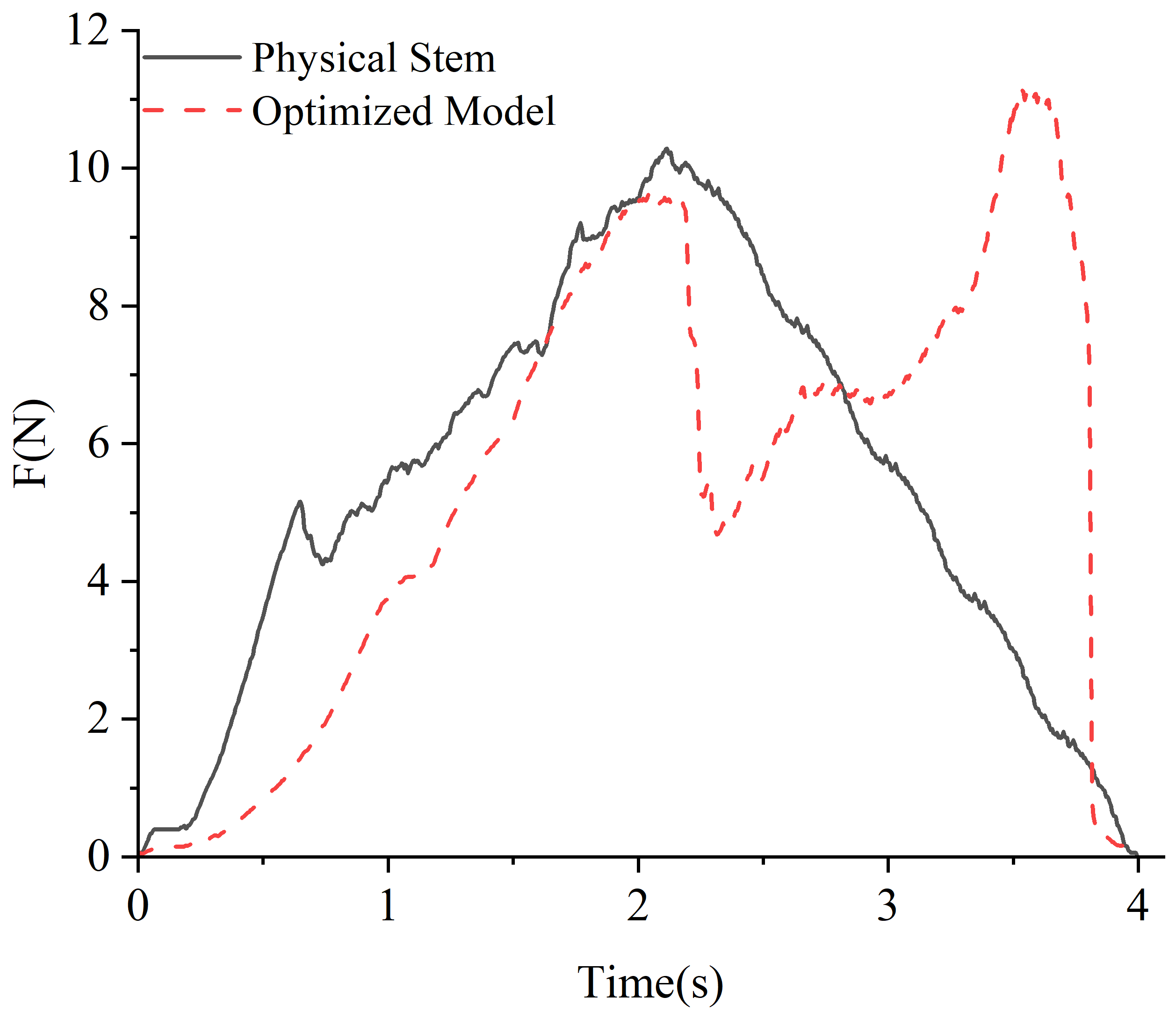
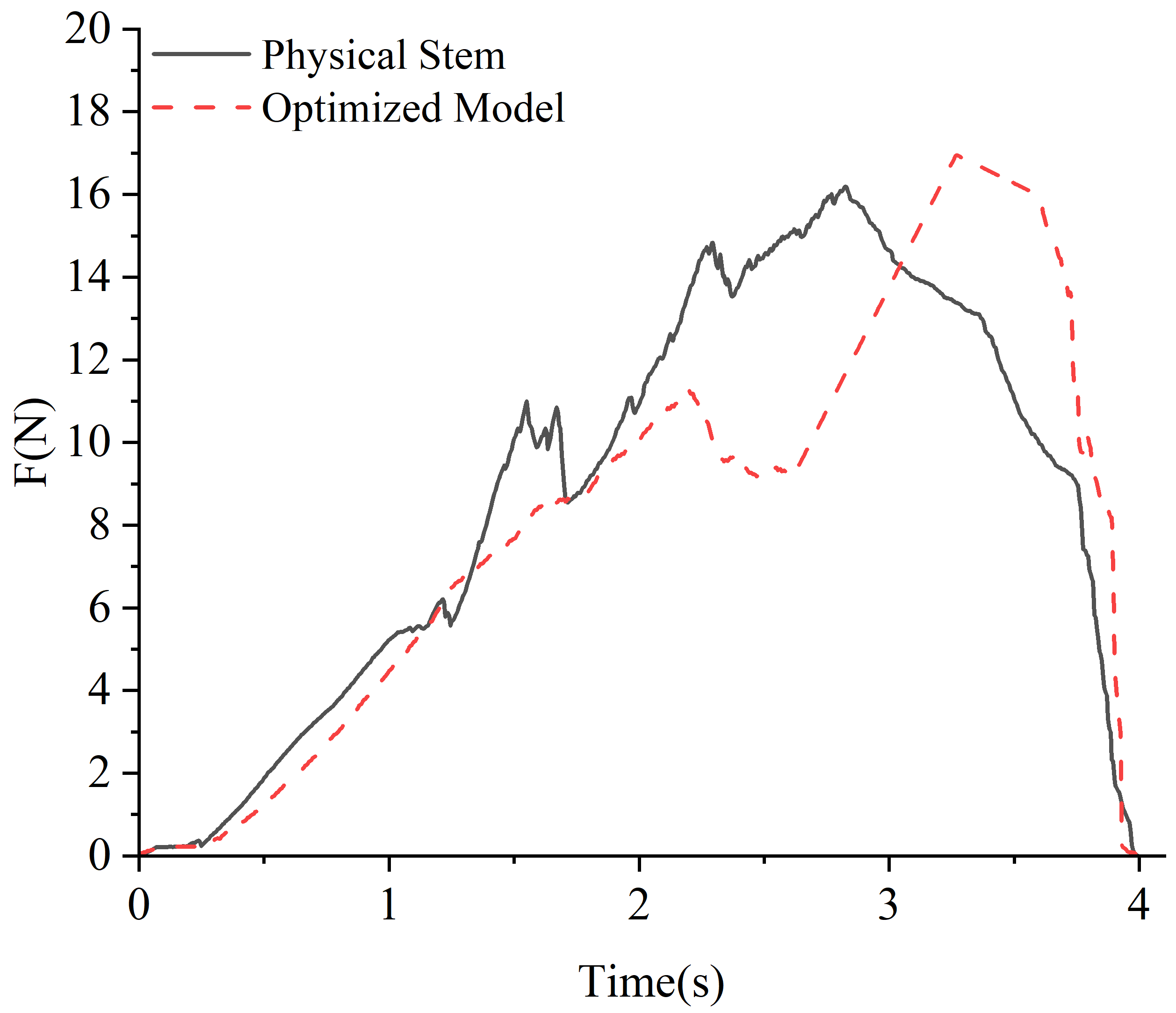
This section discusses the shear force–time curves obtained from physical tests of tomato stems with diameters of 3.5 mm, 5.5 mm, and 7.5 mm as well as the calibrated three-layer bonded discrete element model, and discusses the influence of xylem maturation on simulation accuracy. The shear force–time curves from physical tests of 3.5 mm and 5.5 mm tomato stems are presented in Figure 12 and Figure 13, respectively. For 3.5 mm-diameter tomato stems, the measured maximum shear force was 10.3 N, while the simulated value was 11.1 N, with a relative error of 7.8%; notably, the physical shear curve exhibited no double-peak characteristic, whereas the simulated curve still retained distinct double peaks, resulting in a large deviation in the force variation trend. This discrepancy can be attributed to the immature xylem of lateral branches with a diameter less than 5 mm, which possesses extremely low mechanical strength and fails to form a clear stratified structure with the epidermis and pith, thus eliminating the double-peak fracture behavior during shearing. For 5.5 mm-diameter tomato stems, the measured maximum shear force was 16.2 N, and the simulated value was 17.0 N, with a relative error reduced to 4.9%; meanwhile, the physical shear curve initially presented the double-peak feature, as the xylem gradually matured and provided sufficient structural strength, leading to a significantly improved matching degree between the simulated and measured shear force–time curves. For 7.5 mm-diameter tomato stems, the measured maximum shear force was 28.9 N, and the simulated value was 29.8 N, with a relative error as low as 3.1%; the fully matured xylem formed a distinct high-strength layered structure, and the simulated curve accurately reproduced the double-peak evolution law and peak values of the physical test, further enhancing the overall simulation accuracy.

The above results demonstrate that the simulation accuracy of the established DEM is positively correlated with the maturation degree of tomato stem xylem. Since the tomato stems targeted for pruning in production are mainly concentrated at diameters above 5.5 mm, the calibrated three-layer bonded DEM can meet the simulation requirements of stem shearing in actual pruning scenarios and provide reliable parameter support and a simulation basis for the design and optimization of tomato pruning robots. However, heterogeneous structures such as immature stems with diameters less than 5 mm and over-aged stems inevitably exist in the actual pruning process, and the current model cannot accurately characterize their mechanical properties and shear fracture behaviors. Therefore, subsequent research will focus on the parameter calibration and model optimization of tomato stems with heterogeneous structures, so as to improve the universality and adaptability of the discrete element simulation model in the whole process of tomato pruning.

Compared with the single-layer homogeneous DEMs for flax stems [8] and wheat straw [10], which typically reported simulation errors exceeding 10%, the three-layer bonded DEM in this study achieved a lower relative error of 3.1% for 7.5 mm-diameter tomato stems. This improvement is consistent with the findings of Xie et al. [12], who demonstrated that multi-layer models for rapeseed stems yielded higher accuracy than single-layer approaches.

5. Conclusions

This study proposed a tomato stem model along with a method for calibrating and optimizing its bonding parameters. The physical properties of the stem were determined through experimental measurements. To obtain ideal values for the bonding parameters, calibration and optimization were performed via a series of tests, and the applicability of the model under the optimal parameters was verified. Comparative experiments were finally conducted to validate the accuracy of the optimized model. The following conclusions were drawn from this investigation:

(a) For a 7.5 mm diameter tomato stem, the measured physical properties were: density = 960.5 kg/m³, Poisson’s ratio = 0.34, shear modulus = 3.4 × 10⁷ Pa, and shearing force = 28.9 N.

(b) After establishing the tomato stem model, a two-level factorial design was first used to screen for factors significantly affecting shear force. A steepest ascent test was then applied to narrow the calibration range of these significant parameters. Subsequently, a Box–Behnken design was employed to develop a mathematical regression model between the target response (shear force) and three test factors: xylem–xylem normal stiffness, xylem–xylem tangential stiffness, and bond radius. Analysis of variance revealed the influence and interactions of these factors on shear force. The optimal parameter combination was determined as follows: normal stiffness x₃ = 2.05 × 10⁸ N·m⁻³, tangential stiffness x₈ = 1.62 × 10⁸ N·m⁻³, and bond radius x₂₁ = 3.26 × 10⁻⁴ m.

(c) In comparative shear tests, the measured shear forces for the physical stem, the traditional model, the pre-optimized model, and the optimized model were 28.9 N, 25.2 N, 30.5 N, and 29.8 N, respectively. The results show that the optimized model reduces the error in shear force by 75.8% and 43.7% compared to the traditional and pre-optimized models, demonstrating high simulation accuracy and confirming the reliability of the optimal parameter set.

In practical applications, the calibrated three-layer bonded DEM can be utilized to optimize the structural design of pruning end-effectors and minimize mechanical damage to tomato plants during automated pruning operations. Future research will focus on the parameter calibration and model optimization of tomato stems with heterogeneous structures to improve the universality and adaptability of the discrete element simulation model throughout the whole pruning process.

References

1. Idama, O.; Uguru, H. Robotization of tomato fruits production to enhance food security. J. Eng. Res. Rep. 2021, 20, 67–75. [Google Scholar] [CrossRef] [Scilit]
2. Appolloni, E.; Paucek, I.; Pennisi, G.; Manfrini, L.; Gabarrell, X.; Gianquinto, G.; Orsini, F. Winter greenhouse tomato cultivation: Matching leaf pruning and supplementary lighting for improved yield and precocity. Agronomy 2023, 13, 671. [Google Scholar] [CrossRef] [Scilit]
3. Feng, Q.; Cheng, W.; Li, Y.; Wang, B.; Chen, L. Method for identifying tomato plants pruning point using Mask R-CNN. Trans. Chin. Soc. Agric. Eng. 2022, 38, 128–135. [Google Scholar] [CrossRef]
4. Wang, B.; Zhang, W.; Feng, Q. Design and experiment of cutting type tomato pruning operation actuator. J. Agric. Mech. Res. 2024, 46, 53–59, 65. [Google Scholar] [CrossRef]
5. Zeng, Z.; Ma, X.; Cao, X.; Li, Z.; Wang, X. Critical review of applications of discrete element method in agricultural engineering. Trans. Chin. Soc. Agric. Mach. 2021, 52, 1–20. [Google Scholar] [CrossRef]
6. Wang, B.; Zhang, W.; Feng, Q. Measurement and analysis of mechanical properties of stem clamping for automatic pruning of tomato. J. Agric. Mech. Res. 2023, 45, 157–163. [Google Scholar] [CrossRef]
7. Yuan, J.; Li, J.; Zou, L.; Liu, X. Optimal design of spinach root-cutting shovel based on discrete element method. Trans. Chin. Soc. Agric. Mach. 2020, 51, 85–98. [Google Scholar] [CrossRef]
8. Shi, R.; Dai, F.; Zhao, W.; Zhang, F.; Shi, L.; Guo, J. Establishment of discrete element flexible model and verification of contact parameters of flax stem. Trans. Chin. Soc. Agric. Mach. 2022, 53, 146–155. [Google Scholar] [CrossRef]
9. Liao, Y.; Liao, Q.; Zhou, Y.; Wang, Z.; Jiang, Y.; Liang, F. Parameters calibration of discrete element model of fodder rape crop harvest in bolting stage. Trans. Chin. Soc. Agric. Mach. 2020, 51, 73–82. [Google Scholar] [CrossRef]
10. Schramm, M.; Tekeke, M.Z. Wheat straw direct shear simulation using discrete element method of fibrous bonded model. Biosyst. Eng. 2022, 213, 1–12. [Google Scholar] [CrossRef] [Scilit]
11. Liu, W.; Su, Q.; Fang, M.; Zhang, J.; Zhang, W.; Yu, Z. Parameters calibration of discrete element model for corn straw cutting based on Hertz-Mindlin with bonding. Appl. Sci. 2023, 13, 1156. [Google Scholar] [CrossRef] [Scilit]
12. Xie, W.; Peng, L.; Jiang, P.; Meng, D.; Wang, X. Discrete element model building and optimization of double-layer bonding of rape shoots stems at harvest stage. Trans. Chin. Soc. Agric. Mach. 2023, 54, 112–120. [Google Scholar] [CrossRef]
13. Zou, S.; Su, G.; Shao, Y.G. Simulation optimization and experiment of separation device for ramie stalks based on discrete element method. J. Chin. Agric. Mech. 2017, 38, 60–67. [Google Scholar] [CrossRef]
14. Han, D.; Wang, Q.; Tang, C.; Li, W.; Xu, Y. Calibration of the contact parameters for soybean bonded particle model based on discrete element method. J. Mech. Sci. Technol. 2025, 39, 1279–1287. [Google Scholar] [CrossRef] [Scilit]
15. Li, D.; Wang, R.; Zhu, Y.; Chen, J.; Zhang, G.; Wu, C. Calibration of simulation parameters for fresh tea leaves based on the discrete element method. Agriculture 2024, 14, 148. [Google Scholar] [CrossRef] [Scilit]
16. Coetzee, C. Calibration of the discrete element method: Strategies for spherical and non-spherical particles. Powder Technol. 2020, 364, 851–878. [Google Scholar] [CrossRef] [Scilit]
17. Wang, Y.; Zhang, Y.; Yang, Y.; Zhao, H.; Yang, C.; He, Y.; Wang, K.; Liu, D.; Xu, H. Discrete element modelling of citrus fruit stalks and its verification. Biosyst. Eng. 2020, 200, 400–414. [Google Scholar] [CrossRef] [Scilit]
18. Zhao, W.; Chen, M.; Xie, J.; Cao, S.; Wu, A.; Wang, Z. Discrete element modeling and physical experiment research on the biomechanical properties of cotton stalk. Comput. Electron. Agric. 2023, 204, 107502. [Google Scholar] [CrossRef] [Scilit]
19. Shi, Y.; Jiang, Y.; Wang, X.; Thuy, N.T.D.; Yu, H. A mechanical model of single wheat straw with failure characteristics based on discrete element method. Biosyst. Eng. 2023, 230, 1–15. [Google Scholar] [CrossRef] [Scilit]
20. Chen, T.; Yi, S.; Li, Y.; Tao, G.; Qu, S.; Li, R. Establishment of discrete element model and parameter calibration of alfalfa stem in budding stage. Trans. Chin. Soc. Agric. Mach. 2023, 54, 91–100. [Google Scholar] [CrossRef]
21. Du, Z.; Li, D.; Li, X.; Jin, X.; Wu, Y.B.; Yu, F. Calibration and experiment of discrete element model parameters for tea stem. Trans. Chin. Soc. Agric. Mach. 2025, 56, 311–320. [Google Scholar] [CrossRef]
22. Potyondy, D.O.; Cundall, P.A. A bonded-particle model for rock. Int. J. Rock Mech. Min. Sci. 2004, 41, 1329–1364. [Google Scholar] [CrossRef] [Scilit]
23. Zhang, J.; Xie, J.; Du, Y.; Li, Y.; Yue, Y.; Cao, S. Discrete element modeling and experimental study of biomechanical properties of cotton stalks in machine-harvested film-stalk mixtures. Sci. Rep. 2024, 14, 12933. [Google Scholar] [CrossRef] [Scilit] [PubMed]
24. Zhang, W.; Zhou, J.; Xu, Y.; Chen, X.; Gao, Y.; Qiu, Y. Calibration and Experimental Validation of Discrete Element Parameters for Cotton Stalk Phloem, Xylem and Pith. Agronomy 2026, 16, 1522. [Google Scholar] [CrossRef] [Scilit]
25. Han, D.; Zhou, Y.; Nie, J.; Li, Q.; Chen, L.; Chen, Q.; Zhang, L. DEM model acquisition of the corn ear with bonded particle model and its simulated parameters calibration. Granul. Matter 2024, 26, 54. [Google Scholar] [CrossRef] [Scilit]
26. Zhang, S.; Zhao, H.; Wang, X.; Dong, J.; Zhao, P.; Yang, F.; Chen, X.; Liu, F.; Huang, Y. Discrete element modeling and shear properties of the maize stubble-soil complex. Comput. Electron. Agric. 2023, 204, 107519. [Google Scholar] [CrossRef] [Scilit]
27. Liu, X.; Wang, Q.; Wang, Y.; Dong, Q. Review of calibration strategies for discrete element model in quasi-static elastic deformation. Sci. Rep. 2023, 13, 13264. [Google Scholar] [CrossRef] [Scilit] [PubMed]
28. Wang, Z.; Zhu, T.; Wang, Y.; Yang, S.; Ma, F.; Li, X. Simulation and analysis of soil homogenization drills based on discrete element method and response surface methodology. Particuology 2024, 88, 128–148. [Google Scholar] [CrossRef] [Scilit]
29. Tai, Z.; Tong, X.; Xu, H.; Hu, H.; Bao, P.; Jia, B. Calibration and verification of coated Caragana korshinskii seeds based on discrete element method. Coatings 2025, 15, 387. [Google Scholar] [CrossRef] [Scilit]
Figure 1. Tomato stem sampling position.
Agronomy 16 01791 g001
Figure 2. Tomato stem’s microscopic tissue structure.
Agronomy 16 01791 g002
Figure 3. Recovery coefficient measurement device diagram.
Agronomy 16 01791 g003
Figure 4. Recovery coefficient measurement device schematic diagram.
Agronomy 16 01791 g004
Figure 6. Contact model and its adhesive bonds: (a) Particle A; (b) Particle B.
Agronomy 16 01791 g006
Figure 7. Discrete element model of tomato stems: (a) Enhanced tomato stem model; (b) Traditional tomato stem model.
Agronomy 16 01791 g007
Figure 8. Effect of experimental parameters on shearing force: (a) Effect of normal stiffness and tangential stiffness; (b) Effect of normal stiffness and bond radius; (c) Effect of tangential stiffness and bond radius.
Agronomy 16 01791 g008aAgronomy 16 01791 g008b
Figure 9. Simulation and physical shearing tests of tomato stem: (a) Stem model shearing; (b) Stem model fracture; (c) Physical shearing.
Agronomy 16 01791 g009
Figure 10. Shear force–time curve of tomato stems.
Agronomy 16 01791 g010
Figure 11. Peak response value and time of shearing tests. 1: Physical Stem; 2: Traditional Model; 3: Pre-optimized Model; 4: Optimized Model.
Agronomy 16 01791 g011
Figure 12. Shear force–time curve of 3.5 mm tomato stems.
Agronomy 16 01791 g012
Figure 13. Shear force–time curve of 5.5 mm tomato stems.
Agronomy 16 01791 g013