Article

A Two-Stage Weed Stem Localization Method Based on Crop Region Exclusion in Maize Seedling Fields

1
College of Information and Technology, Jilin Agricultural University, Changchun 130118, China
2
College of Biological and Agricultural Engineering, Jilin University, Changchun 130022, China
*
Author to whom correspondence should be addressed.
Agronomy 2026, 16(17), 1716; https://doi.org/10.3390/agronomy16171716
Submission received: 1 June 2026 / Revised: 2 August 2026 / Accepted: 21 August 2026 / Published: 4 September 2026

Abstract

Accurate weed stem localization is essential for site-specific weed control, including precision spraying, laser weeding, and other targeted weed-control operations. To address species diversity, morphology, and costly multiclass annotation in maize seedling fields, this study proposes a two-stage method based on crop-region exclusion. First, MSDNet, a lightweight YOLOv8n-based maize detector integrating ShuffleNetV2, enhanced feature fusion, coordinate attention, and Wise-IoU loss, detects maize seedlings; pixels within the detected boxes are set to zero. Second, hue–saturation–value thresholding, morphological processing, and area filtering extract vegetation and suppress soil noise. Principal component analysis determines each weed contour’s principal axis, and the image-moment centroid is projected onto this axis to estimate the stem center. MSDNet achieved a mean average precision of 93.4% at an intersection-over-union threshold of 0.5, 8.7 percentage points above the baseline, while reducing parameters by 28.66%. Vegetation segmentation achieved a mean pixel accuracy of 97.6% and a mean intersection over union of 93.8%. Within a 15-pixel tolerance (9.50 mm), stem detection rate and localization precision reached 90.1% and 92.5%, respectively, with a mean localization error of 10.65 pixels (6.74 mm). The proposed method provides visual perception and target-localization support for site-specific weed control while reducing reliance on fine-grained multiclass annotation and species-specific models.

1. Introduction

Weeds severely constrain agricultural production by competing with crops for water, nutrients, light, and growth space, while also facilitating the spread of pests and diseases. They are therefore among the major biotic stress factors responsible for reductions in crop yield and quality [1,2,3]. Site-specific weed control includes chemical approaches, such as precision herbicide spraying, and non-chemical approaches, such as mechanical weeding, robotic cutting or uprooting, thermal treatment, electrical weeding, and laser weeding [4,5,6,7,8]. These technologies have become important components of intelligent weed management. Although they differ in their treatment mechanisms and end effectors, their site-specific application generally depends on reliable crop–weed discrimination and accurate target localization, particularly of weed stems or growing points. However, field weeds are characterized by high species diversity, substantial morphological variation, and complex growth conditions. To address this diversity, most existing machine-vision based weed recognition methods construct recognition models for specific weed species or specific crop-weed combinations [9,10,11,12,13]. Although these methods can achieve high recognition accuracy in specific scenarios, they generally rely on large scale, finely annotated datasets, resulting in high costs for sample collection and annotation. Moreover, substantial differences in field environments, crop growth stages, weed density, and illumination conditions continue to limit model adaptability and generalization across scenarios. Therefore, more efficient, robust, and generalizable methods for crop–weed recognition and stem localization are needed to meet the demand for accurate, low-cost, and deployable visual perception technologies in precision agriculture and intelligent weeding equipment.
To improve the recognition of field crops and weeds, machine vision methods have been widely applied in weed detection studies. Existing approaches can generally be divided into traditional image processing methods and deep learning methods. Traditional image processing methods distinguish crops, weeds, and soil backgrounds using manually designed features, such as color, shape, and texture. Commonly used features include RGB and HSI color space descriptors, as well as descriptors based on Mahalanobis distance [14,15,16,17,18,19,20]. These methods are computationally simple, but they are highly sensitive to variations in illumination, soil color, and plant posture, resulting in insufficient stability under complex field conditions.
In recent years, deep learning has become the dominant approach for crop and weed recognition. Compared with methods based on handcrafted features, deep learning models can automatically extract target features from sample data. Representative models include two stage detectors such as Faster R-CNN [21,22,23], and single stage detectors such as SSD and YOLO [24,25,26]. Most of these methods detect the entire weed plant and obtain its location through bounding boxes or segmentation contours. However, for site-specific weed-control operations that act on critical plant tissues, detecting only the overall weed region may not provide sufficiently precise information. If treatment is applied only to leaves or lateral branches, the stem base or growing point may remain unaffected. Accurate localization of these structures can therefore provide reliable target coordinates for a range of site-specific weed-control operations.
Several studies have investigated plant stem localization. Haug et al. [27] proposed a plant stem detection method with a mean localization error of 1.88 mm. Lottes et al. [28] used a fully convolutional network to achieve joint segmentation of crops and stems. Liu et al. [29] applied a semantic graph method for weed growing point detection and achieved an accuracy of 96.5%. Nevertheless, some existing methods still suffer from complex model structures, high computational costs, or difficulties in real time deployment, which limit their application on resource-constrained field platforms. Zhang et al. [30] proposed UniStemNet, which uses two subnetworks to perform crop recognition and stem detection separately and has achieved promising results. However, in scenarios with dense multi target distributions, this method may still miss weed stems, thereby limiting its stable application in complex field environments.
Although deep-learning methods have substantially improved crop and weed recognition, their practical deployment remains constrained by the need for large, high-quality annotated datasets and by the limited generalization of species-specific models. Therefore, accurate, low-cost, and deployable weed stem localization under complex field conditions remains an important visual perception challenge for site-specific weed control.
To address these issues, this study aims to develop and evaluate a two-stage weed stem localization method based on crop-region exclusion for maize seedling fields. At the maize seedling stage, maize plants are relatively small, weeds and maize seedlings are often spatially intermingled, and weed species and morphologies vary considerably, posing substantial challenges for vision-based weed recognition and precise localization. Unlike methods that directly model different weed species, the proposed method first identifies and excludes maize seedling regions and then extracts weeds and localizes their stems from the remaining green vegetation regions. This strategy reduces dependence on fine grained multiclass weed annotation and specialized recognition models. The present work focuses on maize seedling detection, crop-region exclusion, vegetation segmentation, and image-based weed stem localization. The resulting coordinates can provide visual perception and target-localization support for site-specific weed-control operations. The main contributions of this study are as follows:
(1) An MSDNet maize detection model is proposed. By integrating a lightweight feature extraction structure, an enhanced feature fusion module, an attention mechanism, and an improved bounding box regression loss function, MSDNet improves maize seedling detection accuracy while reducing model complexity.
(2) A weed-region extraction method based on crop-region exclusion is proposed. MSDNet detects maize seedlings, after which the pixel values within the detected bounding boxes are set to zero to exclude the crop regions. HSV thresholding, morphological processing, and area filtering are then used to extract the remaining green vegetation and suppress interference from the soil background and maize seedlings.
(3) A weed stem localization method combining principal component analysis (PCA) and image moments is proposed. The principal axis of each weed region is determined using PCA, and the centroid calculated from image moments is projected onto this axis to estimate the weed stem center. The resulting coordinates provide target-localization information for site-specific weed-control operations in maize seedling fields.

2. Materials and Methods

2.1. Data Collection and Dataset Construction

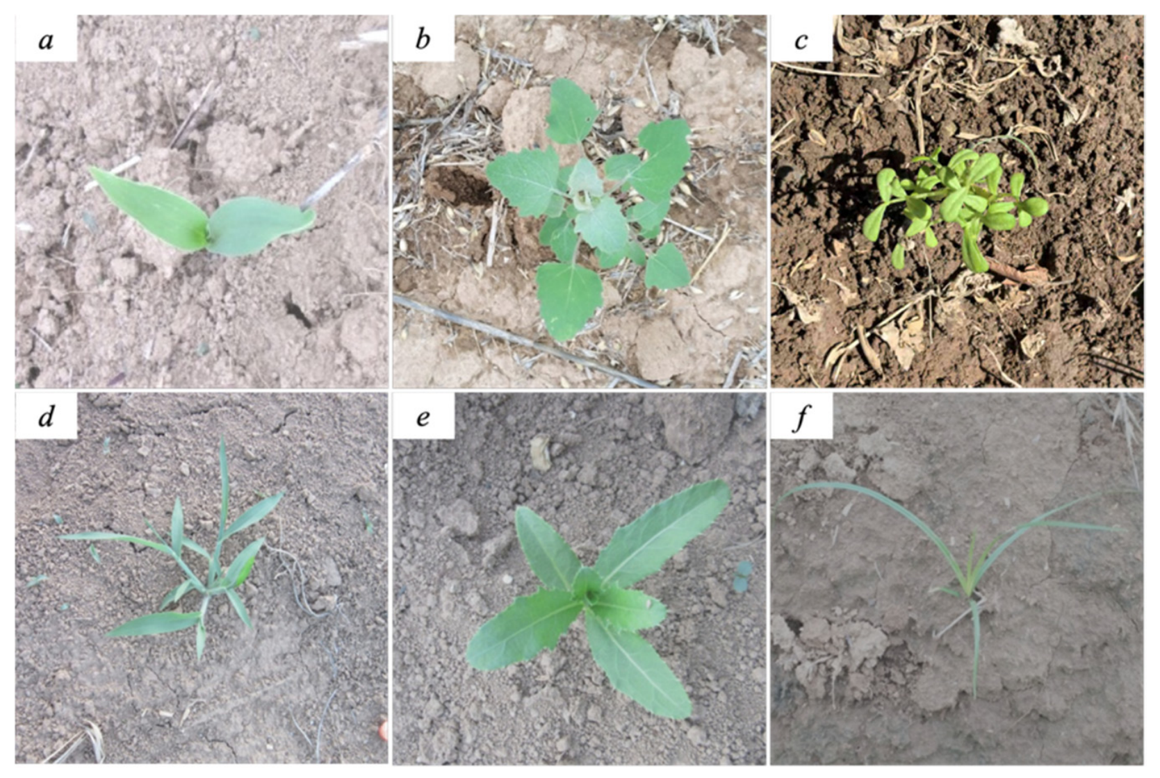
The maize seedling and field weed images used in this study were collected from June to August 2025 under sunny, cloudy, and naturally varying illumination conditions. Images were acquired using an Intel RealSense D435i camera (Intel Corporation, Santa Clara, CA, USA) in the standardized experimental field of Jilin Agricultural University. The image dataset focused on maize seedlings and associated weeds at the seedling stage, comprising 2099 original images. Specifically, the dataset included 367 images of Chenopodium album L., 349 images of Portulaca oleracea L., 366 images of Digitaria sanguinalis L., 361 images of Cirsium arvense var. integrifolium, 324 images of Cyperus rotundus L., and 332 images of maize seedlings. The dataset was divided into training, validation, and test sets at a ratio of 8:1:1, resulting in 1679 training images, 210 validation images, and 210 test images. To improve model adaptability under varying illumination, background conditions, and plant postures, data augmentation was applied only to the training set. The augmentation operations included image blurring, brightness adjustment, shadow addition, horizontal and vertical flipping, and Gaussian noise addition. After augmentation, the training set was expanded to 5037 images. Image annotation was performed using LabelMe (version 1.8.6), and the annotation results were converted into YOLO format for subsequent model training and validation in Figure 1.
Figure 1. Pictures of weeds (a) maize seedling (b) Chenopodium album L. (c) Portulaca oleracea L. (d) Digitaria sanguinalis L. (e) Cirsium arvense var. integrifolium (f) Cyperus rotundus L.
Agronomy 16 01716 g001

2.2. MSDNet

YOLOv8n was selected as the baseline model for maize seedling detection [31]. As a lightweight member of the YOLOv8 series, it offers fewer parameters, lower computational cost, and faster inference, making it suitable for resource-constrained field platforms requiring real-time performance and low deployment cost. However, in complex maize fields, similar colors, spatial overlap, and scale variation between maize seedlings and weeds can reduce detection accuracy and stability.
To address these limitations, YOLOv8n was improved to develop MSDNet, a lightweight maize detection model. A lightweight feature extraction structure and an enhanced feature fusion module were introduced into the backbone to reduce complexity and strengthen seedling feature representation. An attention mechanism was added to emphasize maize seedling regions and spatial information, while Wise-IoU (WIoU) loss was used to improve bounding box regression, convergence stability, and localization accuracy. MSDNet provides a reliable basis for subsequent crop region exclusion and weed stem localization, as shown in Figure 2.

2.2.1. ShuffleNetV2 Network

ShuffleNetV2 is a lightweight convolutional neural network designed for resource constrained devices [32]. Compared with ShuffleNetV1, ShuffleNetV2 emphasizes practical inference speed rather than relying solely on floating point operations as the efficiency metric. Inference efficiency is affected not only by computational cost, but also by channel allocation, the number of group convolutions, branch complexity, and elementwise operations. Therefore, ShuffleNetV2 improves channel splitting, feature fusion, and channel shuffle operations to reduce computational overhead while maintaining strong feature representation, making it suitable for embedded and real time field detection platforms.
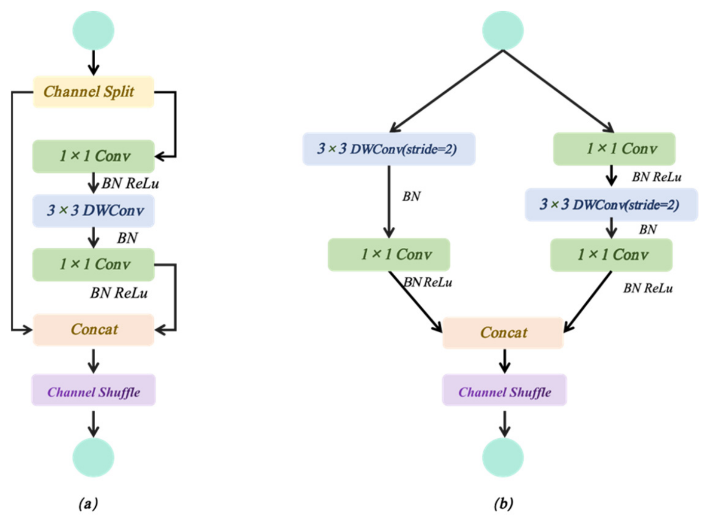
The basic structure of ShuffleNetV2 consists of a feature extraction unit and a downsampling unit, as shown in Figure 3a,b. In the feature extraction unit, the input feature map is split into two branches along the channel dimension. One branch is retained through identity mapping, while the other performs pointwise convolution, depthwise convolution, and pointwise convolution to extract discriminative features. The outputs of the two branches are then concatenated, followed by channel shuffle to enhance information exchange across channels. This design reduces redundant computation and improves feature flow, thereby enhancing model representation and inference efficiency.
The downsampling unit reduces the spatial resolution of feature maps and enlarges the receptive field. Unlike the feature extraction unit, it does not split channels, but extracts features through two parallel branches and concatenates their outputs. This structure preserves effective feature information while increasing network depth and receptive field, enabling the model to capture richer contextual features and improving detection robustness under complex field backgrounds.
Depthwise separable convolution introduced in ShuffleNetV2 can substantially reduce the number of model parameters and computational complexity. Let the height and width of the input feature map be H and W , respectively, the number of input channels be C i n , the number of output channels be C o u t , and the convolution kernel size be K × K . Without considering the bias term, the number of parameters P s t d and the computational cost F s t d of a standard convolution can be expressed as follows:
P s t d = K 2 C i n C o u t
F s t d = H W C i n C o u t K 2
Depthwise separable convolution consists of depthwise convolution and pointwise convolution. Accordingly, its number of parameters P d s and computational cost F d s can be expressed as follows:
P d s = K 2 C i n + C i n C o u t
F d s = H W K 2 C i n + C i n C o u t
As shown by the above equations, compared with standard convolution, depthwise separable convolution can markedly reduce the number of parameters and computational cost while maintaining feature extraction capability. Based on these advantages, ShuffleNetV2 was introduced into the backbone of YOLOv8n to replace part of the original feature extraction structure. This modification reduces model complexity and improves the deployment efficiency and practical adaptability of the model for real time weed detection in maize fields.

2.2.2. C2f-MBSE Network

To improve feature fusion and lightweight representation, the original C2f structure was replaced by C2f-MBSE. C2f promotes gradient flow and feature reuse through cross stage feature splitting and fusion with low computational cost. Since maize seedlings and weeds often exhibit similar morphologies, pronounced scale variation, and complex background interference, MBConv was embedded into C2f to enhance key feature extraction and detection robustness.
MBConv comprises channel expansion, depthwise separable convolution, channel attention recalibration, and channel compression. A 1 × 1 pointwise convolution first expands input channels by a factor of e to improve intermediate feature representation. Depthwise separable convolution then extracts spatial features with lower computation while preserving local texture and edge information. The Squeeze and Excitation (SE) mechanism adaptively recalibrates channel importance to emphasize maize seedling related discriminative features. Finally, another 1 × 1 pointwise convolution compresses the feature maps to the target output channels for dimension recovery and information integration. As shown in Figure 4, C2f-MBSE improves feature representation and detection stability, supporting subsequent crop region exclusion and weed stem localization.

2.2.3. CA Mechanism

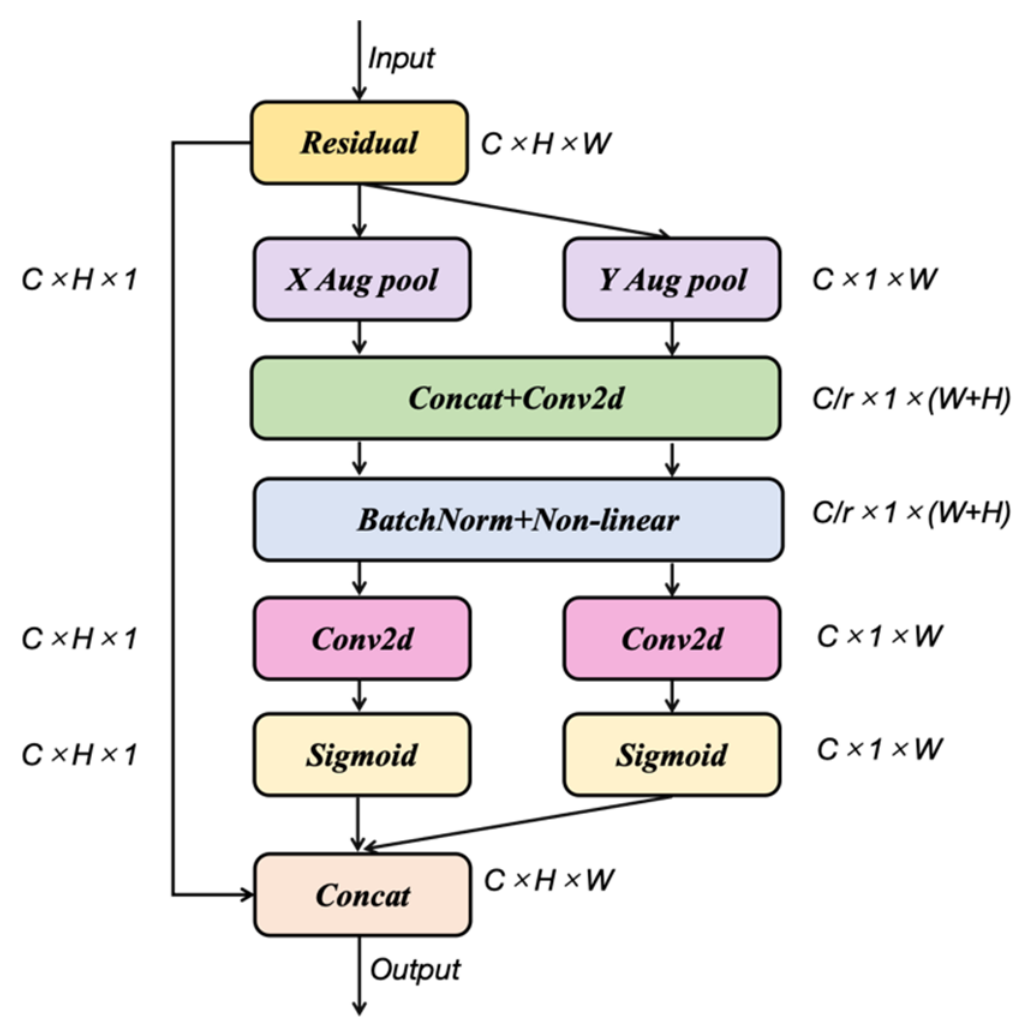
To reduce model complexity, ShuffleNetV2 was used to replace part of the original feature extraction structure in the YOLOv8n backbone. However, although this lightweight modification reduces the number of parameters and computational cost, it may weaken the network’s ability to represent fine grained maize seedling features, thereby affecting detection accuracy. To address this issue, the Coordinate Attention (CA) mechanism was embedded at the end of the ShuffleNetV2 backbone to enhance feature representation and spatial localization capability, as shown in Figure 5.
The CA module is a lightweight attention unit that jointly models channel dependencies and spatial position information. For an intermediate input feature tensor X = [ x 1 , x 2 , , x C ] R C × H × W , where C , H , and W denote the number of channels, feature map height, and feature map width, respectively, the CA module encodes spatial information separately along the horizontal and vertical directions. In this way, positional information is embedded into the channel attention modeling process, generating an output feature tensor Y = [ y 1 , y 2 , , y C ] with the same size as the input. This mechanism enables the network to emphasize informative channel responses while preserving the direction and location information of target regions, thereby improving its perception of maize seedling leaf edges, morphological structures, and spatial distribution. Owing to its low computational overhead, the CA module can improve detection accuracy and robustness in complex field backgrounds while maintaining deployment efficiency, providing more reliable detection results for subsequent crop region exclusion and weed stem localization.

2.2.4. W I o U Loss Function

In object detection, the bounding box regression loss directly affects localization accuracy. The C I o U loss considers the overlap area, center point distance, and aspect ratio consistency between the predicted and ground truth boxes, thereby improving bounding box regression to some extent. In this formulation, L I o U   denotes the intersection over union loss between the predicted and ground truth boxes, α   is a weighting function used to balance different constraint terms, and v measures aspect ratio consistency. However, when the aspect ratios of the predicted and ground truth boxes are linearly correlated, the aspect ratio penalty term in C I o U may become ineffective, resulting in limited gradient guidance during regression. In addition, both overly high quality and low quality regression samples may affect bounding box optimization, thereby restricting further improvement in localization performance.
To address these limitations, this study adopts the W I o U loss to replace the original bounding box regression loss. W I o U dynamically assigns gradient gains according to the quality of regression samples, reducing the adverse gradients generated by low quality samples while preventing high quality samples from dominating the optimization process. As a result, the model can focus more effectively on bounding box regression optimization. The W I o U loss is defined as follows:
L W I o U = r R W I o U L I o U , R W I o U 1 , e , L I o U 0,1
where R W I o U denotes the distance attention mechanism, which enhances the influence of the center distance between the predicted box and the ground truth box on the regression loss. The term r represents the non monotonic focusing coefficient, which dynamically adjusts the gradient gain according to sample quality. R W I o U and r are defined as follows:
R W I o U = exp ( x x g t ) 2 + ( y y g t ) 2 ( W g 2 H g 2 )
r = β δ α β δ
where x y and x g t y g t denote the center coordinates of the predicted box and the ground truth box, respectively. W g and H g represent the width and height of the minimum enclosing rectangle covering both the predicted and ground truth boxes, respectively. The symbol indicates that this term does not participate in gradient update during backpropagation. The outlier degree factor β is defined as follows:
β = L I o U L I o U
where L I o U denotes the I o U loss of the current regression sample, L I o U represents the dynamic moving average of the I o U loss, and α and δ are hyperparameters. By introducing the outlier degree factor, W I o U adaptively adjusts the loss weight according to the regression quality of each sample. For high quality samples, the model can already achieve accurate localization, and assigning excessive gradient gain provides limited additional benefit. In contrast, low quality samples often contain more noise or localization deviation, and excessive optimization may introduce harmful gradients. Therefore, W I o U reduces the gradient gains of both high quality and low quality samples and shifts the training focus toward ordinary quality samples, thereby improving the stability and effectiveness of bounding box regression.
Compared with C I o U , W I o U removes the aspect ratio penalty term, avoiding the potential failure of aspect ratio constraints under specific conditions. Moreover, its dynamic non monotonic focusing mechanism more effectively balances the influence of regression samples with different qualities during model training, which helps improve target localization and generalization performance under complex field backgrounds. Therefore, this study adopts the W I o U loss function to replace the original bounding box regression loss, thereby enhancing the localization accuracy and training robustness of the maize seedling detection model.

2.3. Crop Area Exclusion and Weed Area Segmentation

The objective of this study was to extract all weed regions in the field after excluding interference from maize seedlings, thereby providing a reliable image basis for subsequent weed stem localization. If green vegetation regions are directly extracted from original field images, both maize seedlings and weeds are identified as targets, which may cause crop region misclassification and affect subsequent weed contour analysis and stem center estimation. Therefore, crop regions were first masked according to the maize seedling detection results, and the pixels corresponding to maize seedlings were set to zero to achieve crop region exclusion. Green vegetation segmentation and soil background suppression were then performed on the crop excluded images.
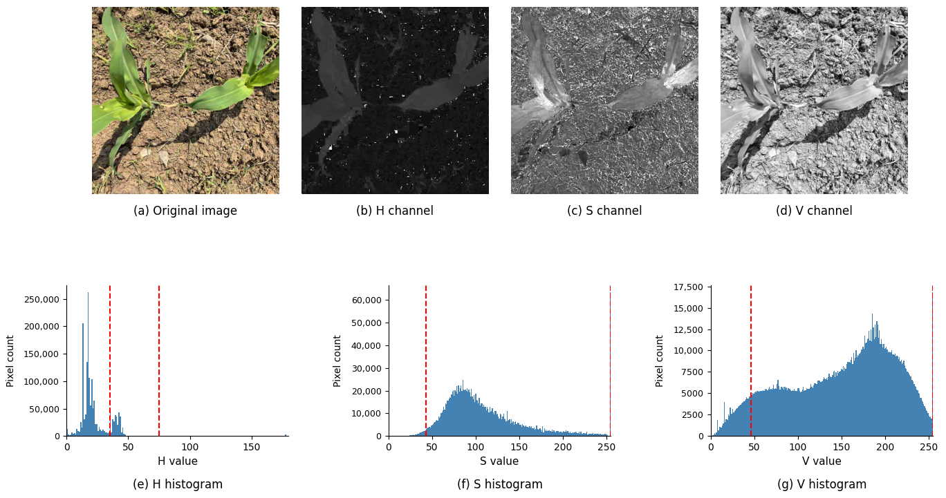
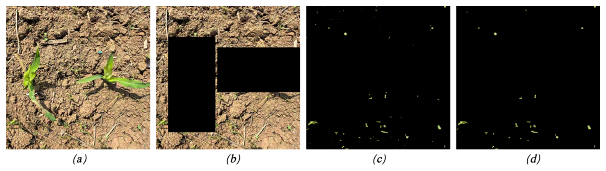
In the HSV color space, soil and green vegetation show distinct differences in hue, saturation, and value distributions, allowing color thresholding to be used for image segmentation after crop exclusion. In this study, the pixels corresponding to the detected maize seedling regions in Figure 6a were set to zero, producing the crop excluded image shown in Figure 6b. The processed RGB image was then converted into the HSV color space. Based on the color distribution of green vegetation in field images, the threshold ranges were set to [35, 55] for the H channel, [43, 255] for the S channel, and [46, 255] for the V channel. The cv2.inRange function was used to generate a binary mask of green vegetation, thereby preliminarily separating weed regions from the soil background. An AND operation was then applied between the vegetation mask and the original image to obtain the preliminary segmentation result shown in Figure 6c.
Because field images often contain interference from uneven illumination, soil particles, shadows, and small vegetation fragments, the preliminary segmentation result may include noise points and holes. To further improve the completeness and accuracy of weed region extraction, morphological processing was applied to optimize the binary mask. Erosion was first used to remove small scale noise and isolated false targets, followed by dilation to fill small holes within weed regions and restore target contours. Finally, the morphologically processed mask was combined with the crop excluded image using another AND operation, producing the weed region extraction result shown in Figure 6d. This processing pipeline effectively suppresses soil background interference and preserves green weed vegetation regions after maize seedling exclusion, providing input for subsequent weed stem localization based on contour analysis, principal component analysis, and image moments.

2.4. PCA Algorithm

To accurately localize weed stems after crop-region exclusion, this study combined HSV-based segmentation with principal component analysis (PCA) to estimate the principal-axis direction of weed contours. After maize region masking, HSV color filtering, and morphological processing, the remaining green vegetation regions in the image were regarded as weed targets. Because weed leaves often have irregular shapes and markedly different contour orientations, directly using the centroid of the weed region as the stem center may lead to localization errors caused by asymmetric leaf distribution. Therefore, PCA was first used to extract the main extension direction of the weed contour point set, and image moments were then used to calculate the centroid of the weed region. The centroid was further projected onto the principal axis to estimate the weed stem center.
The purpose of PCA is to identify the direction with the maximum variance in the data distribution and use it as the principal axis of the target contour. For weed contours, the spatial distribution of contour points in the image plane reflects the main morphological characteristics of the weed region. By constructing the covariance matrix of contour point coordinates and performing eigenvalue decomposition, the eigenvector representing the dominant extension direction of the weed can be obtained, providing a geometric basis for subsequent stem center estimation.
The specific procedure is as follows. Suppose that a weed contour consists of N pixels, and its point set is expressed as:
P = p 1 , p 2 , , p N
where the coordinates of the i -th contour point are given by:
p i = ( x i , y i ) T
First, the mean vector of the contour point set is calculated as follows:
μ = 1 N i = 1 N p i
Then, the centered coordinate of each contour point relative to the mean vector is computed as:
ϕ i = p i μ
The covariance matrix of the contour point set is then constructed as follows:
C = 1 N i = 1 N ϕ i ϕ i T
where C represents the covariance matrix of the two-dimensional contour point set. The eigenvalue decomposition of C is expressed as:
C v j = λ j v j
where λ j denotes the j   eigenvalue, and v j is its corresponding eigenvector. The eigenvector associated with the largest eigenvalue represents the direction of maximum variance in the contour point set, which is defined as the principal axis direction of the weed contour.
v m a x = v j , λ j = max λ 1 , λ 2
After obtaining the principal axis direction of the weed, image moments were further used to calculate the centroid of the weed region. Let the binary image of the weed region be I ( x , y ) , where weed pixels are assigned a value of 1 and background pixels are assigned a value of 0. The spatial moments are then defined as follows:
M p q = x y x p y q I x , y
The centroid of the weed region is then given by:
c = ( x c , y c ) T = M 10 M 00 M 01 M 00 T
where M 00 denotes the area of the weed region, M 10 and M 01 denote the first order spatial moments, and c = ( x c , y c ) T represents the centroid coordinates of the weed region. Considering that the uneven distribution of weed leaves may cause the centroid to deviate from the actual stem position, the centroid c calculated from image moments was projected onto the principal axis extracted by PCA, and the resulting projection point was used as the estimated weed stem center. Let the principal axis pass through the mean point μ of the contour point set, with v m a x as its direction vector. The projection point s of the centroid c on the principal axis can be expressed as Equation (18), where s denotes the estimated position of the weed stem center.
s = μ + c μ T v m a x v m a x
This method geometrically corrects the centroid position by exploiting the overall spatial distribution of the weed contour, thereby reducing the influence of irregular leaf morphology, variations in target posture, and local contour deviation on stem localization. It does not rely on multiclass weed recognition or fine grained category annotation, and can achieve geometric localization of weed stems under complex maize seedling field backgrounds, providing target-location information for subsequent site-specific weed-control operations.

2.5. Weed Stem Localization Based on Crop Region Exclusion

In maize seedling fields, weeds vary greatly in species, morphology, scale, leaf structure, and growth posture. Accurate recognition of multiple weed categories usually requires large scale datasets covering different species, growth stages, and density levels, together with extensive precise annotation. In addition, weed samples differ markedly across regions, which limits the generalization of conventional recognition models and makes stable detection difficult even within the same crop field environment. High-precision localization of weed stems is therefore an important prerequisite for precision weed control.
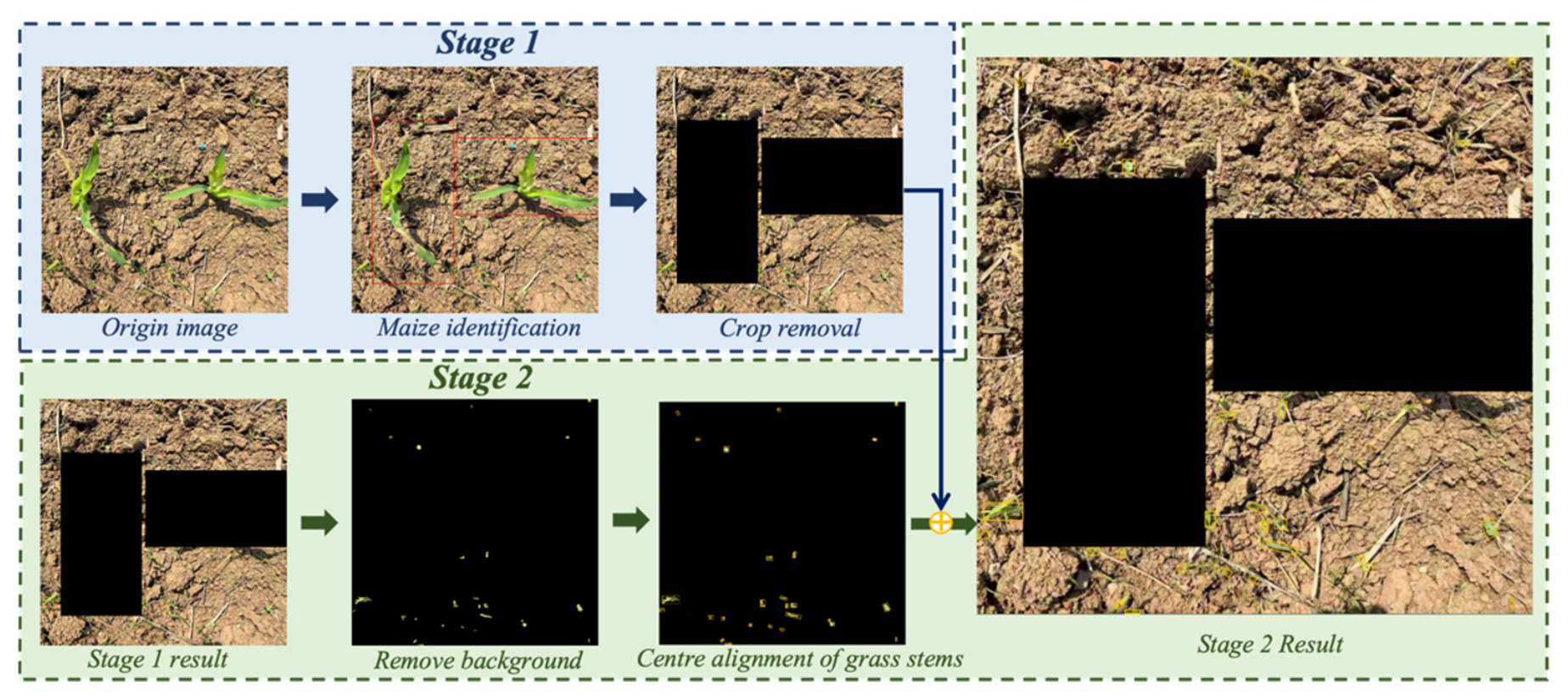
To address these issues, this study proposes a two-stage weed stem localization method based on crop region exclusion. Instead of identifying weed categories individually, the method first detects and removes maize seedling regions, then extracts the remaining green vegetation and estimates weed stem centers using contour geometric features. The overall workflow is shown in Figure 7.
In the first stage, the improved detection model identifies maize seedlings and obtains their bounding boxes. Pixels within the detected maize seedling boxes are set to zero to mask crop regions, reducing crop interference during subsequent vegetation segmentation and preventing maize seedlings from being misclassified as weeds.
In the second stage, HSV color filtering is applied to the crop excluded image to extract green vegetation. Morphological processing and area thresholding are then used to remove soil noise, shadows, and small false targets, yielding complete weed candidate contours. PCA is performed on each weed contour to extract the principal axis direction, while image moments are used to calculate the weed centroid. The centroid is projected onto the PCA derived principal axis, and the projection point is taken as the estimated weed stem center. The minAreaRect function is also used to describe the spatial posture of weed contours.
Finally, the estimated stem centers are overlaid on the processed images for visual verification. This method avoids multiclass weed modeling, reduces annotation requirements, and provides target-location information for precision weeding in complex maize seedling fields.

2.6. Evaluation Metric Settings

Precision (P), recall (R), mean average precision (mAP), model size, and detection speed were used as evaluation metrics in this study. The corresponding calculation formulas for selected metrics are given as follows:
P = T P T P + F P
R = T P T P + F N
A P = 0 1 P r d r  
m A P = 1 C i = 1 c A P i
where T P denotes the number of positive samples correctly predicted as positive, F P denotes the number of negative samples incorrectly detected as positive, and F N denotes the number of positive samples that are not detected. C represents the number of classes. In addition, i , f , and ο denote the input size, convolution kernel size, and output size, respectively.
Since all weeds were treated as a single target category during the weed detection stage, the background segmentation algorithm was evaluated using mean pixel accuracy (MPA). Its calculation formula is defined as follows:
P A = T P + T N T P + T N + F T + F N
M P A = 0 N P A i N
where N denotes the total number of samples in the dataset, and P A i represents the pixel accuracy of the i -th image.
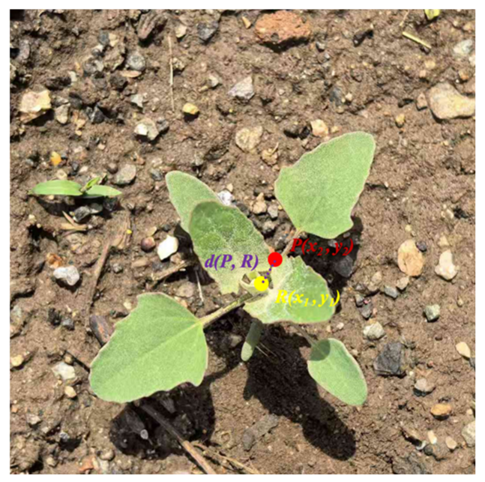
To evaluate the localization accuracy of weed stem centers, the stem center points predicted by the algorithm were matched with manually annotated ground truth stem centers. Let the predicted point be P ( x 2 , y 2 ) and the ground truth point be R ( x 1 , y 1 ) . The Euclidean distance between them is defined as d ( P , R ) = x 2 x 1 ) 2 + ( y 2 y 1 ) 2 , as shown in Figure 8. Here, d ( P , R ) represents the pixel distance between the predicted and ground truth stem center points. A smaller distance indicates that the localization result is closer to the manual annotation. In this study, a distance threshold d thresh was defined. When the distance between a predicted point and a ground truth point satisfied d ( P , R ) d thresh , the prediction was considered correct and counted as a TP. If a ground truth stem center was not successfully matched by any predicted point, it was counted as an FN. If a predicted point failed to match any ground truth point, it was counted as a FP. To prevent multiple predicted points from being assigned to the same ground truth point, a one to one nearest neighbor matching strategy was adopted during the matching process.
Based on the above statistical results, precision P , detection rate D , and miss detection rate M were used to evaluate the weed stem center detection performance. These metrics are calculated as follows:
P = T P T P + F P
D = T P T P + F N
M = 1 D = F N T P + F N
where P r denotes the proportion of predicted stem center points that are correctly localized, D represents the proportion of ground truth weed stem centers that are successfully detected, and M indicates the proportion of ground truth weed stem centers that are missed. To further evaluate the localization error of stem centers, the mean Euclidean distance between successfully matched point pairs was calculated as follows:
M E D = 1 K i = 1 K d i
To further quantify the pixel-level localization error of weed stem centers, RMSE and MAE were calculated based on the Euclidean distance d ( P i , R i ) between each successfully matched predicted stem center and its corresponding manually annotated ground-truth stem center, as defined above and illustrated in Figure 8. RMSE and MAE are defined as follows:
R M S E = 1 K i = 1 K [ d ( P i , R i ) ] 2
M A E = 1 K i = 1 K d ( P i , R i )
where K denotes the number of successfully matched weed stem center pairs, P i denotes the predicted stem center of the i -th matched pair, R i denotes the corresponding manually annotated ground-truth stem center, and d ( P i , R i )   denotes the Euclidean distance between P i and R i . The value of d P i , R i measured in pixels. Smaller RMSE and MAE values indicate lower pixel-level localization errors. These two metrics evaluate localization error rather than image-level counting error.
To evaluate whether the predicted stem center was sufficiently close to the manually annotated reference point, a pixel-distance tolerance criterion was adopted. Based on the camera calibration results and image spatial resolution, d thresh was set to 15 pixels, corresponding to an actual spatial deviation of approximately 9.5 mm. A prediction was considered correct when the distance between the predicted stem center and the manually annotated reference point did not exceed this threshold. This criterion provides a direct and quantitative measure of weed stem localization accuracy for precision weeding.

3. Results and Analysis

3.1. Experimental Design

The training process used the Adam optimizer with a learning rate of 0.001. Both models were trained for 200 epochs with a batch size of 12. Model training was conducted on a high performance server equipped with an Intel® Core™ i7 14700KF processor, 64 GB of RAM, and an NVIDIA GeForce RTX 4090D GPU with 24 GB of video memory. The software environment consisted of Ubuntu 20.04, PyCharm 2023, Python 3.10, and the PyTorch 2.1.2 deep learning framework.
To evaluate the performance of the model in resource constrained environments, deployment and testing were also conducted on an NVIDIA Jetson TX2 edge computing device. The Jetson TX2 integrates a 256 core Pascal GPU and an ARM Cortex A57 CPU, with 8 GB of LPDDR4 memory and a typical power consumption ranging from 7.5 W to 15 W. The software environment on the edge device consisted of Ubuntu 20.04.5 LTS, Python 3.8, and PyTorch 1.8.0.

3.2. Ablation Experiment

To evaluate the contribution of each improved module to maize seedling detection performance, ablation experiments were conducted using YOLOv8n as the baseline model. ShuffleNetV2, C2f-MBSE, the CA mechanism, and the W I o U loss function were introduced separately, and the experimental results are presented in Table 1.
As shown in Table 1, the original YOLOv8n achieved an mAP@0.5 of 84.7%, with a model size of 6.3 MB and 3.21 M parameters. After replacing the backbone with ShuffleNetV2, Model-1 reduced the model size to 4.9 MB and the parameters to 2.35 M, while increasing mAP@0.5 to 86.5%, indicating that ShuffleNetV2 reduced model complexity without impairing detection performance.
Introducing C2f-MBSE alone increased the mAP@0.5 of Model 2 to 89.9%, 5.2 percentage points higher than the baseline. Adding the CA mechanism alone further improved the mAP@0.5 of Model 3 to 91.4%. These results indicate that C2f-MBSE enhances feature fusion and local feature extraction, whereas CA helps the model focus on key maize seedling regions and reduces background interference.
The combined experiments show that the modules are complementary. Model-4, which integrated ShuffleNetV2 and C2f-MBSE, further reduced model size and parameters, but its mAP@0.5 was lower than that of Model-2, suggesting that the lightweight backbone may weaken part of the deep semantic information while reducing redundant computation. After adding CA, Model-7 achieved mAP@0.5, Precision, and Recall of 92.6%, 94.9%, and 93.2%, respectively, indicating that CA partly compensates for the limited feature representation of the lightweight network. Based on Model-7, MSDNet further introduced W I o U loss, increasing mAP@0.5 and Recall to 93.4% and 93.7%, respectively. Although Precision decreased slightly, overall detection accuracy and recall improved, confirming the positive effect of W I o U on bounding box regression.
Compared with YOLOv8n, MSDNet improved mAP@0.5 by 8.7 percentage points, Precision by 4.2 percentage points, and Recall by 5.9 percentage points, while reducing model size from 6.3 MB to 4.8 MB and parameters from 3.21 M to 2.29 M. These results demonstrate that MSDNet improves maize seedling detection accuracy while reducing model complexity.
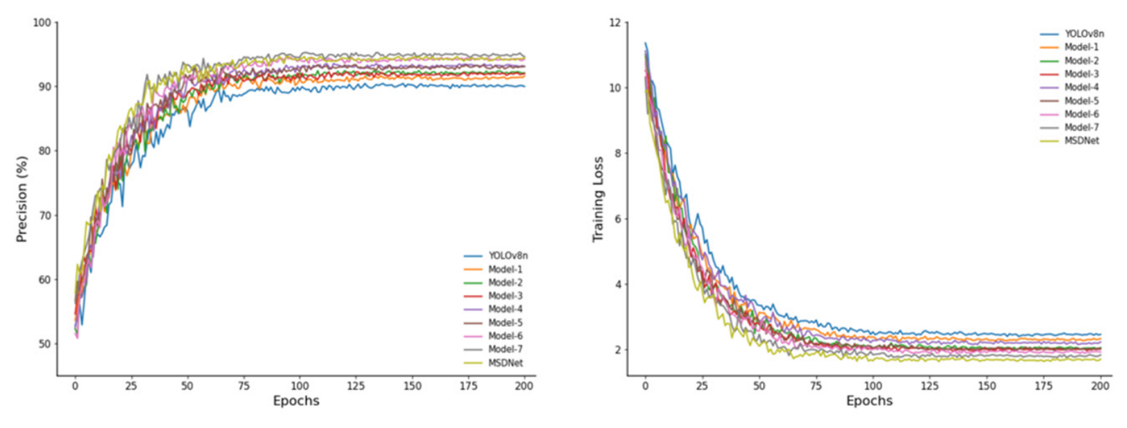
Figure 9 shows the training loss and accuracy trends of different models. Compared with the baseline YOLOv8n, the improved models achieved faster convergence, lower final loss, and higher detection accuracy, indicating that the introduced modules enhanced both training stability and detection performance. Among them, MSDNet maintained a low and stable loss after convergence, while its accuracy remained at a high level. This demonstrates that the integration of ShuffleNetV2, C2f-MBSE, the CA mechanism, and W I o U loss improves feature extraction, feature fusion, and bounding box regression. Overall, MSDNet improves maize seedling detection accuracy while maintaining a lightweight structure, achieving a favorable balance between detection performance and model complexity. Therefore, it is more suitable for maize recognition tasks under complex field conditions.

3.3. Comparative Experiments on Lightweight Networks

To select a lightweight backbone network suitable for maize detection, EfficientNet- Lite, GhostNet, MobileNetV2, MobileNetV3, and ShuffleNetV2 were separately introduced into the YOLOv8n framework to replace the original backbone. Comparative experiments were conducted under the same training parameters and testing environment. The experimental results are presented in Table 2.
As shown in Table 2, different lightweight backbone networks had varying effects on detection performance and model complexity. Compared with the original YOLOv8n, EfficientNet Lite, MobileNetV3, and ShuffleNetV2 improved mAP@0.5 to different extents. Among them, ShuffleNetV2 achieved the largest improvement, reaching an mAP@0.5 of 86.5%, which was 1.8 percentage points higher than the baseline. Its Precision and Recall reached 91.3% and 89.1%, respectively, both exceeding those of the original YOLOv8n. This indicates that ShuffleNetV2 can better preserve effective feature representations of maize seedlings under complex field backgrounds.
In terms of model complexity, all lightweight backbones reduced both model size and parameter number. ShuffleNetV2 achieved a model size of only 4.9 MB and 2.35 M parameters, representing reductions of 22.2% and 26.8%, respectively, compared with the original YOLOv8n. This demonstrates its strong lightweight performance among the tested networks. Although GhostNet and MobileNetV3 also reduced model complexity, their mAP@0.5 and Recall were lower than those of ShuffleNetV2. EfficientNet-Lite improved mAP@0.5, but its lower Precision suggests relatively limited suppression of complex background interference in this task. Overall, ShuffleNetV2 achieved the best comprehensive detection performance while maintaining a lightweight structure. Therefore, ShuffleNetV2 was selected as the lightweight backbone of YOLOv8n to support subsequent model improvements.

3.4. Comparison of Segmentation Algorithms

Accurate separation of green vegetation from the soil background is fundamental to maize seedling region extraction and weed stem localization. Based on the distribution differences between vegetation and soil in the HSV color space in maize seedling field images, the threshold ranges were set to H [35, 55], S [43, 255], and V [46, 255] to extract green vegetation regions.
Among the three channels, the H channel was used as the primary discriminative feature to distinguish green vegetation from the soil background, while the S and V channels served as auxiliary constraints to suppress low saturation regions, shadows, and dark background interference. As shown in Figure 10, green vegetation pixels were mainly concentrated within the specified H channel range. By combining this range with the S and V channel constraints, the stability of vegetation segmentation under complex field conditions was effectively improved, providing a reliable basis for subsequent maize seedling exclusion and weed stem center localization.
To verify the effectiveness of the green vegetation segmentation method used in this study, 100 images were randomly selected and manually annotated to generate segmentation mask images for performance evaluation. Comparative experiments were conducted using three methods: G channel combined with Otsu thresholding, H channel combined with Otsu thresholding, and HSV threshold segmentation combined with morphological processing. The results are presented in Table 3.
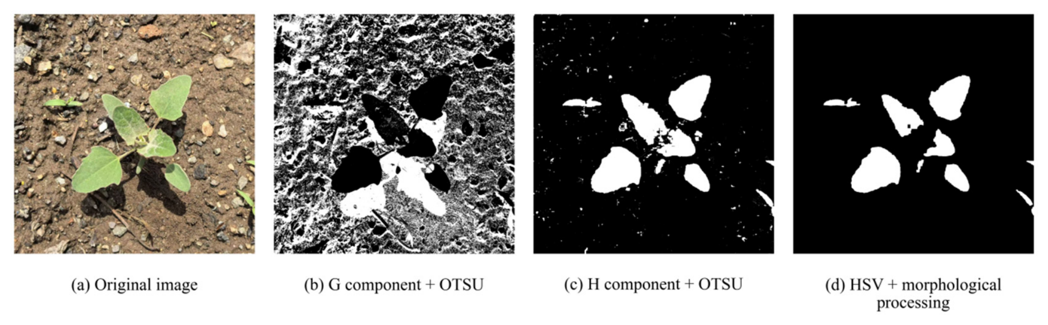
As shown in Table 3, the G channel combined with Otsu thresholding was sensitive to soil color, shadows, and illumination variation, achieving an MPA of 84.6% and an mIoU of 76.6%, with frequent background misclassification. The H channel combined with Otsu thresholding improved segmentation by using hue information, reaching an MPA of 89.7% and an mIoU of 82.4%. In contrast, HSV threshold segmentation combined with morphological processing achieved the best performance, with an MPA of 97.6% and an mIoU of 93.8%, indicating that it extracted green vegetation more completely while effectively suppressing soil background noise. Although its average processing time was 0.08 s, slightly higher than those of the other methods, it still satisfied the real time requirements for subsequent maize seedling extraction and weed stem localization.
Figure 11 shows the segmentation results on randomly selected maize seedling field images. The G channel Otsu and H channel Otsu methods extracted only part of the vegetation and still produced noise, background misclassification, and discontinuous vegetation regions, which could affect subsequent maize seedling exclusion and weed stem localization. By contrast, the HSV thresholding and morphological processing method reduced soil noise and produced more complete and continuous vegetation regions. Therefore, this study adopted combined H, S, and V channel thresholding with morphological processing for soil background segmentation and green vegetation extraction.
To evaluate the robustness of H-channel threshold selection, a sensitivity analysis was conducted on 100 manually annotated test images. Specifically, while keeping the S and V thresholds unchanged, the original H-channel threshold range of H [35, 55] was moderately expanded and narrowed. MPA, mIoU, and the green area ratio were used to evaluate the influence of threshold variation on segmentation performance, as shown in Table 4. The original threshold setting of H [35, 55], S [43, 255], and V [46, 255] achieved the best overall segmentation performance. When the H range was slightly expanded to [32, 58] or narrowed to [38, 52], the MPA and mIoU decreased only slightly, indicating that moderate changes in the H-channel threshold range did not cause obvious degradation in segmentation performance. When the H range was further expanded to [30, 60], the green area ratio increased to 18.9%, suggesting that more green regions were extracted, but some soil or shadow noise may also have been introduced. In contrast, when the H range was narrowed to [40, 50], the green area ratio decreased to 15.8%, and the mIoU dropped to 91.9%, indicating that an overly narrow H range may omit some light-green vegetation regions. Overall, under the sampled maize seedling field conditions, the selected HSV thresholds showed a certain degree of tolerance to moderate threshold variation and provided relatively stable green vegetation regions for subsequent weed stem localization.

3.5. Weed Stem Positioning Experiment

To evaluate the weed stem localization performance of the proposed method under maize seedling field conditions, the remaining green vegetation was segmented and used for stem center localization after maize seedling detection and crop region exclusion. MSDNet was first used to detect maize seedlings, and the crop regions within the detected bounding boxes were masked to reduce their interference with weed extraction. Then, HSV threshold segmentation and morphological processing were applied to extract the remaining green vegetation. Weed stem centers were estimated using contour features, image moments, and PCA based principal axis analysis.
The Euclidean distance between the predicted stem center and the manually annotated ground truth was used to evaluate localization accuracy. A localization result was considered correct when the pixel distance was less than or equal to the predefined threshold. To relate the pixel threshold to the actual physical deviation, a geometric derivation between pixel-based localization error and spatial distance was conducted. Before calculating the localization error, the ground-truth weed stem centers were manually annotated on the original field images. For each visible weed instance, the ground-truth point R ( x 1 , y 1 ) was defined as the visible stem base or growing center, namely the point where the main weed stem or leaf cluster emerged from the soil surface. For partially occluded weeds, if the stem base or growing center was still partially visible, the reference point was placed at the estimated center of the visible stem base according to the remaining vegetation contour and the growth direction of the weed. For severely occluded weeds, if the stem base or growing center was completely hidden and could not be reliably inferred from the image, the sample was regarded as a failure case for precise stem-center localization rather than being assigned an arbitrary ground-truth point. The final ground-truth points were not obtained by averaging multiple independent annotations. The image resolution was 640 × 640 pixels. The camera sensor diagonal was 3.08 mm, and the image aspect ratio was 1:1. Although no inter-annotator agreement index was calculated, the use of a single unified annotation protocol ensured that all reference points were defined and evaluated consistently within the current dataset. Therefore, the effective sensor width W s e n s o r and height H s e n s o r   can be estimated as follows:
W s e n s o r = H s e n s o r = 3.08 2 2.18   mm
Given that the camera focal length f is 1.88 mm, the horizontal field of view (FOV) can be expressed as:
F O V = 2   arctan 2.18 2 × 1.88 60.2
The physical size of a single pixel in the horizontal direction, P w , can be estimated as:
P w = W s e n s o r I m a g e   w i d t h = 2.18 640 0.00341   mm = 3.41   μ m
Therefore, the actual physical length on the sensor corresponding to 15 pixels in the image is:
l = 15 × 0.00341 = 0.0511   mm
Based on the pinhole camera model and the principle of similar triangles, when the imaging distance D is 350 mm, the actual spatial length S corresponding to this sensor length can be expressed as:
S = 350 × 0.0511 1.88 = 9.50   mm
This result indicates that, under the image acquisition conditions used in this study, a localization error of 15 pixels corresponds to an actual spatial deviation of 9.50 mm. Therefore, the 15 pixels threshold adopted in this study can be used as the allowable error range for weed stem localization in maize seedling fields and to evaluate the spatial deviation between the predicted stem center and the manually annotated center.
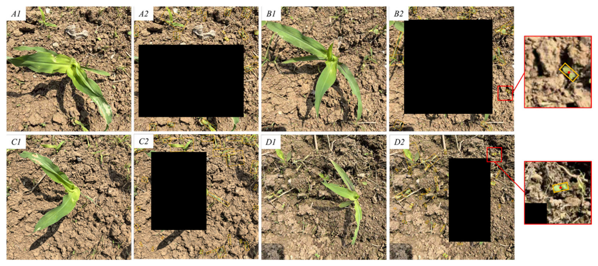
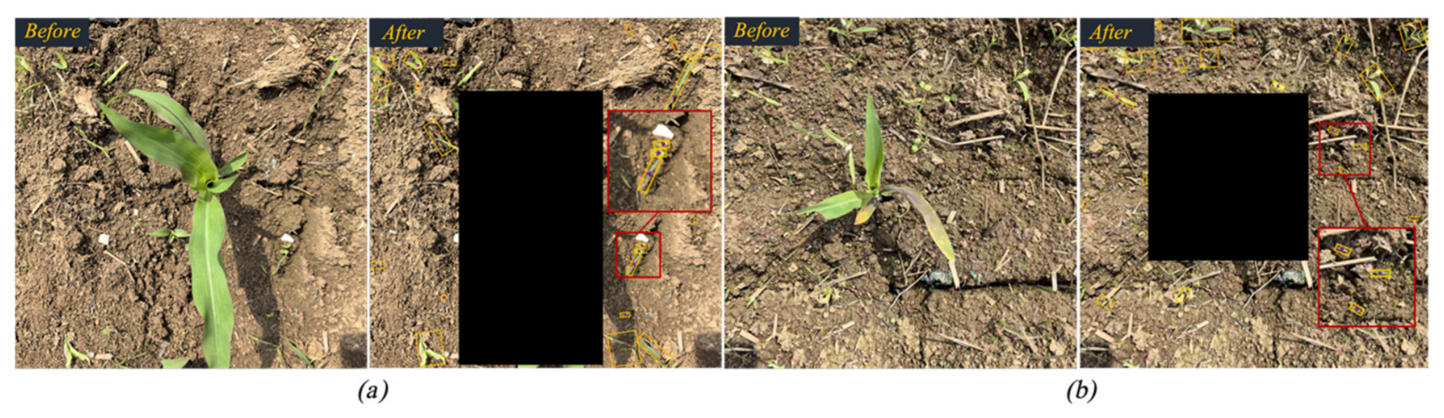
Figure 12 shows the weed stem localization results obtained by the proposed method under different field conditions, including dense weed distribution, sparse weed distribution, strong illumination, and complex soil backgrounds. After maize seedling region exclusion, the proposed method effectively preserved green weed regions and localized their stem centers. For weed targets with relatively complete morphology and limited occlusion, the predicted stem positions were close to the manually annotated locations. However, when weed leaves overlapped, soil background interference was strong, or weeds were located close to maize seedlings, some predicted points showed certain localization deviations.
The weed stem localization results are summarized in Table 5, which reports the actual number of weeds, the number of successfully localized stem centers, and the number of missed detections in each test image. Based on the predefined stem localization threshold, the four test images achieved an average miss detection rate of 9.65% and an average localization accuracy of 90.35%.
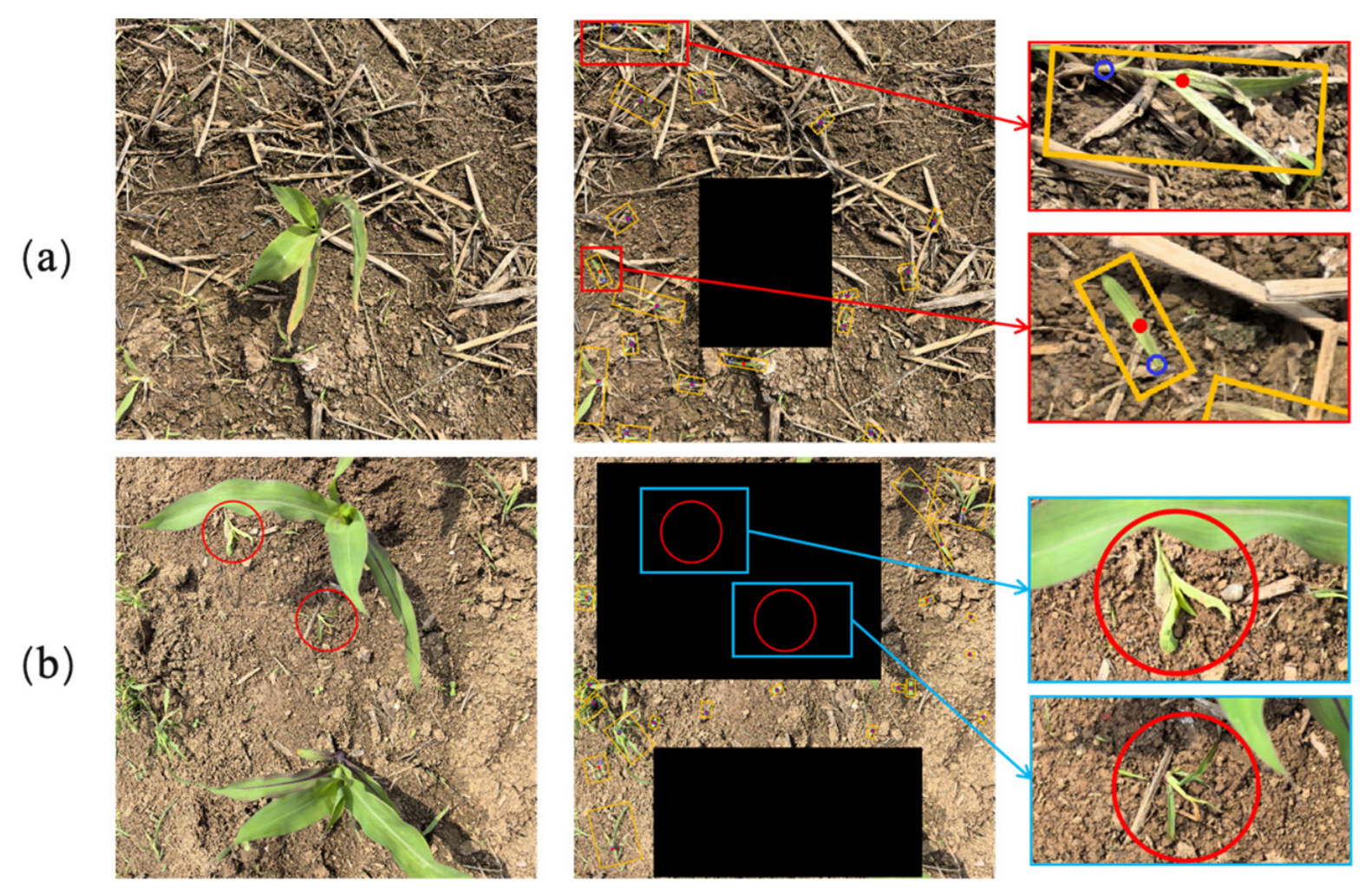
Figure 13 shows the weed stem localization results obtained using the proposed method. The blue circles indicate the weed growing point regions, while the red dots represent the weed stem center positions predicted by the proposed method.
Table 6 presents the weed stem localization results. As shown in the table, the proposed method maintained stable localization performance as the number of test samples increased from 72 to 511. The prediction precision P ranged from 91.4% to 93.7%, with an average of 92.5%; the detection rate D ranged from 88.9% to 91.1%, with an average of 90.1%; and the miss detection rate M was controlled between 8.9% and 11.1%, with an average of 9.9%. In terms of localization error, the mean Euclidean distance of each group ranged from 9.1 to 11.8 pixels, all below the error threshold of 15 pixels, indicating strong consistency between the predicted stem centers and the manually annotated centers. The overall RMSE and MAE were 12.02 pixels and 10.65 pixels, respectively, suggesting that the pixel level localization error of the proposed method remained within an acceptable range. Overall, the proposed method achieved stable weed stem center localization across different sample sizes and can provide reliable positional information for subsequent precision-weeding operations.
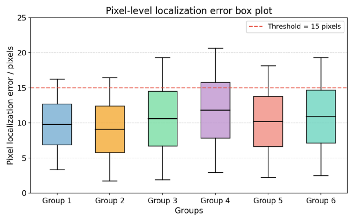
As shown in Figure 14, the pixel level localization error distributions of different test groups were generally stable, with the red dashed line indicating the 15 pixel error threshold. The median localization errors of all groups were below 15 pixels, indicating that most predicted stem centers deviated from the manually annotated ground truth points within the predefined tolerance range. Among them, Group 2 showed relatively smaller localization errors, with a lower box position overall, suggesting better localization accuracy. In contrast, Group 4 exhibited a higher box and upper whisker, indicating increased localization errors for some weed stems. This may be related to complex field backgrounds, overlap between weeds and maize seedlings, or irregular weed morphology. Overall, the RMSE and MAE of the proposed method were 12.02 pixels and 10.65 pixels, respectively, demonstrating that the method achieved stable weed stem localization under maize seedling field conditions and showed good robustness and practical application potential.
Although the proposed weed stem localization method achieved satisfactory localization performance in maize seedling field images, several limitations remain under complex field conditions. As shown in Figure 15a, when weed leaves exhibit irregular morphology, incomplete contours, or skewed growth orientations, the principal axis extracted by PCA may deviate from the actual stem direction. This can cause offsets between the predicted stem centers and the manually annotated ground truth points. Although such cases do not necessarily lead to complete localization failure, they reduce the accuracy of stem center localization and result in local positional deviations.
In addition, although the experiments were conducted in maize seedling fields, the proposed framework does not rely on maize-specific handcrafted rules. Instead, it adopts a modular detection–exclusion–localization pipeline. In this framework, the YOLO-based detector serves as a flexible learning module for crop detection, while crop-dependent visual characteristics can be accommodated through data-driven training or fine-tuning. The subsequent weed stem localization relies on vegetation contours and generic geometric cues rather than explicit weed-species-specific morphological assumptions. Therefore, the proposed framework has the potential to be extended to other row-crop scenarios without changing the core algorithmic structure. However, such extension would still require crop-specific image collection, detector retraining or fine-tuning, and further validation under the corresponding crop morphology, canopy structure, soil background, weed community, and illumination conditions.
In addition, spatial overlap between maize seedlings and weeds is another important factor affecting localization performance. As shown in Figure 15b, when weeds grow close to maize seedlings or are occluded by maize leaves, the crop region exclusion process may also mask part of the weed region, resulting in incomplete HSV segmentation and contour extraction. When the weed stem base or growing center remains partially visible, the proposed method can usually still obtain reliable localization results. However, when key weed regions are severely or completely occluded by maize leaves, insufficient contour information may lead to weed stem localization failure.
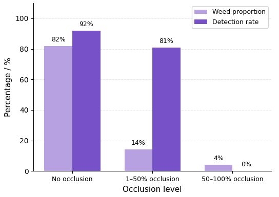
To quantify the influence of crop–weed occlusion on localization performance, the test samples were grouped according to the visibility of the weed stem or growing center, and the localization success rate was calculated separately for each occlusion level. As shown in Figure 16, non-occluded weeds accounted for 82% of the evaluated samples, with a localization success rate of 92%. Lightly to moderately occluded weeds represented 14% of the samples, for which the success rate decreased to 81%. Severely occluded weeds accounted for the remaining 4%, and no successful localization was achieved in this group because the stem base or growing center was not sufficiently visible for reliable extraction. These results show a clear decline in localization performance with increasing occlusion severity. In particular, complete or near-complete obstruction of the stem region was the main condition associated with localization failure. In the investigated maize seedling field, severely occluded weeds were typically small plants located beneath maize leaves. Such weeds had limited light availability and were difficult to access using image-guided targeted treatment. Therefore, the current method mainly focuses on visible or partially visible weed stems, which are more suitable targets for subsequent precision-weeding applications.
In addition to occlusion, weed morphology also affected localization accuracy. When weed leaves were irregular, incomplete, or strongly asymmetric, the PCA-derived principal axis could deviate from the actual stem direction, resulting in local offsets between the predicted stem center and the manually annotated ground truth. These results suggest that the proposed method is more reliable when the weed stem or growing center remains at least partially visible, but its performance may degrade in dense crop canopies, severe leaf overlap, or highly irregular weed morphology. Future work could integrate multiview image acquisition, temporal information tracking, or occlusion aware segmentation methods to further improve the robustness of weed stem localization under complex occlusion conditions.

4. Discussion

The experimental results showed that MSDNet achieved a favorable balance between maize seedling detection accuracy and model complexity. Compared with the original YOLOv8n, MSDNet increased the mAP@50 from 84.7% to 93.4% while reducing the number of parameters by 28.66%. This improvement may be attributed to the combined effects of the lightweight backbone, enhanced feature fusion, coordinate attention, and Wise-IoU loss. ShuffleNetV2 considers practical computational factors such as memory access cost and channel organization, coordinate attention preserves spatially sensitive information, and Wise-IoU reduces the adverse influence of low-quality samples during bounding-box regression. The ablation experiments further showed that these components contributed to the final detection performance.
Unlike conventional multiclass weed-recognition methods, the proposed framework first detects and excludes maize seedling regions and then extracts candidate weeds from the remaining vegetation. This strategy reduces the need for species-level weed classification and fine-grained annotation of multiple weed categories. The segmentation stage achieved an MPA of 97.6% and an mIoU of 93.8%, indicating that HSV thresholding, morphological processing, and area filtering provided sufficiently complete vegetation contours under the tested conditions. Compared with fully convolutional segmentation and stem-localization methods [33,34], the present approach requires fewer training annotations and has relatively low computational complexity. Nevertheless, fixed color thresholds may be affected by severe illumination variation, shadows, senescent vegetation, and soil regions with colors similar to vegetation.
Within the predefined 15-pixel tolerance, the proposed method achieved a weed stem detection rate of 90.1% and a localization precision of 92.5%, with a mean localization error of 10.65 pixels, corresponding to approximately 6.74 mm. Previous studies have estimated plant stems or growing points using geometric image features, fully convolutional networks, semantic graphs, and multitask networks [33,34,35]. In contrast, the present method combines crop-region exclusion with PCA and image moments and does not require point-level stem annotation during model training. Because previous studies differ in crop species, image resolution, reference-point definition, localization threshold, and evaluation metrics, direct numerical comparison should be interpreted cautiously. The present results indicate that the proposed contour-based strategy can provide effective stem localization in complex maize seedling fields while reducing annotation requirements.
The main localization errors were associated with crop–weed overlap, incomplete vegetation contours, and irregular weed morphology. PCA determines the principal axis from the overall distribution of contour pixels. Severe occlusion or asymmetric leaf distribution may therefore cause the estimated principal axis to deviate from the actual stem direction. Image-sequence information and direct keypoint learning have been used in previous studies to improve localization robustness [28,35]. Future work may combine the proposed crop-region exclusion framework with temporal information, keypoint estimation, depth sensing, or multiview imaging to improve performance under severe occlusion.
The present study represents the visual-perception and target-localization stage of a broader precision-weeding project. The proposed localization method is intended for subsequent precision-weeding applications, including laser weeding. In subsequent experiments, the method will be integrated with a laser actuator, and targeting accuracy, system delay, operating speed, weed-control efficacy, and crop safety will be evaluated under field conditions. The present findings validate the feasibility and localization performance of the proposed method and provide a technical foundation for its further application in precision weeding.

5. Conclusions

This study developed a two-stage weed stem localization method based on crop-region exclusion for maize seedling fields. MSDNet first detects maize seedlings, after which the pixel values within the detected bounding boxes are set to zero to exclude crop regions. HSV thresholding, morphological processing, and area filtering are then used to extract the remaining vegetation, and the weed stem centers are estimated by combining principal component analysis with image moments. This framework reduces dependence on multiclass weed modeling, species-specific recognition models, and point-level stem annotation.
Compared with the original YOLOv8n, MSDNet increased the mAP@50 from 84.7% to 93.4% while reducing the number of parameters from 3.21 M to 2.29 M. Vegetation segmentation achieved an MPA of 97.6% and an mIoU of 93.8%. Within a 15-pixel tolerance, corresponding to approximately 9.50 mm, the weed stem detection rate and localization precision reached 90.1% and 92.5%, respectively, with a mean localization error of 10.65 pixels, corresponding to approximately 6.74 mm. These results demonstrate the feasibility of the proposed method for image-based weed stem localization and provide visual perception and target-localization support for precision-weeding applications. The present work focuses on the visual perception and target-localization stage. Subsequent experiments will integrate the method with a laser actuator and evaluate targeting performance, weed-control efficacy, crop safety, operating speed, and system stability under field conditions.

Author Contributions

Conceptualization, Y.Z.; methodology, Y.Z.; software, Y.Z. and X.W.; validation, Y.Z.; formal analysis, Y.Z.; investigation, Y.Z. and X.W.; resources, Y.L.; data curation, X.W.; writing—original draft preparation, Y.Z.; writing—review and editing, Y.Z.; visualization, L.F.; supervision, Y.X.; project administration, Y.X.; funding acquisition, Y.X. All authors have read and agreed to the published version of the manuscript.

Funding

This research was funded by Jilin Provincial Scientific and Technological Development Program, [grant number: 20260601061RC].

Institutional Review Board Statement

Not applicable.

Data Availability Statement

The data presented in this study are available on request from the corresponding author.

Conflicts of Interest

The authors declare no conflicts of interest.

References

  1. Benvenuti, S.; Baldoni, G. Weed Flora Evolution in the Era of Climate Change: New Agronomic Issues as a Threat to Sustainable Agriculture. Agronomy 2026, 16, 764. [Google Scholar] [CrossRef] [Scilit]
  2. Blanc, L.; Lampurlanés, J.; Miquel, G.S.; Bonilla, D.P. Divergent weed control performance of wheat-legume and rapeseed-pea intercrops in conventional Mediterranean systems. Crop Prot. 2026, 208, 107670. [Google Scholar] [CrossRef] [Scilit]
  3. Cirillo, V.; Pollaro, N.; Russo, C.; Punzo, P.; Pane, M.; Maggio, A. Lack of neighbor perception in soft wheat increases weed-induced yield losses. J. Plant Physiol. 2025, 314, 154603. [Google Scholar] [CrossRef] [Scilit] [PubMed]
  4. Dhruw, J.; Victor, V.M.; Malathi, K.M. Techno Economic Evaluation of Different Types of Power Weeder in Chhattisgarh Region. J. Sci. Res. Rep. 2025, 31, 1–13. [Google Scholar] [CrossRef] [Scilit]
  5. Gagliardi, L.; Fontanelli, M.; Luglio, S.M.; Frasconi, C.; Peruzzi, A.; Raffaelli, M. Evaluation of Sustainable Strategies for Mechanical Under-Row Weed Control in the Vineyard. Agronomy 2023, 13, 3005. [Google Scholar] [CrossRef] [Scilit]
  6. Sun, D.; Chen, H.; Quan, L. Design and Experiment of Intelligent Mechanical Weeding System Based on DEM–MBD Coupling. Agriculture 2026, 16, 613. [Google Scholar] [CrossRef] [Scilit]
  7. Upadhyay, A.; Singh, K.P.; Jhala, K.B.; Kumar, M.; Salem, A. Non-chemical weed management: Harnessing flame weeding for effective weed control. Heliyon 2024, 10, e32776-. [Google Scholar] [CrossRef] [Scilit] [PubMed]
  8. Zheng, S.; Zhao, X.; Fu, H.; Tan, H.; Zhai, C.; Chen, L. Design and Experimental Evaluation of a Smart Intra-Row Weed Control System for Open-Field Cabbage. Agronomy 2025, 15, 112. [Google Scholar] [CrossRef] [Scilit]
  9. Aharon, S.; Lati, R.; Eizenberg, H.; Cohen, Y. Using planetscope imagery to evaluate herbicide efficacy in maize (Zea mays) through post-application weed detection. Precis. Agric. 2026, 27, 76. [Google Scholar] [CrossRef] [Scilit]
  10. Ge, B.; Jia, Z.; Guo, A.; Chen, W.; Wang, J.; Song, S.; Zhou, G. WeedsDetectNet: A green attention and adaptive joint feature fusion network for weed detection in agricultural fields. Crop Prot. 2026, 206, 107646. [Google Scholar] [CrossRef] [Scilit]
  11. Khan, F.; Tahir, M.N.; Aqib, M.; Lan, Y.; Zafar, N.; Saleem, S.; Haroon, Z.; Huang, W. Design and development of a low-cost industrial prototype of spot-specific spraying system for potato weed detection using deep learning. Comput. Electron. Agric. 2026, 247, 111736. [Google Scholar] [CrossRef] [Scilit]
  12. Li, W.; Zhu, W.; Wang, Q.; Gao, F.; Han, K.; Jin, X. Incorporating Crop-Centric Segmentation and Enhanced YOLOv10 for Indirect Weed Detection in Bok Choy Fields. Agronomy 2026, 16, 907. [Google Scholar] [CrossRef] [Scilit]
  13. Tan, D.; Beck, M.; Bidinosti, C.P.; Gulden, R.H.; Henry, C.J. Generative diffusion models for agricultural AI: Plant image generation, indoor-to-outdoor translation, and expert preference alignment. Comput. Electron. Agric. 2026, 249, 111862. [Google Scholar] [CrossRef] [Scilit]
  14. Li, M.; Song, X.; Zhao, Y.; Latif, A.A.A.E. Space-frequency-based multichannel dual encryption for quantum color images using chaotic system and quantum walks. Quantum Inf. Process. 2025, 24, 266. [Google Scholar] [CrossRef] [Scilit]
  15. Romeo, L.; Devanna, R.P.; Matranga, G.; Biddoccu, M.; Milella, A. Depth-aware scale normalization for robust semantic segmentation in vineyard images. Smart Agric. Technol. 2026, 14, 102161. [Google Scholar] [CrossRef] [Scilit]
  16. Subuh, A.A.; Kaboli, S.H.A.; Vallée, F. A hybrid CNN-LSTM model for accurate day-ahead wind power output forecasting with outliers detection using FCM-mahalanobis distance-ANN. E-Prime Nexus Electr. Electron. Intell. Eng. 2026, 17, 201194. [Google Scholar] [CrossRef] [Scilit]
  17. Torres, R.; Hernandez, J.; Gaweda, A.; Levinson, C.A. Leveraging artificial intelligence to personalize treatment for eating disorders: A proof-of-concept study. J. Affect. Disord. 2026, 406, 121681. [Google Scholar] [CrossRef] [Scilit] [PubMed]
  18. Wang, W.J.; Zhao, J.; Liu, H.Q.; Jiang, F. Improved inverse distance weighting with Mahalanobis distance for pose-dependent dynamics prediction in high-precision assembly robots. J. Mech. Sci. Technol. 2026, 40, 2557–2565. [Google Scholar] [CrossRef] [Scilit]
  19. Xue, S.; Li, N.; Li, Z.; Wang, D.; Zhu, T.; Jing, X.; Guo, H.; Ni, C. S2G-Net: An asymmetric cross-modal network for tiny cotton terminal-bud detection and sparse depth completion in real fields. Comput. Electron. Agric. 2026, 250, 111875. [Google Scholar] [CrossRef] [Scilit]
  20. Yu, S.J.; Ting, W.W.; Fei, Y.P.; Hao, Z. Quantum steganography scheme and circuit design based on the synthesis of three grayscale images in the HSI color space. Quantum Inf. Process. 2023, 22, 1–26. [Google Scholar] [CrossRef] [Scilit]
  21. Daraghmi, Y.A.; Naser, W.; Daraghmi, E.Y.; Fouchal, H. Drone-Assisted Plant Stress Detection Using Deep Learning: A Comparative Study of YOLOv8, RetinaNet, and Faster R-CNN. AgriEngineering 2025, 7, 257. [Google Scholar] [CrossRef] [Scilit]
  22. Sumon, S.I.; Chowdhury, M.E.H.; Chowdhury, J.U.K.; Ashraf, A.; Kashem, S.B.A.; Majid, M.E.; Nashbat, M.; Khandakar, A.; Zia, M.H.; Kunju, A.K.A. Floating waste detection using deep learning: A comparative study of YOLO, RT-DETR, and faster R-CNN. Neural Comput. Appl. 2026, 38, 293. [Google Scholar] [CrossRef] [Scilit]
  23. Zhu, P.; Li, H.; Chen, J.; Guo, C. Research on detection technology of biofouling organisms on marine aquaculture cages based on image enhancement algorithms and improved Faster R-CNN detection algorithms. Smart Agric. Technol. 2026, 14, 101419. [Google Scholar] [CrossRef] [Scilit]
  24. Dong, J.; Li, P.; Liu, J.; Qu, H.; Wang, C.; Zhang, H.; Du, D.; Bi, H.; Meng, Q. A DRCF-YOLO based method for rice seedling detection and density distribution mapping in UAV imagery. Smart Agric. Technol. 2026, 14, 102160. [Google Scholar] [CrossRef] [Scilit]
  25. Kamat, P.; Gite, S.; Chandekar, H.; Dlima, L.; Pradhan, B. Multi-class fruit ripeness detection using YOLO and SSD object detection models. Discov. Appl. Sci. 2025, 7, 931. [Google Scholar] [CrossRef] [Scilit]
  26. Liang, C.; Chen, Y.; Hu, J.; Zhou, Z. HGV-YOLO: A Detection Method for Floating Seedlings and Missed Transplanting Based on the Morphological Characteristics of Rice Seedlings. Agronomy 2026, 16, 678. [Google Scholar] [CrossRef] [Scilit]
  27. Haug, S.; Biber, P.; Michaels, A.; Ostermann, J. Plant Stem Detection and Position Estimation using Machine Vision. In Proceedings of the 2014 IEEE/RSJ International Conference on Intelligent Robots and Systems (IROS), Chicago, IL, USA, 14–18 September 2014. [Google Scholar] [PubMed]
  28. Lottes, P.; Behley, J.; Chebrolu, N.; Milioto, A.; Stachniss, C. Robust joint stem detection and crop-weed classification using image sequences for plant-specific treatment in precision farming. J. Field Robot. 2020, 37, 20–34. [Google Scholar] [CrossRef] [Scilit]
  29. Liu, M.; Xu, X.; Tian, T.; Shang, M.; Song, Z.; Tian, F.; Yan, Y. A keypoint-based method for detecting weed growth points in corn field environments. Plant Phenomics 2025, 7, 100072. [Google Scholar] [CrossRef] [Scilit] [PubMed]
  30. Zhang, X.; Li, N.; Ge, L.; Xia, X.; Ding, N. A Unified Model for Real-Time Crop Recognition and Stem Localization Exploiting Cross-Task Feature Fusion. In Proceedings of the 2020 IEEE International Conference on Real-time Computing and Robotics (RCAR); IEEE: Piscataway, NJ, USA, 2020; pp. 327–332. [Google Scholar] [CrossRef] [Scilit]
  31. Xu, L.; Hu, S.; Yang, J.; Che, Z.; Gao, X.; Pang, H.; Huang, T.; Xu, Z.; Liang, L.; Cui, M.; et al. RBSS-YOLOv8: Multi-scale feature enhancement for high-density pig aggression detection. Comput. Electron. Agric. 2026, 249, 111871. [Google Scholar] [CrossRef] [Scilit]
  32. Rekha, C.; Nagarajan, M.; Yellampalli, D.S.R.; Kumari, G.R.N. A New Automated Threat Detection Framework Using Adaptive and Multi-Head Cross Attention-Based ShuffleNetV2 for Abnormality Classification Along with Object Detection and Tracking Procedures. Cybern. Syst. 2026, 57, 694–729. [Google Scholar] [CrossRef] [Scilit]
  33. Lottes, P.; Behley, J.; Chebrolu, N.; Milioto, A.; Stachniss, C. Joint Stem Detection and Crop-Weed Classification for Plant-Specific Treatment in Precision Farming. In Proceedings of the 2018 IEEE/RSJ International Conference on Intelligent Robots and Systems (IROS), Madrid, Spain, 1–5 October 2018; pp. 8233–8238. [Google Scholar] [CrossRef] [Scilit]
  34. Bac, C.W.; Hemming, J.; Henten, E.J.v. Stem localization of sweet-pepper plants using the support wire as a visual cue. Comput. Electron. Agric. 2014, 105, 111–120. [Google Scholar] [CrossRef] [Scilit]
  35. Li, J.; Güldenring, R.; Nalpantidis, L. Real-Time Joint-Stem Prediction for Agricultural Robots in Grasslands Using Multi-Task Learning. Agronomy 2023, 13, 2365. [Google Scholar] [CrossRef] [Scilit]
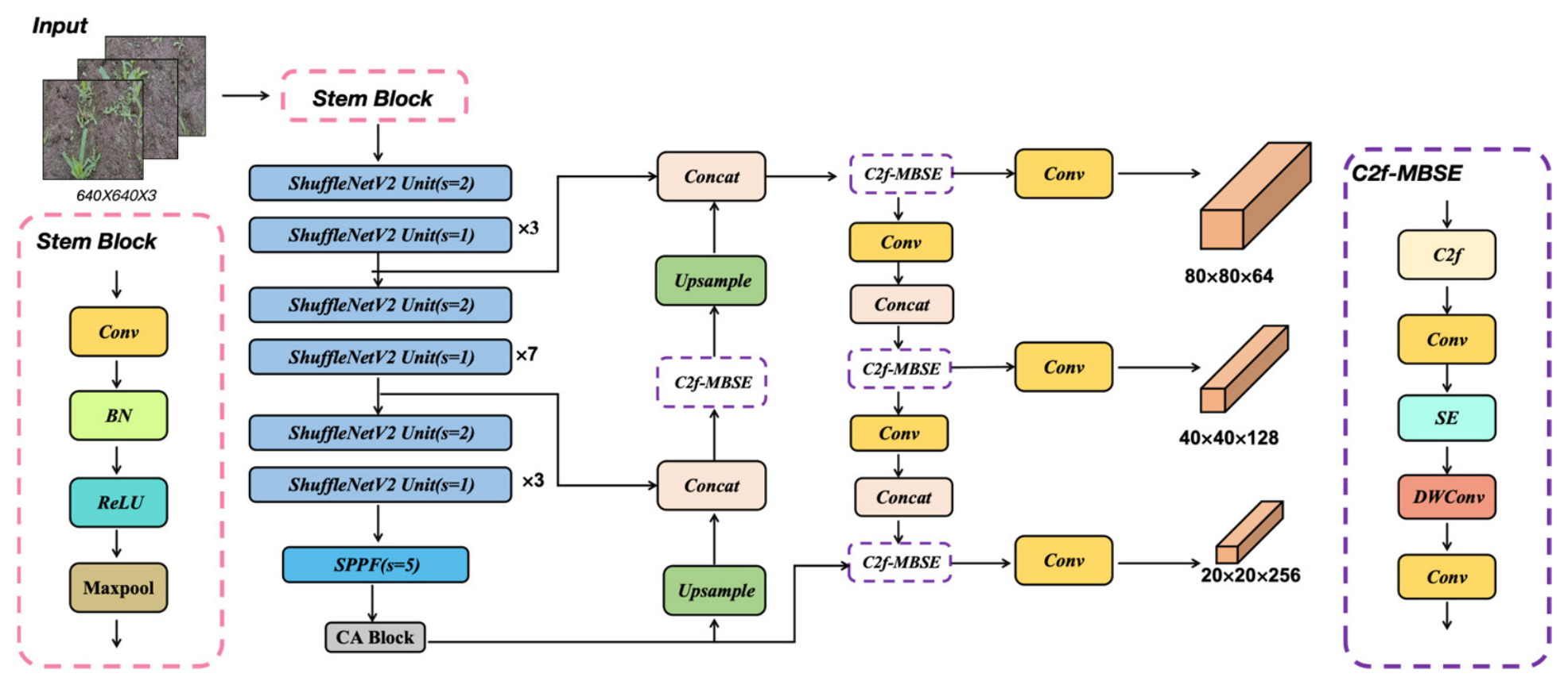
Figure 2. Network architecture of the maize detection model. Note: Conv denotes convolution; BN denotes batch normalisation; Maxpool denotes max-pooling; SFU is a lightweight feature extraction unit, where Stride = n denotes a convolution stride of n; SPPF denotes a spatial pyramid pooling module; Concat denotes tensor concatenation; SE denotes the attention mechanism module of SENet; DWConv denotes deep separable convolution.
Agronomy 16 01716 g002
Figure 3. Construction units of ShuffleNetV2. (a) Basic unit (b) Downsampling unit. Note: The ‘Channel split’ table indicates channel splitting for feature mapping; the ‘Concat’ table indicates channel concatenation; ‘Stride = 2’ indicates that the stride for depth-separable convolutions is 2.
Agronomy 16 01716 g003
Figure 4. MBConv module. Note: Conv refers to convolution; SE represents the SENet attention mechanism module; DWConv denotes depthwise separable convolution.
Agronomy 16 01716 g004
Figure 5. CA mechanism module. Note: Residual denotes the residual module; X, Y Aug Pool represents augmentation pooling in the X and Y directions; split denotes channel splitting of feature maps; Conv2d denotes two-dimensional convolution; BatchNorm denotes batch normalization; Non-linear, Sigmoid represent activation functions; C, H, W represent the length, height, and width of the channels, respectively; r represents the scaling factor.
Agronomy 16 01716 g005
Figure 6. Original image and background segmentation steps image. (a) Original image (b) Mask image (c) Preliminary segmentation results (d) Results of weed area extraction.
Agronomy 16 01716 g006
Figure 7. The process of a two-stage method for locating weed stems based on crop area exclusion.
Agronomy 16 01716 g007
Figure 8. Schematic diagram of the Euclidean distance between predicted and actual points.
Agronomy 16 01716 g008
Figure 9. Training loss and detection accuracy curves of YOLOv8n and the improved models.
Agronomy 16 01716 g009
Figure 10. HSV channel images and corresponding histograms of maize seedling field images. (a) Original image; (b) H channel; (c) S channel; (d) V channel; (e) H-channel histogram; (f) S-channel histogram; (g) V-channel histogram.
Agronomy 16 01716 g010
Figure 11. Comparative Experiment on Partitioning Algorithms.
Agronomy 16 01716 g011
Figure 12. Weed stem localization results under different maize seedling field conditions. (A1D1) Original field images; (A2D2) corresponding localization results after maize seedling region exclusion, with enlarged views of selected weed targets.
Agronomy 16 01716 g012
Figure 13. Representative results of weed stem localization. (a) Sample 1 for crop-region exclusion and weed region extraction; (b) Sample 2 for crop-region exclusion and weed region extraction. The black regions indicate the excluded maize regions, and the remaining regions are used for subsequen weed stem localization.
Agronomy 16 01716 g013
Figure 14. Boxplot-style visualization of pixel-level localization errors based on group-level average ED and standard deviation.
Agronomy 16 01716 g014
Figure 15. Typical cases affecting weed stem localization under complex field conditions. (a) Suboptimal stem localization caused by irregular weed morphology. (b) Positioning failure caused by maize occlusion interference.
Agronomy 16 01716 g015
Figure 16. Weed stem localization performance under different levels of crop–weed occlusion.
Agronomy 16 01716 g016
Table 1. Ablation experiments between different improved modules.
ModelShuffleNetV2C2f-MBSECA W I o U mAP@0.5/%Precision/%Recall/%GPU Speed/msModel Size/MBParams/M
YOLOv8n 84.790.187.81.76.33.21
Model-1 86.591.389.11.64.92.35
Model-2 89.992.190.31.86.23.05
Model-3 91.491.990.61.86.43.23
Model-4 88.793.291.11.64.72.26
Model-5 90.993.091.31.75.02.37
Model-6 91.794.292.81.96.53.17
Model-7 92.694.993.21.64.82.29
MSDNet 93.494.393.71.64.82.29
Table 2. Comparison of different lightweight backbone networks.
ModelmAP@0.5/%Precision/%Recall/%Model Size/MBParams/M
YOLOv8n84.790.187.86.33.21
EfficientNet-Lite85.986.187.95.82.84
GhostNet84.291.387.45.32.62
MobileNetV284.489.687.95.82.71
MobileNetV385.890.688.75.22.56
ShuffleNetV286.591.389.14.92.35
Table 3. Comparison of segmentation algorithm performance.
Segmentation AlgorithmMPA/%mIoU/%Average Processing Time/s
G-channel thresholding + OTSU84.676.60.07
H-channel thresholding + OTSU89.782.40.05
HSV thresholding + morphological processing97.693.80.08
Table 4. Sensitivity analysis of HSV threshold settings.
SettingH-RangeMPA/%mIoU/%Green Area Ratio/%
HSV-1[30, 60]96.892.618.9
HSV-2[32, 58]97.293.118.1
HSV-3 Original[35, 55]97.693.817.4
HSV-4[38, 52]97.193.016.6
HSV-5[40, 50]96.491.915.8
Table 5. Weed stem localization results under different field images.
ImagesCategory
A 2B 2C 2D 2
The number of weeds/unit20132936
Number of annotated bounding boxes/unit18132632
Number of misclassifications/unit0000
Number of misses/unit2034
Miss rate/%10%0%10.34%11.11%
Accuracy of marking/%90%100%89.66%88.89%
Table 6. Quantitative evaluation of weed stem localization accuracy.
NumbersNumbers of Weeds Stems/PlantP/%D/%M/%Average ED/PixelStandard Deviation/PixelsRMSE/PixelMAE/Pixel
Group 17291.488.911.19.84.312.0210.65
Group 216393.790.89.29.14.9
Group 324892.291.18.910.65.8
Group 435692.590.29.811.85.9
Group 544792.889.910.110.25.3
Group 651192.389.610.410.95.6
Disclaimer/Publisher’s Note: The statements, opinions and data contained in all publications are solely those of the individual author(s) and contributor(s) and not of MDPI and/or the editor(s). MDPI and/or the editor(s) disclaim responsibility for any injury to people or property resulting from any ideas, methods, instructions or products referred to in the content.