High-Resolution Soil Organic Carbon Mapping with Interpretability and Uncertainty Quantification in Hungarian Croplands

Abstract

Accurate prediction of soil organic carbon (SOC) at fine resolution is crucial for precision soil management; however, existing national products for Hungary remain too coarse for farm-scale applications. Focusing on Hungarian croplands, we developed a 30 m resolution SOC map using multi-temporal bare-soil composites, DEM derivatives, SHAP interpretability and bootstrap uncertainty. Among five evaluated algorithms, the GBDT model achieved the best performance (test R² = 0.518, RMSE = 4.498 g·kg⁻¹, MAE = 3.499 g·kg⁻¹, RPIQ = 2.229, LCCC = 0.621). SHAP analysis revealed pronounced nonlinear effects of spectral and topographic variables within this modeling framework, with spectral predictors playing a dominant role in SOC prediction. Furthermore, the bootstrap uncertainty framework yielded a Prediction Interval Coverage Probability of 94.59% at the 95% confidence level, indicating reliable interval estimation for the test set. Spatial patterns of uncertainty varied considerably, with higher values in the western hills and southern sands, and moderate levels in the northern low-mountain areas. Benchmark comparisons showed that our 30 m map captures fine-scale heterogeneity often smoothed over by coarser products, while the uncertainty layer supports risk-aware interpretation. Overall, this study provides a regionally calibrated framework for mapping in similar heterogeneous agricultural landscapes, providing practical insights for local management.

1. Introduction

Soil organic carbon (SOC) is a pivotal indicator of cropland soil fertility and health, directly dictating nutrient retention, soil structure, water-holding capacity, and, ultimately, crop productivity [1]. Consequently, spatially explicit SOC maps are essential for monitoring regional soil quality and safeguarding farmland productivity [2]. High-resolution spatial predictions of SOC accurately capture its distribution and spatial variability, providing a critical foundation for precision fertilization, conservation tillage zoning, and sustainable agricultural development strategies.

Although traditional soil sampling yields accurate point measurements, it fails to capture spatially continuous SOC dynamics across large extents. Remote sensing has emerged as an effective alternative by leveraging soil–spectral relationships [3,4,5]. Recent methodological advances have helped shift SOC mapping from linear regression and partial least squares to machine learning algorithms that better accommodate complex, nonlinear interactions. However, because model performance is highly contingent on regional environmental contexts, the success of region-specific methodologies cannot be directly extrapolated to diverse soil–landscape settings. In Hungary, accurate, high-resolution SOC maps remain largely unavailable. Existing national mapping efforts, notably those leveraging the Hungarian Soil Information and Monitoring System (SIMS) database—including recent implementations of quantile regression forests [6] and spatiotemporal machine learning combined with space–time geo-statistics [7]—remain limited to a 100 m resolution. Meanwhile, LUCAS-derived gridded products range from 500 m to 1 km [8], and SoilGrids offers a 250 m resolution [9]. These products are all too coarse to resolve the within-field SOC heterogeneity essential for precision farm-scale management. The 30 m resolution of Landsat imagery represents a practical intermediate scale, bridging the gap between coarse regional products (≥100 m) and very-high-resolution data (<5 m) that are often cost-prohibitive for wall-to-wall national coverage. Although recent advances in bare-soil compositing and machine learning have demonstrated the feasibility of 30 m SOC mapping in other agricultural regions, such an approach has not yet been calibrated or validated for Hungary’s heterogeneous cropland mosaic.

Generating a finer-resolution map requires modeling frameworks capable of capturing the complex, nonlinear relationships between SOC and its spectral–topographic predictors. Machine learning algorithms, such as random forest (RF), support vector machines (SVM), and Extreme Gradient Boosting (XGBoost), have been widely adopted due to their proficiency in modeling nonlinear interactions and delivering high predictive accuracy [10]. Nevertheless, model efficacy is inherently tied to regional contexts, necessitating region-specific calibrations [11]. Furthermore, the “black-box” nature of machine learning algorithms limits geoscientific explainability [12]. This limitation motivates the adoption of post hoc explanation frameworks like SHAP, which decomposes predictions into per-predictor contributions and reveals threshold responses, thereby clarifying the mechanisms driving spatial SOC heterogeneity [13,14]. Assessing prediction uncertainty is equally critical; in regions characterized by long-tailed SOC distributions and weak spectral signals, a single deterministic map can obscure substantial local prediction errors [15]. Among available uncertainty quantification techniques—including Bayesian inference, Monte Carlo dropout, and quantile regression forests—bootstrap resampling offers a computationally efficient, distribution-free approach for pixel-scale uncertainty estimation [9,16], systematically highlighting areas where predictions exhibit lower reliability.

Despite the availability of national SOC products for Hungary, three critical gaps remain: (1) there is currently no 30 m resolution SOC map for Hungarian croplands capable of supporting farm-scale precision management; (2) a mechanistic understanding of how spectral and topographic variables nonlinearly govern SOC distribution is lacking; and (3) the uncertainty of fine-scale predictions has not been systematically quantified across Hungary’s diverse terrains—ranging from flat plains to hilly and low-mountain areas—leaving end-users without guidance regarding map reliability. To address these gaps, this study tests three hypotheses: (H1) nonlinear ensemble methods, particularly gradient boosting, may be more effective than linear models and regularized alternatives in capturing the complex SOC–environment relationships within Hungary’s heterogeneous croplands; (H2) both spectral and topographic covariates are expected to show significant nonlinear threshold effects on SOC, and their marginal responses could be quantitatively characterized via SHAP-based diagnostics in this context; and (H3) prediction uncertainty is likely to increase alongside terrain complexity, potentially enabling the proposed 30 m map to reveal fine-scale spatial heterogeneity that may be otherwise smoothed over in coarser benchmark products.

The primary aim of this study is to develop an interpretable, region-specific framework to produce the first dedicated 30 m resolution SOC map for Hungarian croplands, complete with pixel-wise uncertainty assessments. This research pursues three interconnected objectives: (1) to execute a rigorous model intercomparison—incorporating spatial block cross-validation and temporal window evaluation—to ensure robust spatial generalization; (2) to apply SHAP analysis as a diagnostic tool for quantifying the nonlinear threshold responses of SOC to environmental covariates, while simultaneously utilizing bootstrap-based uncertainty quantification to map prediction reliability; and (3) to perform a systematic comparison against existing benchmark SOC products using multi-dimensional diagnostics, thereby elucidating the added value of fine-scale mapping for farm-scale applications. The subsequent sections detail the data sources, preprocessing procedures, and the modeling framework utilized to operationalize this approach. By fulfilling these objectives, this study delivers a reliable, high-resolution SOC map for Hungary and provides a regionally calibrated reference for SOC mapping in analogous heterogeneous agricultural landscapes.

2. Materials and Methods

2.1. Study Area

The study area encompasses Hungary, located in Central Europe between latitudes 45°48′–48°35′ N and longitudes 16°05′–22°58′ E (Figure 1a). Hungary covers a total land area of 93,023 km², with agricultural land accounting for 55.3% of its surface [17]. The region experiences a temperate continental climate, with a mean annual temperature of 10–11 °C and mean annual precipitation of approximately 630 mm. Situated within the Carpathian Basin, Hungary exhibits distinct topographical variations (Figure 1b): the flat Great Hungarian Plain dominates the central and eastern regions, gentle rolling hills characterize the west, and low mountains align along the northern border. Cropland elevation generally ranges from 70 m to 300 m above sea level. Pedologically, the plains are predominantly dominated by fertile Chernozems and SOC-rich meadow soils, whereas Luvisols and Cambisols prevail in the surrounding hilly and mountainous terrains [18]. Hungary has a long-established agricultural sector, with winter wheat, maize, and sunflower as the primary crops. The interaction between the continental climate and local management practices creates two distinct bare-soil exposure windows: prior to spring sowing (March–May) and following autumn tillage (September–November). These temporal windows provide optimal conditions for acquiring high-quality, cloud- and vegetation-free Landsat 8 imagery for accurate SOC mapping.

2.2. Data Sources and Preprocessing

2.2.1. Soil Sampling Data

Soil organic carbon (SOC) data for this study were obtained from the 2015 topsoil database of the Land Use/Cover Area frame Survey (LUCAS) (Figure 1). Coordinated by Eurostat and the Joint Research Centre (JRC), the LUCAS program employs a rigorous stratified systematic sampling design. Across Europe, topsoil samples (0–20 cm) were collected, and their SOC content ($\mathrm{g}\cdot {\mathrm{kg}}^{-1}$) was quantified via dry combustion within a single ISO-certified laboratory [19]. This highly standardized protocol effectively mitigates inter-laboratory systematic errors, ensuring high reliability of the baseline dataset. To minimize the adverse impacts of potential sampling or analytical anomalies on model training, the initial cropland dataset ($n=261$) was screened using the three-sigma ($3\sigma$) rule. Consequently, two extreme outliers deviating substantially from the primary distribution were identified and removed, yielding a refined dataset of 259 valid samples for subsequent modeling.

2.2.2. Box–Cox Transformation and Smearing Bias Correction

To address the right-skewed distribution of SOC data and stabilize variance, a Box–Cox transformation was applied to the target variable following the train-test split [20]. To strictly prevent data leakage, the transformation parameter $\lambda$ was estimated exclusively from the training set and subsequently applied to the independent test set. All predictive models were then trained using the transformed SOC values as the response variable. Upon back-transformation to the original scale, the standard inverse Box–Cox function yields conditional median rather than conditional mean predictions; for positively skewed SOC distributions, this inherently results in systematic underestimation in high-value regions. To obtain approximately unbiased mean predictions on the original measurement scale, the Duan smearing estimator was employed [21]. Specifically, empirical residuals were computed from the training data in the transformed space. For each prediction, the smearing-corrected estimate was derived by averaging the inverse-transformed values obtained after adding back each individual training residual. These bias-corrected predictions were utilized for all subsequent performance evaluations on the test set.

2.2.3. Compositing Bare-Soil Image from Multi-Temporal Landsat 8 Data

The Landsat 8 Collection 2 Tier 1 surface reflectance (SR) product, featuring a 30 m spatial resolution, was utilized for bare-soil compositing in this study. Generated by the U.S. Geological Survey (USGS), this product is atmospherically corrected using the Land Surface Reflectance Code (LaSRC) algorithm and certified as Analysis Ready Data (ARD) by the Committee on Earth Observation Satellites (CEOS) [7]. It provides six multispectral bands (B2–B7) spanning the 0.452–2.294 $\mathsf{\mu }\mathrm{m}$ wavelength range—encompassing the visible, near-infrared, and shortwave infrared regions—alongside a Quality Assessment (QA) band employed to identify and mask clouds, cloud shadows, and snow. The data are stored as 16-bit integer GeoTIFF files, with true surface reflectance derived via the scaling equation:

$$reflectance=DN \times 2.75 \times {10}^{-5}-0.2$$

(1)

where $\mathrm{reflectance}$ represents the dimensionless surface reflectance (typically ranging from 0 to 1), and $\mathrm{DN}$ denotes the digital number stored within the 16-bit GeoTIFF files. Validation assessments over bare soil and desert surfaces demonstrate that the Landsat 8 SR product exhibits atmospheric correction errors below 4% in the shortwave infrared and near-infrared bands, confirming its suitability for bare-soil spectral retrieval and subsequent soil property estimation [22].

To identify the optimal temporal window for bare-soil compositing, all available Landsat 8 SR images acquired during Hungary’s bare-soil phenological windows (March–May and September–November) were collected via Google Earth Engine (GEE). The data were grouped into two independent temporal windows: 2013–2018 and 2016–2020. The 2013–2018 window was centered around the 2015 LUCAS sampling year ($\pm 2$ years), whereas the 2016–2020 window provided a more recent, denser set of observations with enhanced temporal continuity. Initial preprocessing involved masking clouds, cloud shadows, and saturated pixels using the QA band, after which surface reflectance values were derived using official scale factors and offsets.

To delineate cropland extent, 10 m resolution land cover tiles of Hungary from the Copernicus Land Monitoring Service (CLMS) [23] were mosaicked to generate a seamless map. To ensure spatial compatibility with Landsat 8 imagery, this dataset was reprojected to the WGS 84 coordinate reference system and resampled to 30 m resolution. The resulting map was reclassified into a binary raster, where cropland pixels were assigned a value of 1 and all non-cropland cover types were aggregated to 0. This binary mask was integrated into GEE, where a dual-threshold rule ($\mathrm{NDVI}<0.25$ and $\mathrm{BSI}>0$) was applied to remove residual non-bare-soil pixels, effectively isolating bare soil within croplands [24].

To maximize cloud-free bare-soil spatial coverage, observations from both spring and autumn phenological windows were integrated. For each temporal period, a pixel-wise median composite was generated across the multi-temporal image stack to extract a stable baseline surface reflectance. The selection of the median estimator stems directly from its ability to suppress interference from anomalous outliers, transient vegetation, and residual surface moisture, yielding a bare-soil spectral signal with a degree of robustness against transient artifacts that the arithmetic mean cannot provide [25]. Finally, the two resulting composite images (2013–2018 and 2016–2020) were used independently to train five machine learning models under identical configurations (Section 2.3). Based on predictive performance on the independent test set (Section 3.5), the 2016–2020 composite (Figure 2) demonstrated superior accuracy and was selected as the baseline input for final SOC mapping, SHAP interpretation, and uncertainty analysis.

2.2.4. Derivation of the Spectral and Topographic Variables

Predictor variables were derived from two primary sources: spectral features extracted from the bare-soil composites and topographic metrics derived from the Copernicus DEM GLO-30. The spectral feature suite comprises six primary reflectance bands (Blue, Green, Red, NIR, SWIR1, and SWIR2) and seven spectral indices, including the Normalized Difference Vegetation Index (NDVI), Soil-Adjusted Vegetation Index (SAVI), Bare Soil Index (BSI), and Normalized Red–Green Difference Index (NRGDI) (

Table 1. Predictor variables used for SOC content spatial prediction: abbreviations, definitions, and calculations.

Category	Feature Name	Abbreviation	Definition/Calculation
Topographic factors	Elevation	H	Bare-earth terrain height
	Slope	Slope	First derivative of elevation
	Aspect	Aspect	Direction of the maximum slope
	Profile Curvature	Prof_Curv	Curvature parallel to the direction of maximum slope
	Plan Curvature	Plan_Curv	Curvature perpendicular to the direction of maximum slope
Hydro-Morphological factors	Topographic Wetness Index	TWI	$\ln \mathrm{(}\mathrm{\alpha }\mathrm{/}\tan \mathrm{\beta }\mathrm{)}$
	Topographic Position Index	TPI	Difference between central pixel and mean neighborhood elevation
	Terrain Ruggedness Index	TRI	Root mean square of elevation differences
	Valley Depth	VD	Vertical distance to the channel base
	Multiresolution Index of Valley Bottom Flatness	MrVBF	Identification of valley bottoms based on multi-scale slope
	Multiresolution Index of Ridge Top Flatness	MrRTF	Identification of ridge tops based on multi-scale slope
Spectral bands	Blue, Green, Red	B2, B3, B4	Visible reflectance during the bare-soil period
	Near Infrared	B5	NIR reflectance during the bare-soil period
	Shortwave Infrared 1, 2	B6, B7	SWIR reflectance during the bare-soil period
Spectral indices	Normalized Difference Vegetation Index	NDVI	(B5 − B4)/(B5 + B4)
	Soil-Adjusted Vegetation Index	SAVI	$\mathrm{\left[}\mathrm{\right(}\mathrm{B}\mathrm{5}\mathrm{-}\mathrm{B}\mathrm{4}\mathrm{)}\mathrm{/}\mathrm{(}\mathrm{B}\mathrm{5}\mathrm{+}\mathrm{B}\mathrm{4}\mathrm{+}\mathrm{L}\mathrm{\left)}\mathrm{\right]}\mathrm{\times }\mathrm{(}\mathrm{1}\mathrm{+}\mathrm{L}\mathrm{)}$
	Bare Soil Index	BSI	[(B6 + B4) − (B5 + B2)]/[(B6 + B4) + (B5 + B2)]
	Normalized Red–Green Difference Index	NRGDI	(B4 − B3)/(B4 + B3)
	Normalized Difference Moisture Index	NDMI	(B5 − B6)/(B5 + B6)
	Brightness Index	BI	sqrt((B42 + B32)/2)
	Ratio Vegetation Index	RVI	(B5/B4)

). To capture terrain influences, the 30 m resolution Copernicus DEM GLO-30 was utilized. Generated from TanDEM-X interferometric radar data acquired between 2010 and 2015 [26], this DEM was hydrologically conditioned via water surface flattening and stream burning to optimize terrain analysis [27]. Primary topographic factors—specifically elevation, slope, aspect, plan curvature, and profile curvature—were computed from the conditioned DEM. Additionally, a comprehensive set of hydro-topographic variables were extracted, encompassing the Topographic Wetness Index (TWI), Topographic Position Index (TPI), Terrain Ruggedness Index (TRI), Valley Depth, Multiresolution Index of Valley Bottom Flatness (MrVBF), and Multiresolution Index of Ridge Top Flatness (MrRTF). All spectral and topographic variables were computed within Google Earth Engine (GEE) using standard median compositing and terrain analysis routines. Detailed definitions and calculation formulas for all predictor variables are provided in Table 1.

2.3. Machine Learning Methods and Hyperparameter Optimization

Five machine learning algorithms representing distinct statistical paradigms were evaluated: partial least squares regression (PLS) as a linear baseline, support vector machines (SVM) utilizing a radial basis function (RBF) kernel for nonlinear regression, random forest (RF) as a bagging ensemble, and two gradient-boosting frameworks—gradient boosting decision trees (GBDT) and Extreme Gradient Boosting (XGBoost). This selection spans both linear dimensionality reduction techniques and nonlinear ensemble architectures capable of accommodating high-dimensional, spatially heterogeneous environmental data. Given the moderate training sample size ($n=207$ following the split), a parsimonious hyperparameter search strategy was adopted to balance model complexity against overfitting risks. Hyperparameters for each algorithm were optimized via an exhaustive grid search coupled with 10-fold cross-validation on the training set, prioritizing cross-validated $R^2$, followed by root mean square error (RMSE) [28,29,30,31,32]. The tuned hyperparameters included: the number of latent variables for PLS; the penalty parameter ($C$) and kernel width ($\gamma$) for SVM; tree count, maximum depth, and maximum features per split for RF; learning rate, boosting stages, and maximum tree depth for GBDT; and L2 regularization weight and minimum loss reduction for XGBoost. Upon identifying the optimal hyperparameter configurations, all five models were retrained on the full training dataset. The independent test set was reserved strictly for final, unbiased performance evaluation. Ultimately, the top-performing model derived from this intercomparison was selected for subsequent SHAP-based interpretability analysis and bootstrap-based uncertainty quantification.

2.4. Model Performance Assessment

The 259 soil samples were partitioned into training (80%) and testing (20%) sets via quintile-based stratified random sampling across five SOC strata, ensuring distributional equivalence between subsets. Five complementary evaluation metrics—the coefficient of determination ($R^2$), root mean square error ($\mathrm{RMSE}$), mean absolute error ($\mathrm{MAE}$), ratio of performance to interquartile distance ($\mathrm{RPIQ}$), and Lin’s concordance correlation coefficient ($\mathrm{LCCC}$)—were employed to assess the predictive accuracy and generalization capacity of each model:

$$R^2=1-{\displaystyle \frac{{\displaystyle {\sum }_{i=1}^n{(y_i-{\widehat{y}}_i)}^2}}{{\displaystyle {\sum }_{i=1}^n{(y_i-{\overline{y}}_i)}^2}}}$$

(2)

$$RMSE = \sqrt{{\displaystyle \frac{1}{n}}{\displaystyle {\sum }_{i=1}^n{(y_i-{\widehat{y}}_i)}^2}}$$

(3)

$$MAE = {\displaystyle \frac{1}{n}}{\displaystyle {\sum }_{i=1}^n\left|y_i-{\widehat{y}}_i\right|}$$

(4)

$$RPIQ = {\displaystyle \frac{Q_3-Q_1}{RMSE}}$$

(5)

$$LCCC = {\displaystyle \frac{2\rho {\sigma }_y{\sigma }_{\widehat{y}}}{{\sigma }_y^2+{\sigma }_{\widehat{y}}^2+{(\overline{y}-\overline{\widehat{y}})}^2}}$$

(6)

where $y_i$ and ${\widehat{y}}_i$ are the measured and predicted values for the $i$-th sample, and $n$ is the total number of samples; $Q_1$ and $Q_3$ are the first (25%) and third (75%) quartiles of the measured SOC data, respectively; $r$ is the Pearson correlation coefficient between measured and predicted values; ${\sigma }_y^2$ and ${\sigma }_{\widehat{y}}^2$ (or ${\sigma }_y$ and ${\sigma }_{\widehat{y}}$) denote the variances and standard deviations of measured and predicted values; and $\overline{y}$ and $\overline{\widehat{y}}$ represent their respective means. Specifically, $R^2$ quantifies the proportion of spatial variance explained by the model, bounded within $\left[0,1\right]$, where higher values indicate superior fit. $\mathrm{RMSE}$ assesses overall predictive precision and is sensitive to large residual errors, with lower values reflecting greater absolute accuracy. $\mathrm{MAE}$ measures the mean absolute magnitude of residuals, providing a robust assessment of average prediction error. $\mathrm{RPIQ}$—defined as the interquartile range ($\mathrm{IQR}=Q_3-Q_1$) divided by $\mathrm{RMSE}$—evaluates model consistency relative to dataset dispersion, where higher values denote enhanced predictive capacity across the data spectrum [33]. Finally, $\mathrm{LCCC}$ evaluates direct concordance between predicted and measured values by simultaneously accounting for linear correlation and systematic bias relative to the 1:1 identity line. Bounded within $\left[-1,1\right]$, an $\mathrm{LCCC}$ value approaching 1 indicates both high linear correlation and strong alignment along the 1:1 concordance line [34].

To mitigate spatial autocorrelation among the 259 soil samples and address regional geographic heterogeneity, conventional random cross-validation was eschewed, as it tends to yield overly optimistic performance estimates due to spatial data leakage. To rigorously evaluate the spatial generalization capacity of the models, a spatial block cross-validation (Spatial Block CV) scheme was implemented. The study area was partitioned into geographically distinct blocks using coordinate-based $k$-means clustering. Specifically, the region was divided into 10 spatial blocks, each containing approximately 25–30 samples. Models were iteratively trained on a subset of blocks and evaluated on the remaining independent geographic blocks, ensuring that training and validation samples were sufficiently separated in geographic space. To further assess whether the prediction residuals of the optimal model—identified from the five-algorithm intercomparison—retained spatial dependency, global Moran’s $I$ was computed on the residuals using $K$-nearest neighbor spatial weight matrices ($K=5,7, \mathrm{and} 10$), with statistical significance evaluated via 9999 Monte Carlo permutations.

2.5. SHAP-Based Model Explanation

To quantify the influence of individual environmental predictors on the spatial distribution of topsoil soil organic carbon (SOC), the SHapley Additive exPlanations (SHAP) framework was employed. Rooted in cooperative game theory, SHAP provides additive feature attributions by computing the average marginal contribution of each variable across all possible feature subsets [35]. The local explanation model is defined as follows:

$$g(z\prime ) = {\varphi }_0+{\displaystyle \sum _{j=1}^M{\varphi }_j}z{\prime }_j$$

(7)

where $g$ is the explanation model; $z^{\prime }\in {\left\{0,1\right\}}^M$ is a binary vector indicating feature inclusion in the coalition; $M$ is the total dimension of the input prediction variables; ${\varphi }_0$ is the baseline prediction when no features are included; and ${\varphi }_j$ represents the SHAP marginal contribution of the $j$-th prediction variable. The sign of ${\varphi }_j$ indicates the direction of influence exerted by the corresponding environmental factor on the model prediction: ${\varphi }_j>0$ denotes a positive effect on SOC accumulation, whereas ${\varphi }_j<0$ signifies a negative effect.

SHAP values were calculated for all independent test samples using the best-performing model. For global model interpretation, the mean absolute SHAP value of each predictor variable was computed to establish a global feature importance ranking, thereby identifying the primary environmental drivers shaping spatial SOC patterns across the study area [35]. For local model interpretation, SHAP dependence plots were constructed for the top-ranked predictors. These plots illustrate the nonlinear responses of predicted SOC to variations in individual covariates, facilitating the identification of critical threshold effects and interactions between spectral and topographic variables [36]. By shifting the analytical focus from purely data-driven mapping toward a mechanistic understanding, this approach illuminates how environmental covariates govern spatial SOC heterogeneity.

2.6. Bootstrap-Based Spatial Uncertainty Quantification

To quantify the spatial uncertainty of SOC predictions, a bootstrap-based framework was implemented by generating 100 bootstrap resamples for model training [16]. The pixel-wise standard deviation (SD) and coefficient of variation (CV) were calculated across the 100 bootstrap predictions to assess model stability. To evaluate whether these estimated uncertainty bounds reflect true prediction reliability rather than merely resampling variability, the Prediction Interval Coverage Probability (PICP) and Mean Prediction Interval Width (MPIW) were computed at a 95% confidence level using the independent test set. PICP measures the proportion of observed values falling within the bootstrap-derived 95% prediction intervals, whereas MPIW quantifies the average width of these intervals. A reliable uncertainty framework should yield a PICP close to the nominal 95% target while maintaining a narrow, physically meaningful MPIW.

2.7. Comparison with Existing SOC Products

To contextualize the predictions within the existing geospatial product landscape, a systematic comparison was conducted against three authoritative benchmark SOC maps selected based on public accessibility, dataset authority, and relevance to topsoil SOC content (Figure 3a–c). SERENA 2016 (100 m resolution) was chosen as the primary national benchmark due to its close temporal proximity to the 2015 LUCAS sampling campaign; this product was generated via random forest kriging using the Hungarian Soil Information and Monitoring System (SIMS) database alongside environmental covariates [37] and is accessible via Zenodo [38]. SoilGrids 2.0 (250 m resolution) [9] served as the global SOC benchmark, whereas Szatmári et al. (2024) [6] provided a 100 m resolution national historical baseline representing SOC conditions circa 2000 (approximately 15 years prior to the 2015 LUCAS sampling). Although this temporal offset represents an inherent constraint of the comparison, no temporal harmonization was attempted due to the absence of intermediate validation data. Alternative candidate products (e.g., HU-SoilCarbonGrids, HoliSoils, and CUP4SOIL) were excluded owing to data inaccessibility, incompatible target variables, or land cover mismatches.

For analytical consistency, all benchmark rasters were reprojected and resampled to a common 30 m grid (EPSG:32634) using bilinear interpolation, masked to cropland areas using the CORINE land cover dataset [39], and spatially aligned with our prediction map. Because SoilGrids 2.0 provides SOC predictions across discrete depth intervals, its 0–5 cm, 5–15 cm, and 15–30 cm layers were aggregated into a unified 0–30 cm depth interval using the trapezoidal rule [40]. In contrast, SERENA 2016 and Szatmári et al. were evaluated without depth conversion, as they natively represent the 0–30 cm soil layer. Notably, while our prediction map specifically targets the 0–20 cm depth interval, all three benchmark products cover 0–30 cm. Depth harmonization was intentionally omitted; instead, this systematic discrepancy is interpreted in the discussion (Section 4.5).

Uncertainty layers were excluded from direct quantitative comparison because their underlying uncertainty quantification frameworks differ fundamentally across products. SoilGrids 2.0 defines uncertainty as the difference between the 95th and 5th percentiles derived from quantile regression forests; Szatmári et al. [6] report 90% prediction intervals derived from kriging variance; and SERENA 2016 lacks a publicly available uncertainty layer. In contrast, our uncertainty map was generated using a bootstrap-based framework (100 resamples), yielding distinct operational definitions and scales of uncertainty. Consequently, a direct numerical comparison of these spatial uncertainty layers would be methodologically inconsistent and potentially misleading.

All benchmark rasters were reprojected to a common 30 m grid (EPSG:32634) using bilinear interpolation, masked to cropland extents using the CORINE land cover dataset, and spatially aligned with the proposed prediction map. Following the spatial raster comparison framework proposed by Nowosad [41], pixel-wise difference maps—calculated as the proposed prediction minus each benchmark—were generated, and their corresponding histograms were inspected to identify patterns of over- and under-prediction. Spatial autocorrelation in these biases was assessed by calculating global Moran’s $I$ for the difference raster relative to SERENA. Furthermore, local-scale agreement was quantified using the focal Pearson correlation coefficient within a $5\times 5$ moving window. While the global Pearson correlation captures overall agreement in macro-spatial trends, the focal correlation assesses local structural congruence, distinguishing whether the maps share fine-scale details beyond mean offsets.

Quantitative agreement was evaluated using the Pearson correlation coefficient ($r$), root mean square error ($\mathrm{RMSE}$), bias, and Lin’s concordance correlation coefficient ($\mathrm{LCCC}$) [34]. Systematic biases were further characterized via Reduced Major Axis (RMA) regression [42] and the Bland–Altman analysis [43]. To illustrate the resolution advantages of the proposed 30 m product, representative sub-regions were extracted and visualized at their native spatial resolutions, facilitating a direct qualitative comparison of spatial detail and boundary sharpness. Additionally, to investigate the drivers of observed bias, the relationship between prediction error (proposed map minus SERENA) and elevation was analyzed, with bias distributions summarized across five elevation zones defined by natural breaks [44].

A control experiment was conducted to evaluate whether incorporating macro-scale climatic and parent material covariates—theoretically relevant to SOC but available only at coarser resolutions—would improve model performance. Specifically, an expanded covariate set including mean annual temperature, mean annual precipitation, and categorical parent material was evaluated against the core framework to determine whether these data enhance predictive power or, conversely, degrade performance due to spatial mismatch and information dilution during 30 m upscaling. All analyses were implemented in Python 3.14 utilizing the rasterio, numpy, scipy, scikit-learn, libpysal/esda, and matplotlib libraries. The stability of all primary performance metrics was verified through bootstrap resampling ($\mathrm{CV}<0.5\%$).

3. Results

3.1. Descriptive Statistics and Dataset Partition

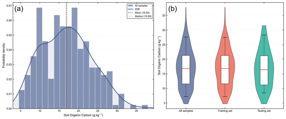
Descriptive statistics for the 259 valid soil samples—retained after excluding two extreme outliers using the 3$\sigma$ rule—are summarized in

Table 2. Descriptive statistics of cropland topsoil SOC content for the full, training, and test datasets.

Dataset	N	Min (g·kg−1)	Max (g·kg−1)	Mean (g·kg−1)	Median (g·kg−1)	SD (g·kg−1)	CV (%)	Skewness	Kurtosis
Train	207	4.70	37.80	16.97	16.80	6.43	37.90	0.28	−0.35
Test	52	4.70	31.50	16.79	16.40	6.54	38.98	0.35	−0.49
All data	259	4.70	37.80	16.93	16.80	6.44	38.04	0.29	−0.40

. The soil organic carbon (SOC) content ranged from 4.70 to 37.80 $\mathrm{g}\cdot {\mathrm{kg}}^{-1}$, with a mean of 16.93 $\mathrm{g}\cdot {\mathrm{kg}}^{-1}$ and a median of 16.80 $\mathrm{g}\cdot {\mathrm{kg}}^{-1}$. A coefficient of variation (CV) of 38.04% indicates moderate-to-high spatial heterogeneity. With a skewness of 0.29 and a kurtosis of −0.40, the dataset exhibits an approximately symmetric, slightly platykurtic distribution (Figure 4a). To ensure representative model training and evaluation, the samples were partitioned via quantile-based stratified random sampling across five strata defined by SOC quintiles. Approximately 80% of the samples ($N=207$) were allocated to the training set, while the remaining 20% ($N=52$) were reserved for independent testing. The training set exhibited a mean SOC of 16.97 $\mathrm{g}\cdot {\mathrm{kg}}^{-1}$ ($\mathrm{CV}=37.90\%$), whereas the test set displayed a mean of 16.79 $\mathrm{g}\cdot {\mathrm{kg}}^{-1}$ ($\mathrm{CV}=38.98\%$). Visual inspection of the violin plot (Figure 4b) confirms distributional similarity between the two subsets, a finding corroborated by the Kolmogorov–Smirnov (K–S) test ($D=0.069$, $p=0.979$). These results confirm the efficacy of the stratified sampling strategy, ensuring distributional equivalence for robust assessment of model generalization.

3.2. Model Performance and Accuracy Assessment

To mitigate the mild positive skewness observed in the raw soil organic carbon (SOC) data ($\mathrm{skewness}=0.29$), a Box–Cox transformation was applied prior to model training, with the optimal transformation parameter $\lambda$ estimated via maximum likelihood estimation (Section 2.2.2). Following model inference, Duan’s smearing estimator was employed to back-transform all predicted values onto the original SOC scale [21]. Consequently, the performance evaluation metrics reported in

Table 3. Performance comparison of five machine learning models.

Model	Dataset	${\mathit{R}}^2$	$\mathit{R}\mathit{M}\mathit{S}\mathit{E}$ ($\mathbf{g}·{\mathbf{k}\mathbf{g}}^{-1}$)	$\mathit{M}\mathit{A}\mathit{E}$ ($\mathbf{g}·{\mathbf{k}\mathbf{g}}^{-1}$)	$\mathit{R}\mathit{P}\mathit{I}\mathit{Q}$	$\mathit{L}\mathit{C}\mathit{C}\mathit{C}$
RF	Training	0.585	4.131	3.163	2.348	0.704
	Testing	0.484	4.655	3.591	2.154	0.594
GBDT	Training	0.660	3.952	3.048	2.454	0.727
	Testing	0.518	4.498	3.499	2.229	0.621
PLS	Training	0.442	4.659	3.570	2.082	0.644
	Testing	0.469	4.723	3.756	2.122	0.617
SVM	Training	0.520	4.444	3.308	2.183	0.670
	Testing	0.506	4.557	3.591	2.200	0.631
XGBOOST	Training	0.577	4.171	3.174	2.326	0.705
	Testing	0.511	4.534	3.588	2.211	0.626

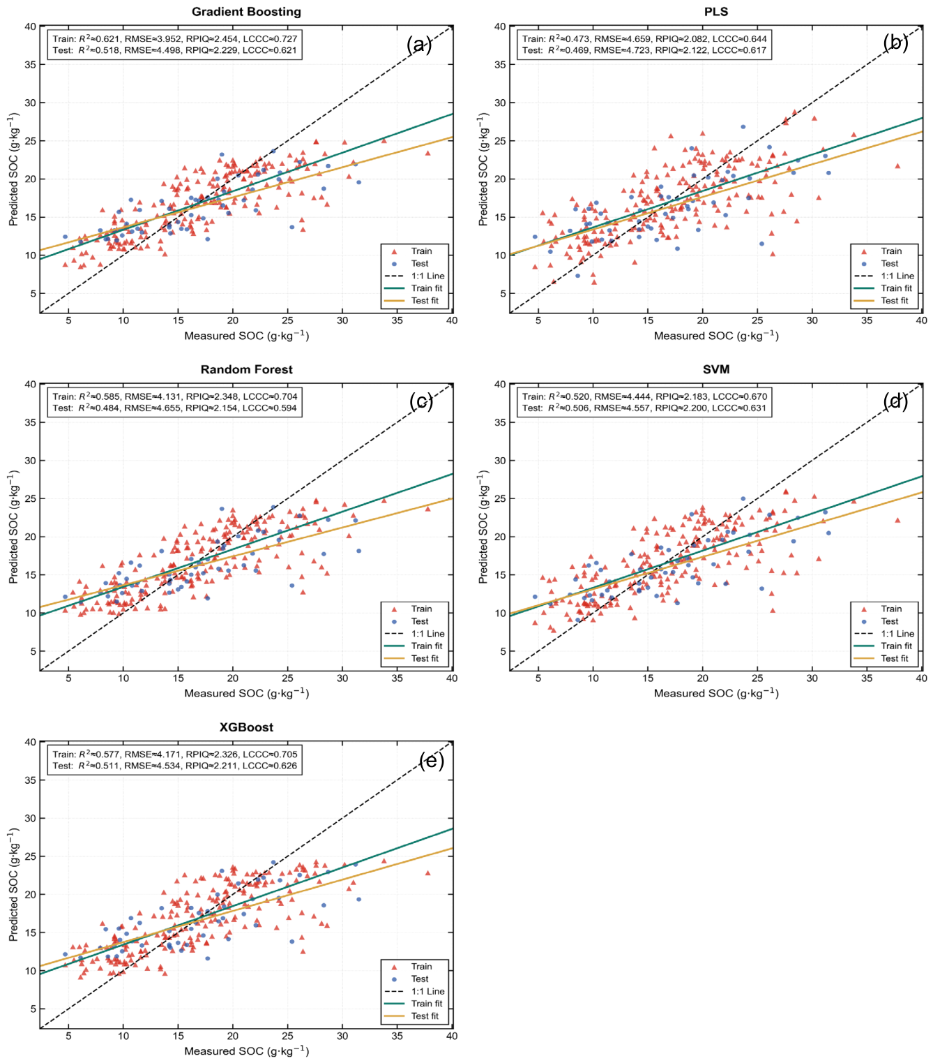
($R^2$, $\mathrm{RMSE}$, $\mathrm{MAE}$, $\mathrm{RPIQ}$, and $\mathrm{LCCC}$) were derived directly from these bias-corrected, back-transformed predictions. Table 3 summarizes the predictive performance of each model across both the training and independent test sets, whereas Figure 5 illustrates the correspondence between predicted and measured SOC values for the independent test set.

Among the five evaluated algorithms, gradient boosting decision trees (GBDT) consistently achieved the highest predictive accuracy on both the training and test sets. During the training phase, GBDT yielded the highest $R^2$ (0.660) and the lowest $\mathrm{RMSE}$ (3.952 $\mathrm{g}\cdot {\mathrm{kg}}^{-1}$), followed by random forest (RF; $R^2=0.585$) and XGBoost ($R^2=0.577$). Partial least squares (PLS) produced the lowest training performance ($R^2=0.442$). On the independent test set, GBDT again outperformed all other models, achieving the highest $R^2$ (0.518), the lowest $\mathrm{RMSE}$ (4.498 $\mathrm{g}\cdot {\mathrm{kg}}^{-1}$), the highest $\mathrm{RPIQ}$ (2.229), and an $\mathrm{LCCC}$ of 0.621 (Table 3). Support vector machine (SVM) attained a comparable $\mathrm{LCCC}$ (0.631) but exhibited lower overall predictive performance ($R^2=0.506$). XGBoost ($R^2=0.511$) and RF ($R^2=0.484$) showed intermediate performance, whereas PLS remained the least accurate ($R^2=0.469$). Visual analysis of the prediction scatter plots (Figure 5) corroborated these quantitative findings. GBDT predictions clustered most tightly along the 1:1 line, exhibiting minimal deviation across the entire SOC range. SVM displayed slight compression at the extremes, whereas RF and PLS showed greater dispersion, characterized by a systematic underestimation of values exceeding 30 $\mathrm{g}\cdot {\mathrm{kg}}^{-1}$. Based on its superior and consistent performance, GBDT was selected as the foundational architecture for final SOC mapping, SHAP-based feature interpretation, and uncertainty quantification.

To rigorously assess the spatial generalization capacity of the models, a spatial block cross-validation scheme was implemented. Consistent with expectations regarding spatial data leakage, all machine learning models exhibited a decline in predictive performance under spatial block cross-validation compared with conventional random cross-validation (

Table 4. Model performance comparison between random and spatial cross-validation schemes for SOC mapping.

Model	Random CV ${\mathit{R}}^2$	Spatial CV ${\mathit{R}}^2$	Random CV $\mathit{R}\mathit{M}\mathit{S}\mathit{E}$ ($\mathbf{g}·{\mathbf{k}\mathbf{g}}^{-1}$)	Spatial CV $\mathit{R}\mathit{M}\mathit{S}\mathit{E}$ ($\mathbf{g}·{\mathbf{k}\mathbf{g}}^{-1}$)
RF	0.410	0.369	4.940	5.105
GBDT	0.447	0.416	4.782	4.913
PLS	0.485	0.444	4.613	4.795
SVM	0.365	0.329	5.123	5.266
XGBOOST	0.348	0.321	5.192	5.298

). For the optimal gradient boosting decision tree (GBDT) model, the test $\mathrm{RMSE}$ increased from $4.498\mathrm{g}\cdot {\mathrm{kg}}^{-1}$ under random cross-validation to $4.913\mathrm{g}\cdot {\mathrm{kg}}^{-1}$ under spatial block validation, reinforcing the necessity of accounting for geographic heterogeneity when estimating model generalization. Nevertheless, our original stratified random validation scheme remains the most appropriate baseline for our final mapped products, as the quintile-based stratification successfully guaranteed distributional equivalence across all soil carbon tiers. Conversely, spatial block cross-validation functions as an overly pessimistic evaluation strategy given our limited sample size, where removing entire geographic clusters induces localized data scarcity and model underfitting rather than reflecting a true deficiency in model generalization capacity.

3.3. SHAP-Based Variable Importance and Response Patterns

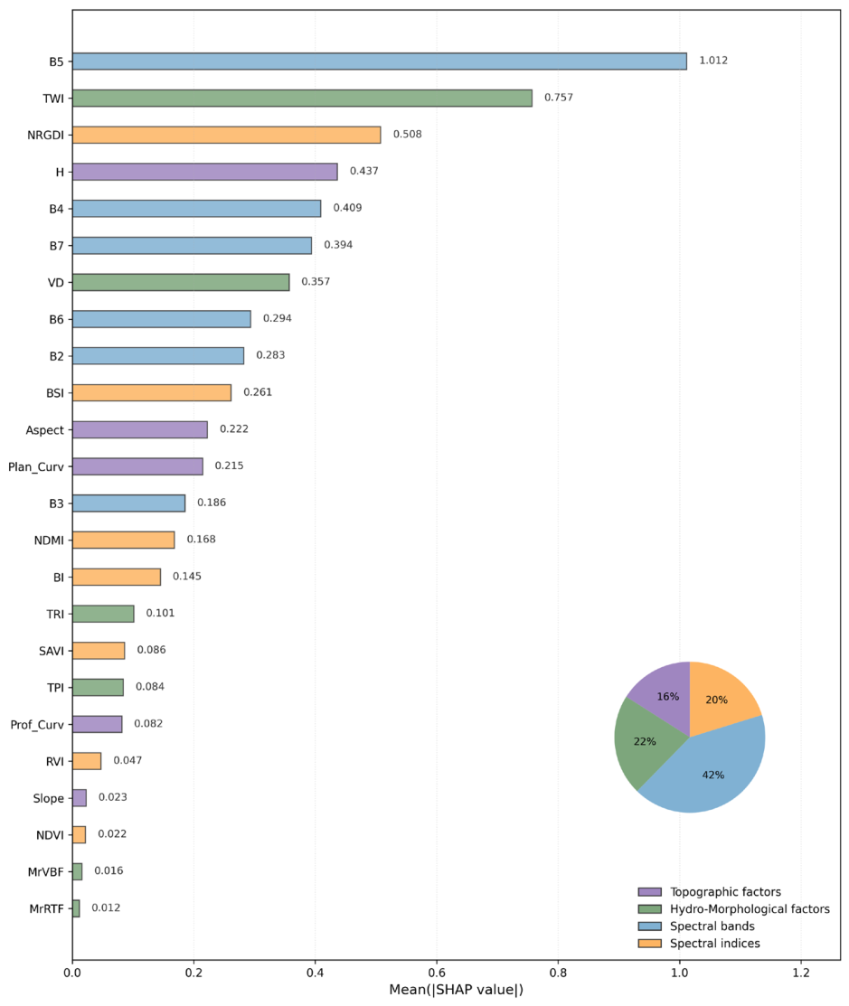
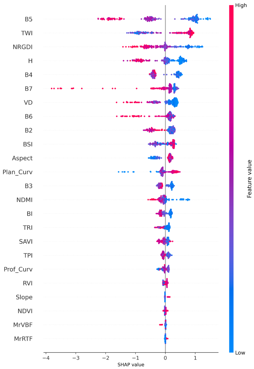
As indicated by the SHAP mean absolute value ranking (Figure 6), the near-infrared band (B5) emerged as the most influential predictor based on this metric, followed by the Topographic Wetness Index (TWI), Normalized Red–Green Difference Index (NRGDI), elevation (H), the red band (B4), and the SWIR2 band (B7). Collectively, spectral bands account for 42% of the total feature importance, suggesting that soil reflectance properties serve as the primary information source for soil organic carbon (SOC) estimation within this bare-soil composite dataset and model configuration. The SHAP summary plot (Figure 7) illustrates the directional relationship between predictor variables and SOC predictions: higher values of B5, NRGDI, H, B7, valley depth (VD), B6, B2, B4, and Normalized Difference Moisture Index (NDMI) correspond to lower predicted SOC (negative contribution), whereas higher values of TWI, the Bare Soil Index (BSI), and aspect correspond to higher predicted SOC (positive contribution).

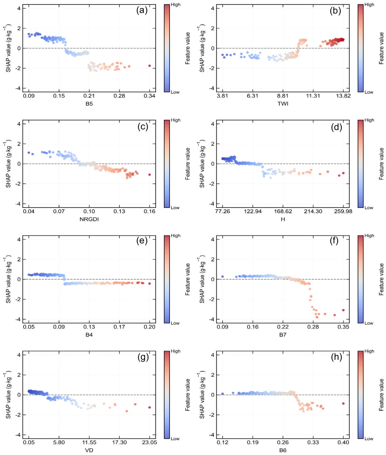
Figure 6 illustrates the global importance of environmental predictors derived from mean absolute SHAP values. Complementing this, the SHAP dependence plots in Figure 8 illustrate the nonlinear interactions between topographic and spectral covariates as captured by the model within the Hungarian study area. These patterns are consistent with a commonly observed inverse relationship: soil reflectance across the optical spectrum tends to decrease as soil organic carbon (SOC) content increases—a well-documented phenomenon in soil spectroscopy attributable to the chromophoric properties of organic matter.

The near-infrared band (B5; 0.85–0.88 $\mathsf{\mu }\mathrm{m}$) exerts a predominantly negative influence on SOC prediction, consistent with the aforementioned inverse reflectance–SOC relationship. The SHAP dependence plot (Figure 8a) suggests a model-inferred threshold near a reflectance value of approximately 0.16 within the Hungarian dataset; below this value, SHAP contributions are largely positive—signifying that low reflectance correlates with higher predicted SOC—whereas values exceeding this threshold correspond to negative contributions, potentially indicative of carbon-poor, mineral-dominated soils. Comparable transitions in SHAP contributions are observed for B4 (0.64–0.67 $\mathsf{\mu }\mathrm{m}$), B6 (1.57–1.65 $\mathsf{\mu }\mathrm{m}$), and B7 (2.11–2.29 $\mathsf{\mu }\mathrm{m}$).

Conversely, the Topographic Wetness Index (TWI) exhibits a consistently positive influence on SOC predictions. The SHAP dependence plot (Figure 8b) demonstrates a monotonic increase in SHAP values with rising TWI, transitioning from negative contributions at low values ($\mathrm{TWI}<3.9$) to strongly positive contributions in high-TWI regimes. This positive TWI–SOC correlation is spatially consistent with the results in Section 3.4, where high-SOC classes (IV and V) are predominantly localized in low-elevation alluvial depressions. Furthermore, spectral indices including the Normalized Red–Green Difference Index (NRGDI), Bare Soil Index (BSI), and Normalized Difference Moisture Index (NDMI) consistently exhibit negative SHAP contributions. In this context, NRGDI acts primarily as a proxy for soil brightness and iron content rather than as a vegetation discriminator; thus, higher values—associated with brighter, mineral-dominated surfaces—are inversely correlated with SOC, reinforcing the underlying spectral response patterns.

3.4. Spatial Prediction and Uncertainty Mapping

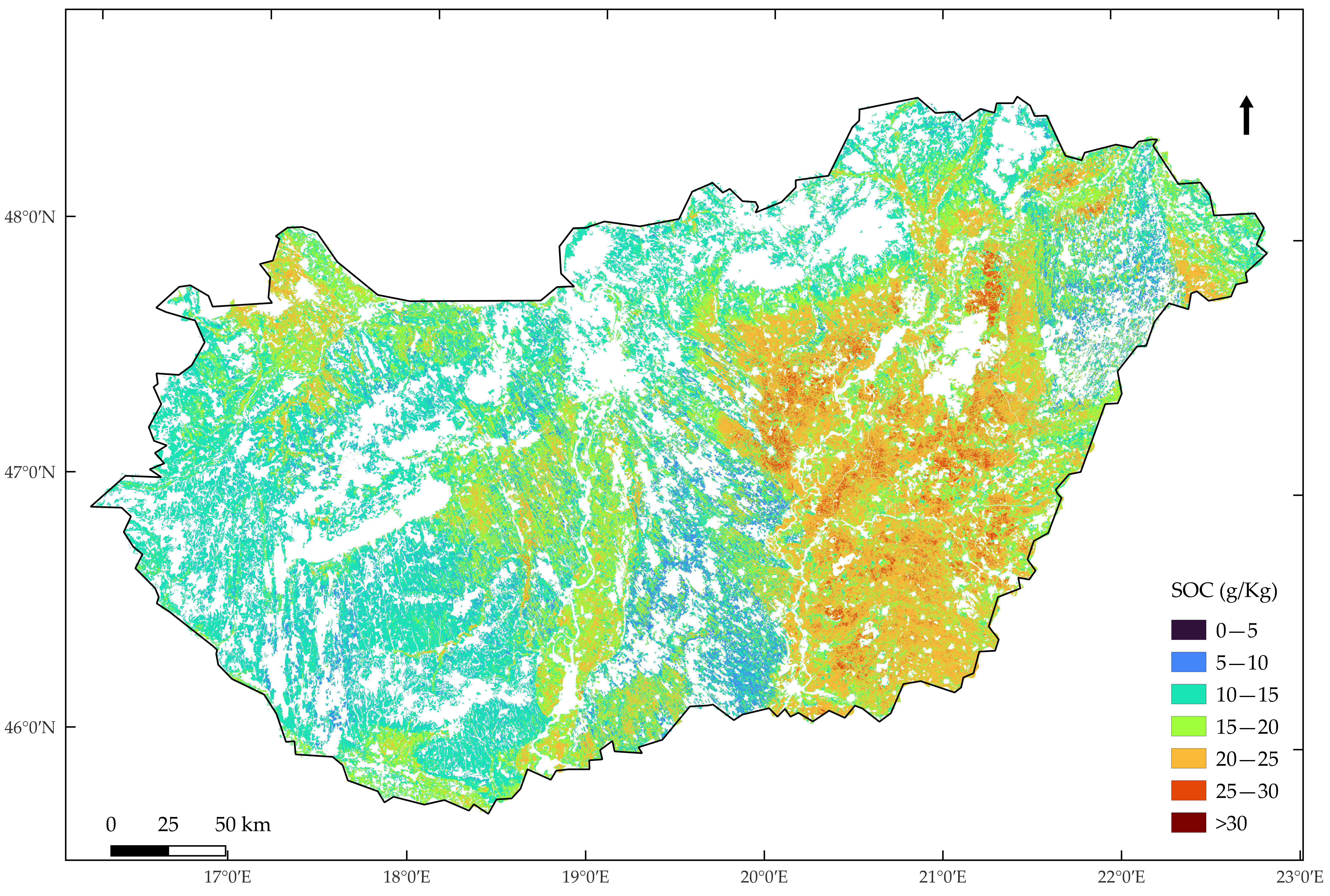
Utilizing the optimized gradient boosting decision tree (GBDT) model—which achieved a predictive performance of $R^2=0.518$ and $\mathrm{RMSE}=4.498\mathrm{g}\cdot {\mathrm{kg}}^{-1}$ under 10-fold cross-validation—a 30 m resolution map of topsoil soil organic carbon (SOC) was generated for the Hungarian cropland study area (Figure 9). The predicted SOC values ranged from 6.36 to 28.27 $\mathrm{g}\cdot {\mathrm{kg}}^{-1}$, with a mean concentration of $16.30\pm 4.65\mathrm{g}\cdot {\mathrm{kg}}^{-1}$. To facilitate the interpretation of spatial distribution patterns, these predictions were classified into five distinct tiers using 5 $\mathrm{g}\cdot {\mathrm{kg}}^{-1}$ intervals: Class I (5–10 $\mathrm{g}\cdot {\mathrm{kg}}^{-1}$), Class II (10–15 $\mathrm{g}\cdot {\mathrm{kg}}^{-1}$), Class III (15–20 $\mathrm{g}\cdot {\mathrm{kg}}^{-1}$), Class IV (20–25 $\mathrm{g}\cdot {\mathrm{kg}}^{-1}$), and Class V (25–30 $\mathrm{g}\cdot {\mathrm{kg}}^{-1}$).

To investigate topographic controls on soil carbon, five elevation zones were delineated from the digital elevation model (DEM) using natural breaks classification [44]. The distribution of SOC classes within these zones is detailed in

Table 5. Distribution of SOC content classes across different elevation zones.

Zone	Elevation Range (m)	Area (km2)	I (%)	II (%)	III (%)	IV (%)	V (%)
1	0–124	26,200.49	1179.02 (4.50)	3377.24 (12.89)	8143.11 (31.08)	12,319.47 (47.02)	1181.64 (4.51)
2	124–195	12,771.39	1325.67 (10.38)	6785.44 (53.13)	3731.80 (29.22)	927.20 (7.26)	1.28 (0.01)
3	195–305	3028.42	275.89 (9.11)	2386.70 (78.81)	356.75 (11.78)	9.09 (0.30)	0.00
4	305–482	192.96	24.33 (12.61)	161.30 (83.58)	7.31 (3.79)	0.04 (0.02)	0.00
5	>482	0.60	0.10 (16.94)	0.45 (74.06)	0.05 (9.00)	0.00	0.00

. Hungarian cropland is predominantly concentrated in the lowest elevation zone (0–124 m), which encompasses 62% of the total cropland area and contains the majority of high-SOC classes (IV and V; 51.5%). Conversely, Class II predominates in zones exceeding 124 m, accounting for 53–84% of the area in these elevated regions. While the proportion of high-SOC classes declines markedly with increasing elevation, Class I—observed in both sandy lowlands and high-altitude, cool uplands—characterizes the textural and erosional extremes of the SOC gradient.

The 30 m SOC map demonstrates a pronounced east–west zonation across Hungarian croplands: higher SOC concentrations are localized in the eastern and southeastern plains, whereas lower values prevail in western and hilly regions. Class II represents the largest areal extent, while Classes IV and V are largely restricted to low-elevation plains. Class I appears sporadically on aeolian sand dunes of the Great Plain and in high-elevation northern croplands; Class III extends across the central region toward the northern foothills and western borders; and Class V occurs as scattered patches within northeastern alluvial depressions and southern lowlands. These broad spatial patterns align with the Global Black Soil Map (GBSmap) [45] and the national-level product of Szatmári et al. [6].

Complementing this regional agreement, the 30 m resolution captures intra-class heterogeneity that coarser products fail to resolve. In the eastern high-SOC belt, contiguous Class IV patches are interspersed with localized Class V occurrences, while small Class I fragments delineate sandy dune landforms in the southern study area. This finer spatial resolution exposes local-scale SOC variations associated with soil type boundaries, microtopographic depressions, and isolated sand lenses—features inherently smoothed by coarser mapping products. Such granularity has direct implications for site-specific management, as it delineates zones of contrasting carbon status within fields that would otherwise be treated as spatially uniform.

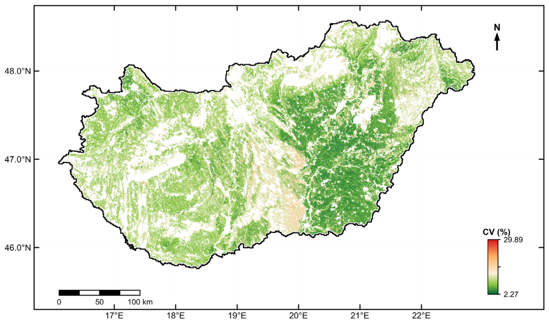
A pixel-level coefficient of variation ($\mathrm{CV}$) map, derived from 100 bootstrap resampling iterations, was generated to quantify the spatial distribution of SOC prediction uncertainty (Figure 10). The lowest uncertainty ($\mathrm{CV}<15\%$, dark green) is concentrated in the eastern Great Plain (46.8–47.3° N, 18.5–21.0° E), overlapping extensive high-SOC zones dominated by Chernozems. This correspondence between high prediction confidence and high SOC is attributable to the model’s reliance on the B5 band. In this region, the deep, dark humic horizons of Chernozems produce persistently low near-infrared (NIR) reflectance, providing a stable spectral signature for the model’s most influential predictor. Furthermore, the subdued topography and gradual soil transitions here reduce the complexity of predictor–response relationships, fostering greater prediction stability.

Conversely, higher uncertainty is concentrated in two primary zones. The first encompasses the southern Danube–Tisza interfluve and the Kiskunság sand region (~46.0° N), where sandy, coarse-textured soils dominate. Here, the fine-scale mosaic of aeolian sands and Chernozems induces high-frequency spatial variation that the current predictor set cannot fully resolve. The second zone lies in the western Transdanubian Hills (~17° E), where the landscape transitions from hills to plains and soil types shift abruptly from Cambisols to Fluvisols along valley axes. The intermingling of river terraces, floodplains, and hillslopes creates rapid successions of soil and topographic conditions, thereby elevating prediction uncertainty. Finally, the northern high-elevation region exhibits moderate uncertainty; despite the pronounced relief, regional-scale topographic proxies are insufficient to fully capture localized carbon enrichment within closed depressions of the Luvisol–Chernozem mosaic.

To evaluate the calibration of the bootstrap-derived prediction intervals, the Prediction Interval Coverage Probability (PICP) and Mean Prediction Interval Width (MPIW) were assessed at the 95% confidence level on the independent test set. The PICP was 94.59%, and the MPIW was 13.65 $\mathrm{g}\cdot {\mathrm{kg}}^{-1}$.

To assess whether significant spatially structured processes remained unaccounted for, the spatial autocorrelation of prediction residuals from the optimal GBDT model was analyzed using global Moran’s $I$. Three $k$-nearest neighbor (KNN) spatial weight matrices were evaluated ($k=5,7,10$). The resulting global Moran’s $I$ values were $-0.0175$ ($p=0.832$), $0.0001$ ($p=0.999$), and $0.0154$ ($p=0.795$), calculated via 9999 randomized Monte Carlo permutations. The lack of statistically significant spatial autocorrelation in the residuals suggests that the model successfully captured the spatial dependencies inherent in the SOC data. Furthermore, a control experiment was conducted to determine if incorporating macro-scale covariates (mean annual temperature, mean annual precipitation, and categorical parent material) would enhance model accuracy. This inclusion failed to improve performance; the expanded GBDT model achieved a test $R^2$ of 0.476 (

Table 6. Model training and testing performance under the expanded covariate dataset.

Model	Dataset	${\mathit{R}}^2$	$\mathit{R}\mathit{M}\mathit{S}\mathit{E}$ ($\mathbf{g}·{\mathbf{k}\mathbf{g}}^{-1}$)	$\mathit{M}\mathit{A}\mathit{E}$ ($\mathbf{g}·{\mathbf{k}\mathbf{g}}^{-1}$)	$\mathit{R}\mathit{P}\mathit{I}\mathit{Q}$	$\mathit{L}\mathit{C}\mathit{C}\mathit{C}$
RF	Training	0.595	4.083	3.144	2.376	0.713
	Testing	0.469	4.725	3.701	2.122	0.595
GBDT	Training	0.577	3.952	3.048	2.454	0.727
	Testing	0.476	4.691	3.729	2.137	0.597
PLS	Training	0.506	4.509	3.486	2.151	0.677
	Testing	0.475	4.695	3.736	2.135	0.630
SVM	Training	0.463	4.701	3.656	2.064	0.614
	Testing	0.468	4.729	3.730	2.120	0.594
XGBOOST	Training	0.561	4.251	3.265	2.282	0.614
	Testing	0.511	4.713	3.656	2.127	0.600

). These findings suggest that the information dilution and spatial mismatch associated with integrating these macro-scale features outweighed their theoretical relevance when modeled at a 30 m resolution.

3.5. Temporal Window and Data Density Analysis

Beyond covariate selection, the temporal misalignment between ground-truth soil sampling and satellite acquisition periods constitutes a significant source of model uncertainty. To quantify the impact of this 1–5 year discrepancy—specifically the lag between the 2015 LUCAS sampling campaign and the 2016–2020 imagery framework—a temporal control experiment was conducted. An alternative multi-temporal bare-soil composite was reconstructed using Landsat 8 observations constrained to the sampling baseline (2013–2018). All five machine learning models were subsequently retrained and validated using identical spatial partitions, with comparative performance metrics on the independent test set summarized in

Table 7. Test performance metrics of the five machine learning models under the alternative temporal window composite (2013–2018).

Model	Dataset	${\mathit{R}}^2$	$\mathit{R}\mathit{M}\mathit{S}\mathit{E}$ ($\mathbf{g}·{\mathbf{k}\mathbf{g}}^{-1}$)	$\mathit{M}\mathit{A}\mathit{E}$ ($\mathbf{g}·{\mathbf{k}\mathbf{g}}^{-1}$)	$\mathit{R}\mathit{P}\mathit{I}\mathit{Q}$	$\mathit{L}\mathit{C}\mathit{C}\mathit{C}$
RF	Training	0.516	3.9287	3.617	2.843	0.684
	Testing	0.408	4.904	3.825	1.883	0.568
GBDT	Training	0.542	3.559	3.349	2.811	0.797
	Testing	0.412	4.885	3.774	1.884	0.585
PLS	Training	0.502	4.539	3.520	2.148	0.669
	Testing	0.421	4.855	3.864	1.893	0.620
SVM	Training	0.494	4.575	3.463	2.131	0.638
	Testing	0.407	4.916	3.869	1.877	0.569
XGBOOST	Training	0.500	4.376	3.274	2.391	0.767
	Testing	0.373	5.041	3.939	1.824	0.584

. Restricting imagery to the 2013–2018 window uniformly degraded performance across all algorithms, indicating that observation density outweighed strict temporal proximity for this multi-temporal composite.

3.6. Comparative Assessment with Existing SOC Products

Table 8. Statistical comparison between our prediction and three benchmark SOC products.

Product	Depth	Mean (g kg−1)	Std (g kg−1)	Pearson r	RMSE (g kg−1)	Bias (g kg−1)	LCCC	Slope	Intercept
Our study	0–20	17.42	4.85	-	-	-	-	-	-
SERENA 2016	0–30	13.04	3.64	0.616	5.86	+4.37	0.388	0.83	+6.64
SoilGrids 2.0	0–30	18.75	2.19	0.416	4.61	−1.35	0.294	0.94	−0.11
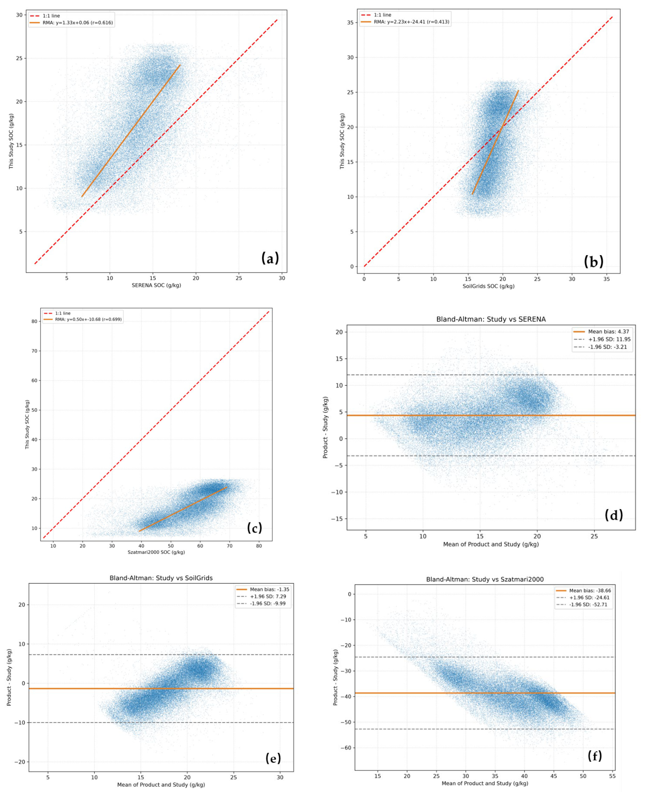
Szatmári 2000	0–30	56.07	9.70	0.699	39.31	−38.66	0.041	0.35	−2.27

summarizes the statistical comparison between our GBDT-derived SOC prediction (0–20 cm) and the three benchmark products (all 0–30 cm). Our map demonstrated Pearson correlations ($r$) of $r=0.616$ with SERENA 2016, $r=0.416$ with SoilGrids 2.0, and $r=0.699$ with Szatmári 2000. The respective biases relative to these benchmarks were $+4.37$, $-1.35$, and $-38.66\mathrm{g}\cdot {\mathrm{kg}}^{-1}$. In terms of Lin’s concordance correlation coefficient ($\mathrm{LCCC}$), SERENA 2016 achieved the highest agreement ($\mathrm{LCCC}=0.388$), whereas Szatmári 2000 displayed minimal concordance ($\mathrm{LCCC}=0.041$). Although SoilGrids 2.0 yielded the lowest $\mathrm{RMSE}$ ($4.61\mathrm{g}\cdot {\mathrm{kg}}^{-1}$) and bias ($-1.35\mathrm{g}\cdot {\mathrm{kg}}^{-1}$), it exhibited the weakest correlation and a standard deviation of $2.19\mathrm{g}\cdot {\mathrm{kg}}^{-1}$—representing only 45% of the spatial variability captured by our map—suggesting an underestimation of spatial heterogeneity. Reduced Major Axis (RMA) regression slopes for SERENA, SoilGrids 2.0, and Szatmári 2000 were 0.83, 0.94, and 0.35, respectively (Table 8; Figure 11a–c). The Bland–Altman analysis yielded 95% limits of agreement of [$-3.21,11.95$] $\mathrm{g}\cdot {\mathrm{kg}}^{-1}$ for SERENA (characterized by a funnel-shaped distribution), [$-9.99,7.29$] $\mathrm{g}\cdot {\mathrm{kg}}^{-1}$ for SoilGrids 2.0 (the narrowest range), and [$-52.71,-24.61$] $\mathrm{g}\cdot {\mathrm{kg}}^{-1}$ for Szatmári 2000. The latter benchmark’s limits, being entirely negative, indicate a systematic and substantial underestimation of SOC content across the study area.

Pixel-wise difference maps (Figure 11d–f) revealed distinct spatial structures in the predictive bias relative to the benchmark products. Comparisons with SERENA 2016 indicated a clear spatial gradient, characterized by positive bias in the eastern Great Plain and negative bias in the western hilly and southern sandy regions. Conversely, residuals relative to SoilGrids 2.0 were centered near zero, with deviations limited to localized discrepancies in sandy zones. Finally, the comparison with the Szatmári 2000product demonstrated a pronounced, systematic negative bias across the entire study area.

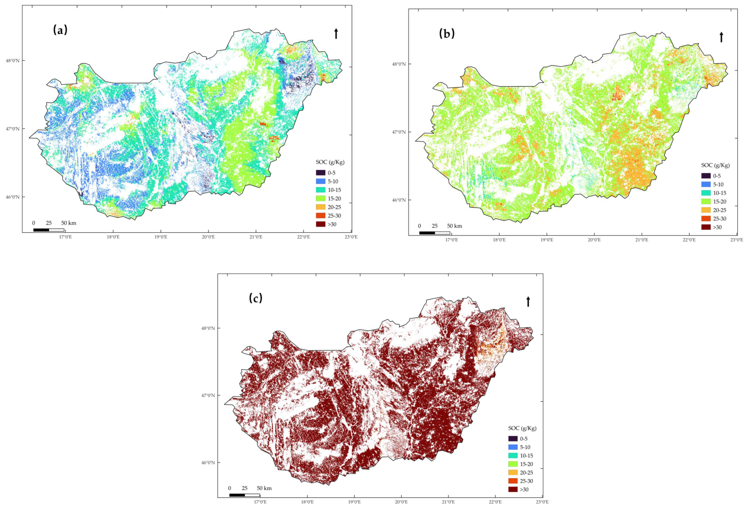
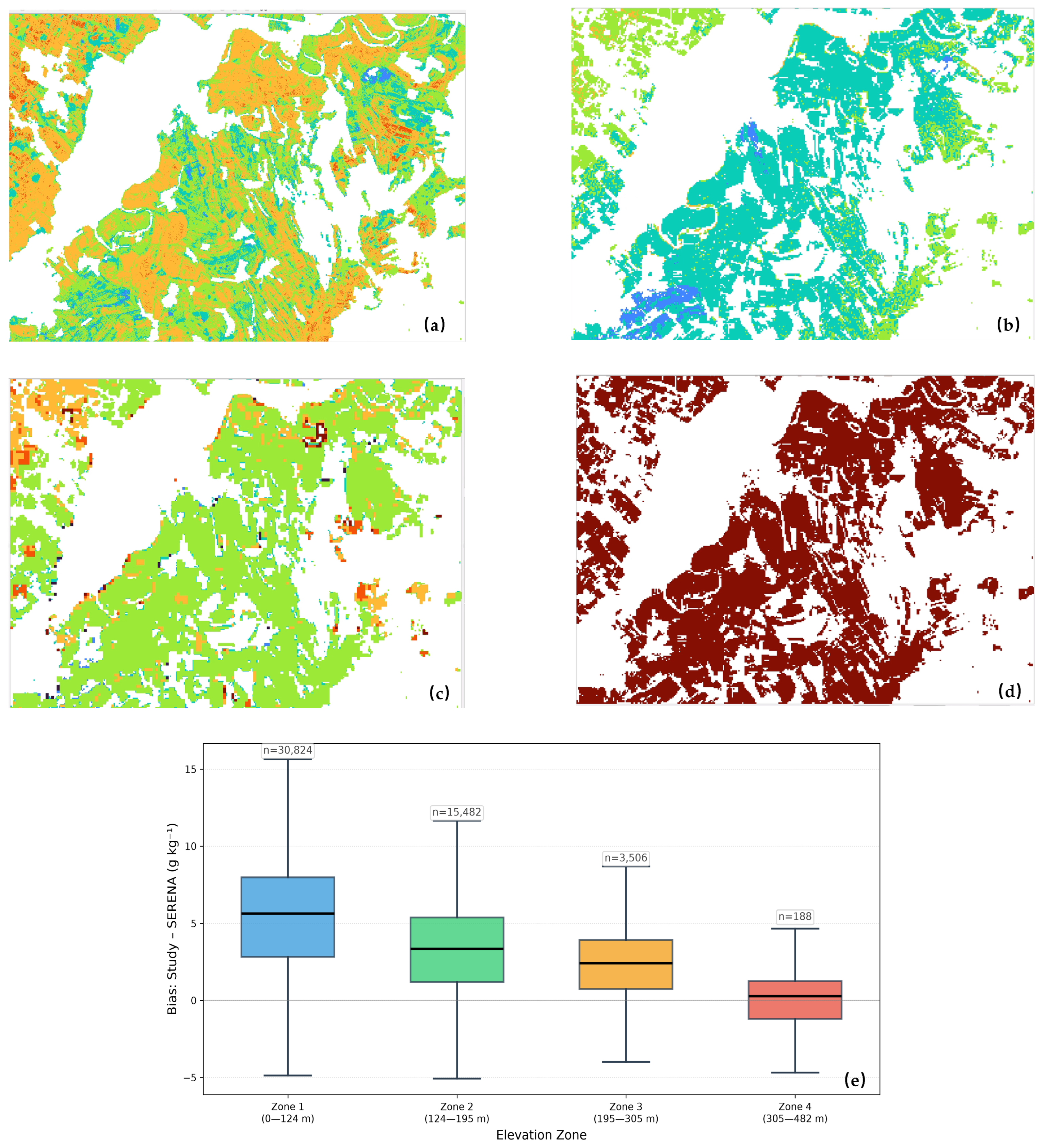
A comparative visual analysis between our 30 m SOC map (Figure 9) and the three benchmark products (Figure 3) reveals that our results provide the most refined delineation of the east–west SOC zonation, characterized by distinct spatial boundaries. While the SERENA product successfully reproduces macro-scale patterns, it exhibits noticeable smoothing at transition zones. SoilGrids 2.0 presents a comparatively homogenized landscape, likely attributable to resolution-induced aggregation. Although the Szatmári 2000 product demonstrates high spatial similarity ($r=0.700$), it consistently reports higher absolute SOC magnitudes across the study area. Detailed inspection of local subsets (Figure 12a–d) confirms that our 30 m map captures sharper SOC gradients at finer spatial scales, whereas the 100 m and 250 m products progressively attenuate these transitions, effectively masking local-scale pedological heterogeneity.

Using the SERENA product as a reference, we assessed the spatial structure of the difference raster using a spatial clustering index ($I=0.456\pm 0.007,p<0.01$), which confirmed a statistically significant spatial clustering of the prediction bias ($p<0.001$). The focal Pearson correlation analysis, computed within $5\times 5$ pixel windows, yielded a median $r=0.010$; however, this aggregate value masked considerable local heterogeneity, as 21.9% of locations exhibited negligible correlations ($\left|r\right|<0.1$), whereas 13.6% demonstrated strong local correlations ($r>0.5$). Furthermore, the bias relative to SERENA exhibited a significant negative correlation with elevation ($r=-0.3325,p<0.0001$). A zonal analysis across five elevation strata revealed a monotonic trend, with mean bias decreasing from $+5.22\mathrm{g}\cdot {\mathrm{kg}}^{-1}$ in the lowest elevation zone (Zone 1: 0–124 m) to $-2.44 \mathrm{g}\cdot {\mathrm{kg}}^{-1}$ in the highest zone (Zone 5: $>482 \mathrm{m}$) (

Table 9. Bias (study−SERENA) across five elevation zones.

Zone	Elevation (m)	Valid Pixels	Proportion	Mean Bias (g kg−1)	Median	Q1	Q3
1	0–124	25,271,782	61.8%	+5.22	+5.66	+2.82	+8.00
2	124–195	12,628,779	30.9%	+3.27	+3.37	+1.22	+5.37
3	195–305	2,857,001	7.0%	+2.18	+2.41	+0.67	+3.92
4	305–482	157,331	0.4%	+0.05	+0.16	−1.15	+1.42
5	>482	119	<0.01%	−2.44	−1.64	−4.28	−0.67

, Figure 12e). All subsample-based bootstrap validations demonstrated high stability, with coefficient of variation ($\mathrm{CV}$) values $<2\%$.

4. Discussion

4.1. Comparative Evaluation of Machine Learning Algorithms

The performance hierarchy observed—GBDT > SVM > XGBoost > RF > PLS—reflects the interplay among three factors: the heterogeneous environmental conditions across Hungarian croplands, the architectural logic of each algorithm, and the statistical distribution of the SOC dataset. The study area is a complex mosaic: fertile Chernozems and meadow soils dominate the plains, while Luvisols and Cambisols characterize the surrounding hilly and mountainous regions. This spatial structuring, coupled with the skewed SOC distribution, necessitates models capable of capturing strongly nonlinear predictor–response relationships. Boosting models demonstrated a distinct advantage in this context. The GBDT model, through sequential residual fitting, adaptively isolates and reduces bias in the most complex regions of the predictor space. The high concordance of its predictions around the $1:1$ identity line, particularly at high SOC values, confirms its efficacy in resolving local nonlinearities. Although XGBoost is based on similar principles, it consistently performed marginally lower than GBDT. XGBoost incorporates $L_1$ and $L_2$ regularization alongside more aggressive tree-pruning strategies, which, while robust, may overly constrain the model when mapping sharp SOC transitions relative to soil type and topographic position. Given the training dataset size ($N=259$), the bias incurred by these regularization constraints appears to exceed the corresponding gain in variance reduction, resulting in the observed performance gap.

The performance of RF reinforces the importance of bias correction. Bagging suppresses variance by averaging predictions over decorrelated trees but lacks an intrinsic mechanism to correct for bias in highly nonlinear feature spaces. Consequently, RF predictions gravitate toward the global mean, systematically overestimating low-SOC sites and underpredicting high-SOC values (Figure 3c). The lower Lin’s concordance correlation coefficient ($\mathrm{LCCC}=0.594$) compared to boosting models suggests that bias, rather than variance, is the dominant limitation for RF in this application. Conversely, SVM excelled in systematic error suppression, achieving the highest $\mathrm{LCCC}$ ($0.631$) despite a marginally lower $R^2$ than GBDT. This performance is attributable to its $ϵ$-insensitive loss function and the structural risk minimization principle, which balance model complexity against empirical risk. While this design slightly compresses the predicted range—curtailing extreme output, it minimizes large systematic residuals. For practical applications, this implies a bias–variance trade-off: SVM may be preferable for national-scale carbon stock assessments where systematic bias reduction is critical, whereas GBDT is better suited for applications prioritizing localized predictive precision. Finally, the inferiority of PLS confirms that linear latent-variable formulations are inadequate for capturing the complex, nonlinear associations present in hyperspectral SOC data, as evidenced by its severe underestimation at high SOC levels.

While the optimized GBDT model achieved moderate accuracy ($R^2=0.518$, $\mathrm{RMSE}=4.498 \mathrm{g}\cdot {\mathrm{kg}}^{-1}$), this performance is consistent with regional-scale digital soil mapping (DSM) benchmarks. Previous assessments across Latin America and national-scale mapping in Hungary by Szatmári et al. [6] reported cross-validated $R^2$ values between $0.39$ and $0.42$. Our higher-resolution ($30 \mathrm{m}$) model achieves competitive performance despite a more limited sample size, suggesting that the integration of localized spectral proxies helps mitigate the effect of limited sample size. However, given the moderate predictive accuracy, these results should be interpreted as regional spatial trends rather than exact field-scale metrics. Following the D1–D5 resolution framework [46], our $30 \mathrm{m}$ resolution corresponds to the D3 category (20–200 m), which is intended for catchment-to-regional applications such as carbon auditing or conservation targeting, rather than sub-hectare precision management. The accompanying pixel-wise uncertainty map remains critical for operational use, signaling where predictions are robust and where supplementary sampling is required. Ultimately, this investigation illustrates the “no free lunch” principle in DSM: model selection must be driven by local benchmarking and data characteristics rather than a priori preference.

4.2. Interpretation of Nonlinear Covariate Effects

The SHAP dependence plots (Section 3.3) reveal two primary mechanistic insights. The first offers a plausible interpretation of model behavior, suggesting an optical absorption–scattering transition inferred from the B5 reflectance threshold near 0.16. One interpretation is that at reflectance values below this threshold, absorption by organic matter suppresses the near-infrared (NIR) signal, whereas above it, the spectral response could be more strongly influenced by mineral components characterized by inherently higher reflectance. However, this threshold is derived from the specific model and dataset used here and should not be treated as a universal spectroscopic constant. The second insight relates to the behavior of spectral indices under the bare-soil compositing protocol. Because this compositing approach selects the driest, most exposed pixel state and minimizes vegetation contamination, the Normalized Difference Moisture Index (NDMI) no longer functions as a traditional moisture indicator. Instead, high NDMI values serve as a proxy for bright mineral surfaces—such as aeolian sands and loess-derived soils—that are inherently low in organic matter and facilitate strong mineral scattering.

These dependency patterns confirm that the relationship between SOC and key environmental predictors is inherently nonlinear, with many spectral and topographic variables exerting influence through abrupt transitions rather than steady, linear gradients. This prevalence of nonlinear structure explains the observed performance hierarchy: the classical GBDT model, with minimal regularization, closely tracks these sharp threshold breaks without incurring penalties for model complexity, thereby systematically outperforming the more constrained XGBoost and linear alternatives. These reflectance transition zones also possess practical value for field applications. Under bare-soil conditions, a spectral domain defined by B5 reflectance values ($\mathrm{B}5<0.16$) enables direct flagging of potentially high-SOC cropland from remote sensing imagery—a simple screening procedure to guide targeted soil sampling and prioritize conservation tillage zones [46]. However, it must be emphasized that these transition values represent model-specific associations derived from the Hungarian training data, rather than universal spectroscopic thresholds; their transferability to other regions requires independent validation using local soil spectral libraries.

The consistently positive TWI–SOC association warrants mechanistic interpretation grounded in landscape evolution. This association aligns with the framework established by Moore et al. [47], who posit that the wetness index serves as a proxy for A-horizon thickness and organic matter accumulation, interpreting the A-horizon as a “fossil record” of terrain-controlled sediment redistribution. This interpretation is corroborated by broad empirical evidence: Wiesmeier et al. [48] identified TWI as the primary driver of SOC storage across 384 Bavarian cropland profiles ($\beta =0.38-0.42$); Zádorová et al. [49] demonstrated that TWI effectively delineates colluvial soils where SOC accumulates in concave positions; and Li et al. [50] found TWI to be the most influential control on SOC density ($r=0.735,P<0.0001$) across 560 U.S. Corn Belt sites. Collectively, these findings indicate that the positive TWI–SOC correlation in croplands primarily reflects long-term topographic controls on organic matter accumulation, rather than instantaneous moisture status. In Hungarian croplands—where artificial drainage and tillage override natural hydrological patterns—this represents a depositional legacy effect, wherein high TWI values identify landscape positions that historically functioned as sinks for eroded, organic-rich topsoil. Consistent with this, our SHAP analysis identifies a model-inferred transition from negative to positive contributions at a TWI value of 3.9. This value serves as a data-driven reference point specific to the Hungarian cropland dataset rather than a universally applicable geomorphic threshold.

Despite the robustness of these findings, two primary limitations should be noted. First, in the absence of in situ measurements of soil redox potential, microbial activity, or long-term hydrological monitoring, our “legacy interpretation” remains partially inferential. Definitive disentanglement of historical sediment accretion versus modern moisture regime contributions would require complementary datasets. Second, the SHAP-derived thresholds are specific to the Hungarian context and may not directly transfer to regions with distinct soil types, climate regimes, or land management histories. Future work should investigate the generalizability of these thresholds across broader agroecological settings.

4.3. Environmental Controls on SOC Spatial Heterogeneity

The observed nonlinear covariate effects (Section 3.3) manifest spatially as distinct SOC distribution patterns across Hungary’s altitudinal gradient. Class V is almost entirely restricted to the lowest elevation zone (Zone 1), with its spatial footprint—along with that of Class IV—narrowing progressively as elevation increases. This sequential contraction suggests that the highest carbon stocks are inextricably linked to flat, low-relief terrain, a pattern consistent with observations in temperate mountain regions [37]. However, within the study area, this elevational signal reflects more than simple climatic control; it is fundamentally mediated by the distribution of parent materials and depositional landforms. Fertile alluvial depressions and Chernozem-mantled plains are concentrated in these low-lying zones, where thick organic horizons have developed from base-rich parent materials, sustained by long-term sediment accretion and agricultural enrichment. Conversely, at higher elevations in the Transdanubian Hills, Luvisols and Cambisols become dominant. Here, moderate organic inputs coupled with accelerated decomposition kinetics maintain Class II as the prevalent SOC category.

Class I emerges in two distinct pedological niches. Across the cool, humid northern uplands, steep slopes undergo accelerated erosion that strips fertile topsoil; the resulting loss of soil volume and nutrients restricts root-zone organic inputs, overriding any potential carbon sequestration benefits of slower decomposition. In the lowland sandy tracts, rapid drainage, low cation exchange capacity, and minimal mineral protection act in concert to suppress organic matter retention. These divergent settings illustrate that SOC is not governed by elevation per se but rather covaries with an ensemble of soil-forming factors. The spatial agreement of our map with the Global Black Soil Map (GBSmap) [45] and the product of Szatmári et al. [6] confirms that our model accurately captures these regional patterns associated with Chernozems, the primary high-SOC soil type in Hungarian croplands.

The spatial configuration of SOC across the study area is governed by the interplay of topography, soil type, and land use. In the northern mountains, Luvisol–Chernozem landscapes are interspersed with closed depressions; these topographic lows act as local sinks, intercepting and retaining sediment and runoff from adjacent slopes. Such inputs sustain localized carbon enrichment that would otherwise be absent. A different spatial dynamic characterizes the eastern Great Plain, where extensive Chernozems with deep, dark humic horizons reflect historically robust carbon accumulation. Model predictions confirm the prevalence of contiguous Class IV and Class V cover, consistent with the high baseline fertility of these soils. Nevertheless, intensive long-term cultivation has likely diminished the original carbon stock, as repeated mechanical tillage and reduced residue inputs accelerate SOC mineralization. High-SOC patches persist primarily within alluvial depressions, where higher moisture availability and finer sediment fractions retard decomposition, providing a measure of protection for Class V SOC [39]. The cultivation imprint is further modulated in the Danube–Tisza interfluve, where a fine-scale mosaic of aeolian sands and Chernozems imposes edaphic heterogeneity, resulting in high local SOC variability [39]. In the Kiskunság sand region, sandy, coarse-textured soils dominate. Biomass production is restricted by low water-holding capacity, and organic matter decomposition is heightened; consequently, the decline to Class I on marginal dunes represents an extreme expression of this textural constraint [40]. Finally, the western Transdanubian Hills are defined by rapid transitions from Cambisols to Fluvisols along valley axes. The intimate juxtaposition of Class II and Class III reflects the complex patchwork of weakly developed alluvial soils and colluvial material from adjacent slopes. The carbon stored here is relatively labile; the geologically young alluvial deposits and coarse-textured Fluvisols offer limited capacity for organic matter stabilization. Across these environments, macro-scale SOC patterns are shaped by fundamental soil–geomorphology interactions. These interactions establish a physical template upon which secondary processes—hydrological redistribution, cultivation history, and microtopography—exert their influence [51]. The relative importance of these controls varies geographically: cultivation acts as a primary modifier in the eastern plains, soil texture and drainage dominate in the south, and alluvial dynamics drive soil carbon variability in the west.

4.4. Uncertainty Sources, Residual Diagnostics, and Model Constraints

The discrepancy in model performance between conventional random cross-validation and spatial block cross-validation highlights the confounding effect of spatial autocorrelation in digital soil mapping. Random validation strategies often suffer from optimistic bias, as nearby training and testing points share redundant environmental footprints. By applying geographically isolated validation blocks, we effectively broke this spatial dependency. The performance decay observed in our GBDT framework under spatial block cross-validation ($R^2$ decreasing to 0.416) unmasks the accuracy inflation inherent in conventional random validation. While this confirms that our model relies on deterministic soil–environmental relationships rather than localized spatial interpolation artifacts, it also underscores that model performance remains moderate and geographically bounded.

The absence of residual spatial structure (global Moran’s $I=-0.0175$, $p>0.05$; Section 3.4) indicates that our integration of multi-temporal Landsat bare-soil composites and microtopographic DEM derivatives successfully exhausted the deterministic, spatially structured environmental variance of topsoil SOC. The degradation in performance observed in our macro-covariate control experiment ($R^2$ dropping to 0.476; Table 6) further clarifies the constraints of incorporating broader climatic factors. This is primarily governed by scale mismatch and information dilution. While our objective centers on 30 m field-scale mapping to capture sharp spatial heterogeneities, coarse climate grids (~1 km) and generalized parent material polygons introduce significant spatial smoothing. When resampled to a 30 m grid, these uniform pixel blocks act as structural noise in tree-based splitting algorithms, diluting fine-scale topographic and spectral signals. Moreover, within the relatively homogeneous macro-climatic baseline of Hungarian agricultural zones, microtopography (governing soil redistribution and hydrology) and surface management are the dominant drivers of SOC variance. Consequently, the remaining unexplained variance (~48%) in our optimal GBDT framework is not an artifact of omitted natural environmental controls, but it is instead strongly modulated by highly fragmented, localized, and stochastic anthropogenic management—such as specific crop rotations, variable organic fertilization, and distinct tillage regimes. We acknowledge that this interpretation remains inferential, as direct management data were unavailable. Critically, these practices operate at sub-field scales and remain largely invisible to current satellite-based optical sensors, representing an inherent boundary of spectral–temporal remote sensing. This finding does not indicate a framework deficiency but rather underscores that field-scale SOC prediction requires region-specific calibration using locally relevant predictors.

We also assessed the impact of the temporal lag between the 2015 LUCAS sampling campaign and the 2016–2020 Landsat predictor window. While theoretical concerns regarding non-synchronous datasets exist, topsoil SOC is a relatively conservative property characterized by slow change vectors. Our control experiment, which reconstructed a bare-soil composite strictly surrounding the sampling baseline (2013–2018) [52], showed inferior performance (GBDT $R^2$ dropped from 0.518 to 0.412; Table 7). This highlights that observation density and sensor consistency heavily outweigh strict temporal proximity in multi-temporal bare-soil mapping. The 2016–2020 window contained a significantly larger volume of high-quality, cloud-free scenes, resulting in a statistically superior surface composite that bolstered predictive stability.

The spatial pattern of uncertainty reflects the alignment between environmental predictors and SOC heterogeneity. In regions with uniform terrain, the stable signal of the dominant spectral predictor ensures high confidence. Conversely, where soils form fine-scale mosaics, the predictor suite is less capable of resolving high-frequency variation, leading to elevated uncertainty. Our bootstrap-based framework addresses the research gap regarding the under-prioritization of uncertainty assessment in machine learning-based soil studies [46]. To verify that these bootstrap estimates reflect actual prediction reliability, we evaluated interval-based validation metrics. The framework yielded a Prediction Interval Coverage Probability (PICP) of 94.59%, highly consistent with the theoretical 95% confidence threshold, with a Mean Prediction Interval Width (MPIW) of 13.65 $\mathrm{g}\cdot {\mathrm{kg}}^{-1}$. These results indicate that the estimated intervals effectively encompass observed SOC variations. This “prediction plus confidence” dual-layer framework offers a distinct advantage over single-product outputs: it equips users with spatially explicit reliability. In low-uncertainty zones (e.g., eastern Great Plain), SOC predictions can support macro-scale nutrient budgeting. In high-uncertainty zones, the confidence layer explicitly prioritizes supplementary field sampling or conservative management, providing a risk-aware baseline for landscape-level conservation goals.

4.5. Implications of the Comparative Assessment with Existing SOC Products

The primary factor influencing numerical comparisons between our 0–20 cm GBDT map and existing 0–30 cm benchmarks is the vertical stratification of soil organic carbon (SOC). As organic carbon concentrations typically exhibit an exponential decay with depth [37], and considering that the 0–20 cm layer accounts for approximately 70–85% of total stock within the 0–30 cm profile, our map naturally tends toward higher absolute values. The positive bias observed against SERENA 2016 is consistent with this expectation. Therefore, all numerical discrepancies reported herein must be interpreted with this depth-dependent vertical stratification in mind.

The moderate macro-scale correlation with SERENA suggests that our 30 m GBDT model, despite being trained on a restricted sample size ($N=1528$), captures the dominant SOC zonation established by the national-scale SIMS-based product (~9385 observations). While global trends remain consistent—demonstrated by the high-SOC plains in the eastern Great Plain and the low-SOC western hills—our focal correlation analysis reveals a striking local-scale divergence. The near-zero median focal correlation indicates that while both products track broad climatic and pedological gradients, they capture fundamentally different spatial structures at the sub-field scale. Our 30 m framework preserves soil-type boundaries, microtopographic depressions, and localized sand lenses that the 100 m SERENA product systematically smooths. The spatial clustering of bias, modulated by elevation, further confirms that these discrepancies are driven by the vertical stratification effect: in low-elevation plains where SOC is highest, the “dilution” of the 0–30 cm mean by the deeper, lower-carbon 20–30 cm layer is most pronounced, resulting in larger positive bias in our product. SoilGrids 2.0 provides the closest numerical agreement in central tendency; however, its lower correlation and standard deviation expose a fundamental trade-off: global coarse-resolution products often prioritize mean value accuracy at the expense of spatial variability. This aligns with recent findings indicating that global soil maps often suffer from sparse local sampling and outdated legacy data, limiting their utility for field-level decision-making. The substantially lower spatial variance in SoilGrids relative to our map suggests that 250 m resolution is insufficient to resolve the field-scale heterogeneity critical for precision agriculture. The near-unity Reduced Major Axis (RMA) slope against SoilGrids suggests that while spatial correlation is weak, the products exhibit minimal systematic scale-dependent bias, illustrating that low $\mathrm{RMSE}$ does not guarantee spatial congruence—smoothing effects can decouple aggregate error metrics from spatial accuracy.

The high correlation with Szatmári et al. (2000) is consistent with the east–west SOC zonation across Hungarian croplands over the past two decades. However, the extreme bias and the RMA slope significantly deviating from unity indicate that magnitude discrepancies are most severe at high SOC levels. While Szatmári et al. reported high SOC magnitudes for the 1990s and early 2000s, our 2015 predictions and SERENA 2016 are substantially lower. This divergence warrants further investigation into three possibilities: (1) methodological differences in covariate selection and modeling frameworks; (2) actual SOC decline between 2000 and 2015 due to intensive agricultural practices; or (3) discrepancies in target definitions.

Relative to existing products, our 30 m framework offers three distinct advantages. First, the higher spatial resolution detects fine-scale pedological heterogeneity that is lost in coarser products. Second, the model demonstrates high macro-scale spatial congruence despite a significantly smaller training dataset, suggesting that the integration of GBDT with high-resolution spectral predictors efficiently compensates for limited sample density. Third, the synthesis of bootstrap-based uncertainty layers and SHAP-based feature attribution provides both risk-aware interpretation and mechanistic understanding—a critical step beyond “black-box” mapping.

We acknowledge several limitations. The current map is a single-year snapshot and does not capture interannual SOC dynamics, and the reliance on static predictors limits the scope for temporal forecasting. Furthermore, the absence of independent field-based validation data necessitates caution, as this comparison is an inter-product assessment rather than an absolute accuracy evaluation. Despite these constraints, the 30 m SOC map provides a robust baseline for regional applications. The combined use of SOC estimates and pixel-wise uncertainty maps—aligned with the EU Soil Strategy—equips stakeholders with more than just an exploratory estimate; it provides a spatially explicit quantification of reliability. In low-uncertainty zones, these predictions can serve as a reference for nutrient budgeting; in high-uncertainty regions, the confidence layer acts as a decision-support tool, identifying where supplementary sampling is required to mitigate the risks associated with model-based management.

5. Conclusions

This study presents one of the first dedicated 30 m resolution soil organic carbon (SOC) maps for Hungarian croplands based on a regionally calibrated machine learning framework. The gradient boosting decision tree (GBDT) model achieved the highest predictive performance among the five evaluated algorithms, yielding a test $R^2$ of 0.518 and an $\mathrm{RMSE}$ of $4.498 \mathrm{g}\cdot {\mathrm{kg}}^{-1}$. These results indicate that, for this specific dataset and environmental setting, gradient boosting is effective for capturing complex SOC–environment relationships across heterogeneous agricultural landscapes. By integrating multi-temporal bare-soil composites with microtopographic covariates, our GBDT-based approach successfully captured the complex, nonlinear patterns of SOC variability. Furthermore, SHAP-based feature attribution provided valuable interpretability, offering plausible explanations for the spectral and topographic thresholds associated with carbon distribution in this landscape. Specifically, SHAP analysis revealed a model-inferred reflectance threshold near 0.16 for the near-infrared band (B5) and a transition from negative to positive SOC contributions at a Topographic Wetness Index (TWI) value of approximately 3.9, supporting the view that SOC–environment relationships operate through abrupt nonlinear transitions rather than steady linear gradients. However, these thresholds are derived from the specific model and dataset used herein and should be treated as data-driven associations rather than universal spectroscopic or geomorphic constants. The accompanying uncertainty layer provides critical guidance for interpreting prediction reliability across different landscape settings. Compared with existing benchmarks, our 30 m framework resolves fine-scale pedological heterogeneity—such as soil-type boundaries and microtopographic depressions—that coarser products systematically smooth. Furthermore, the integration of a bootstrap-based uncertainty layer addresses a critical research gap, providing a “prediction plus confidence” dual-layer framework that distinguishes robust spatial trends from high-risk estimates. The bootstrap-derived prediction intervals achieved a Prediction Interval Coverage Probability (PICP) of 94.59% at the 95% confidence level, demonstrating that the estimated uncertainty bounds reliably reflect prediction confidence. This diagnostic capability is essential for operational land-use planning, enabling stakeholders to prioritize field sampling in areas of high model uncertainty. While our model effectively captured regional SOC zonation, the remaining unexplained variance (~48%) may partly reflect the inherent limits of spectral–topographic predictors rather than model inadequacy; this portion is likely driven by localized anthropogenic management practices not captured by optical satellite remote sensing. Despite these limitations, the proposed 30 m SOC map and uncertainty layer provide a practical decision-support tool for Hungarian cropland management. The regionally calibrated framework can serve as a methodological reference for similar data-scarce regions, provided that local validation is performed. Future work should integrate management records and test the applicability of these identified thresholds across broader agroecological settings.