Integrating Multi-Source and Multi-Temporal Features for Winter Wheat Yield Estimation Using Vegetation Indices and Growth Indicators

Abstract

Reliable estimation of winter wheat yield is critical to food system stability and farmland management. Integrating multi-spectral remote sensing data with agronomic parameters represents a primary strategy for improving yield estimation accuracy. However, existing research often overlooks parameters reflecting crop population structure and fails to account for dynamic shifts in the contributions of multidimensional agronomic variables across growth stages, thereby limiting prediction accuracy and model stability. To address these limitations, a winter wheat yield estimation model was developed. This model integrates multi-source and multi-temporal data, incorporates stem tiller density, a key population structure parameter, and accounts for dynamic variation across growth stages. Unmanned aerial vehicle multi-spectral images were collected at four key growth stages: jointing (stem elongation with detectable nodes), booting (flag leaf sheath swelling preceding heading), heading (spike emergence) and filling (grain filling with dry matter accumulation). Three growth indicators, stem tiller density, leaf area index and above-ground biomass, were measured. Two comprehensive growth indicators were derived using the coefficient of variation and the CRITIC weighting methods, respectively (CGI_CV and CGI_CR). Correlation and feature importance analyses were used to identify sensitive vegetation indices (VIs), which were subsequently integrated with the comprehensive growth indicators. Single-stage, multi-source feature fusion and multi-temporal yield estimation models were established using the Kernel Extreme Learning Machine and its optimised algorithm using the Crested Porcupine Optimizer. The results showed the following: (1) among the individual growth stages, features from the filling stage achieved the highest prediction accuracy; (2) the fusion of multi-source features (VIs + CGI_CR) enhanced the prediction accuracy of the model, achieving a validation set R² of 0.884 and a relative prediction deviation of 2.916 at the filling stage; and (3) the multi-temporal model further improved predictive performance, with the validation R² reaching 0.920, indicating that information from different growth stages contributed complementarily to yield prediction and improved overall model performance. By contrast, the model exhibited relatively weak predictive capability at the early growth stages and was better-suited to early risk identification. Meanwhile, its generalisation ability under cross-regional and inter-annual conditions still requires further validation. Overall, integrating multi-source and multi-temporal data can enhance the precision and stability of predicting winter wheat yield, thereby facilitating precision agriculture management.

1. Introduction

As a staple grain, wheat is grown extensively across the globe, producing roughly 700 million tonnes annually, which accounts for >20% of human energy requirements [1,2]. Wheat production is fundamental to food security and the sustainability of rural livelihoods. Therefore, reliable estimation of wheat yield is essential for supporting agricultural development, guiding food import and export planning and ensuring national food security [3]. However, the stability and predictability of wheat yields have recently faced unprecedented challenges owing to climate change and population growth. Consequently, in-depth studies on the efficient forecasting of wheat yield are necessary [4].

Currently, crop yield is primarily monitored by two methods: direct modelling and inversion based on remote sensing vegetation indices (VIs), which indirectly reflect crop growth status, and indirect estimation using agronomic parameters [5,6,7]. Previous studies have demonstrated that multi-spectral VIs can effectively capture crop canopies’ spectral response and correlate with yield [8,9,10,11]. However, canopy spectral responses depend on multiple factors, including vegetation structure, soil background and viewing geometry, which impose inherent limitations on approaches relying solely on VIs. At the mid-to-late growth stages of wheat, as the canopy gradually closes, VIs are prone to spectral saturation, reducing their sensitivity to high-biomass regions [12]. Moreover, VIs primarily reflect surface canopy characteristics and are insufficient to capture variations in the three-dimensional structure of crop populations (e.g., plant height and leaf area distribution). Consequently, models based solely on spectral information struggle to reliably represent yield variations under complex conditions, particularly in high-coverage scenarios.

To address the limitations of spectral information, agronomic parameters—above-ground biomass (AGB), leaf area index (LAI) and relative chlorophyll content (SPAD)—have been introduced to capture the multidimensional physiological status of crops [13,14,15,16]. Furthermore, multiple agronomic parameters have been integrated to construct a comprehensive growth indicator (CGI). However, existing CGI construction approaches still exhibit limitations in indicator selection and weight allocation. First, in studies involving crops such as rice, cotton and maize, LAI and AGB are commonly used as primary indicators [17,18,19]. However, wheat yield formation has distinct characteristics, as the final yield is jointly determined by the effective spike number, grain count per spike, and individual grain mass [20]. Among these factors, the early tillering process directly influences the number of effective spikes and is a key determinant of yield potential [21]. Current studies have largely concentrated on physiological indicators, including AGB and LAI, while paying insufficient attention to structural variables such as stem tiller density [22]. Second, regarding weight determination, Pei et al. [23] constructed a CGI using equal weights. Although this method is simple, it fails to reflect the differential contributions of individual indicators to crop growth. Ma et al. [24] developed a physicochemical composite parameter for winter wheat based on the entropy weight method, which improved the rationality of weight allocation to some extent. However, when data variability is limited, this method may fail to accurately determine weights, leading to deviations from expected results. Therefore, improving CGIs requires the comprehensive integration of crop physiological and structural traits, while accounting for the stage-dependent effects of different indicators on yield formation.

On this basis, several studies have attempted to integrate remotely sensed and crop-related variables in different ways to improve model accuracy. Wang et al. [25] developed a deep learning model incorporating three variables: the vegetation temperature condition index, LAI, and FAPAR, achieving effective estimation of winter wheat yield. Elsayed et al. [26] significantly improved yield prediction accuracy by integrating spectral indices, normalised relative canopy temperature, relative water content and canopy water content. Thus, existing studies have incorporated crop biophysical or physiological information either through remote-sensing-derived variables or by directly adding individual measured traits. However, neither study synthesised field-measured physiological and population-structural traits into a CGI and subsequently evaluated the additional predictive information provided by CGI when combined with VIs. Researchers have also incorporated multi-temporal data to characterise dynamic changes in crop growth. Previous studies have shown that the predictive value of crop information varies among growth stages. For example, the filling stage showed high sensitivity to wheat yield estimation, and incorporating temporal information can effectively enhance model performance [27,28]. However, wheat yield formation is driven by multiple interacting variables. The relative importance of spectral features and physiological and structural parameters to yield prediction vary across growth stages, particularly from the jointing to the filling stage. When combining multi-source and multi-temporal data, current approaches often struggle to simultaneously account for multidimensional features and their stage-specific effects. This limitation may restrict the comprehensive representation of crop growth dynamics and their relationship with yield formation. Therefore, effectively fusing multi-source and multi-temporal information while accurately capturing the stage-specific contributions of different features to yield formation remains a critical challenge in wheat yield prediction. Specifically, few studies have examined whether adding a CGI derived from field-measured physiological and population-structural traits improves yield estimation beyond the use of VIs alone, either at individual growth stages or in multi-temporal models.

Based on this consideration, we hypothesised that integrating complementary spectral, physiological and structural information across multiple growth stages would generate more precise and robust estimates of winter wheat yield compared with models based on single-source or single-stage information, and that the contributions of these features would vary among growth stages. To test this hypothesis, a new model was developed for estimating winter wheat yield, integrating VIs derived from spectral data and crop growth parameters, with the following research objectives:

(1)

Construct two CGIs by systematically integrating three key agronomic parameters (stem tiller density, LAI and AGB): one CGI based on the weighted coefficient of variation (CGI_CV) and another based on the criteria importance through the intercriteria correlation weighting method (CGI_CR).

(2)

Use the Kernel Extreme Learning Machine (KELM) and KELM optimised by the Crested Porcupine Optimizer (CPO-KELM) to construct VI-based, CGI-based and combined VI and CGI-based yield estimation models.

(3)

Examine the impact of multi-source fusion and multi-temporal information on model performance.

2. Materials and Methods

2.1. Study Area

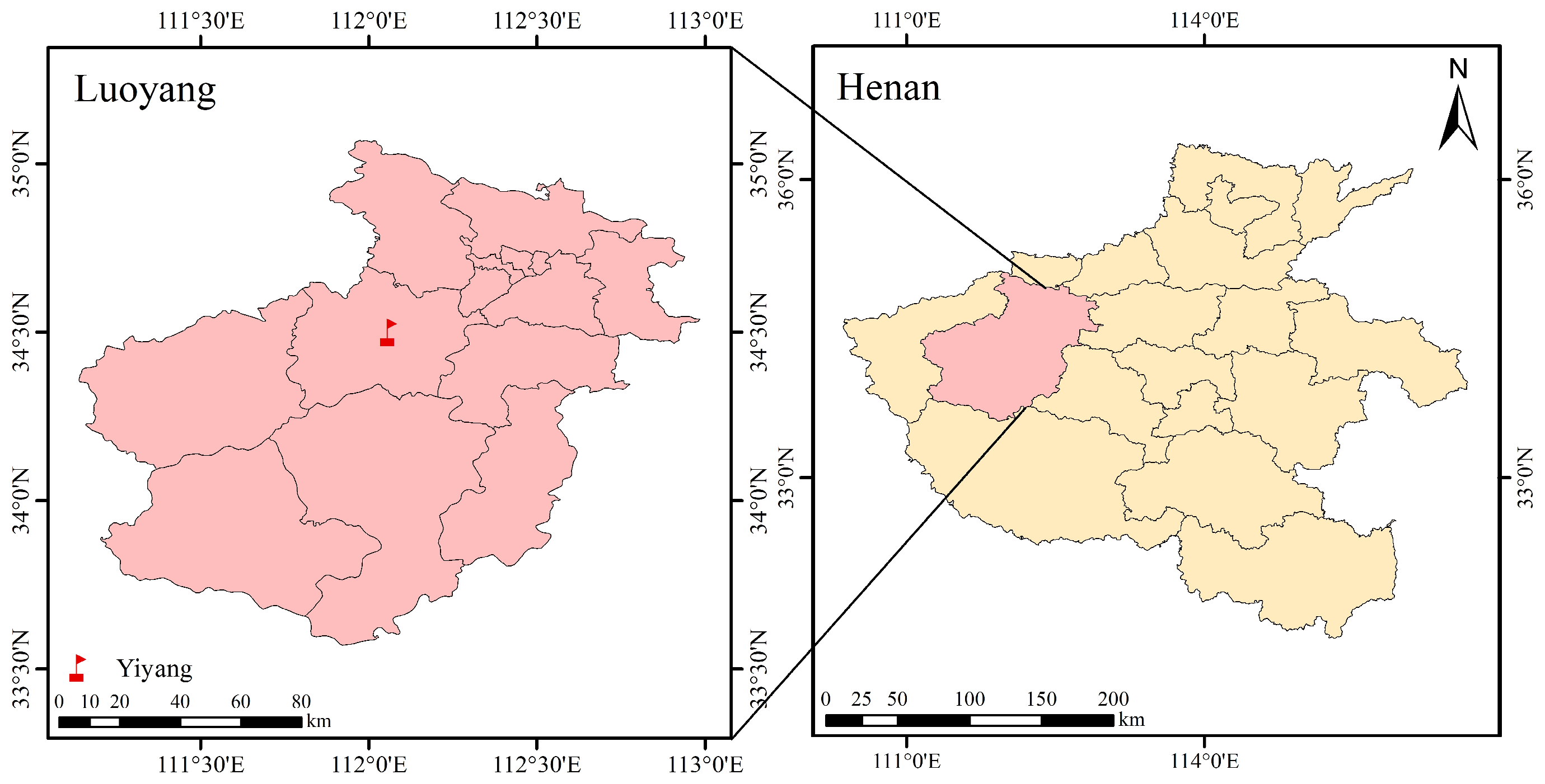
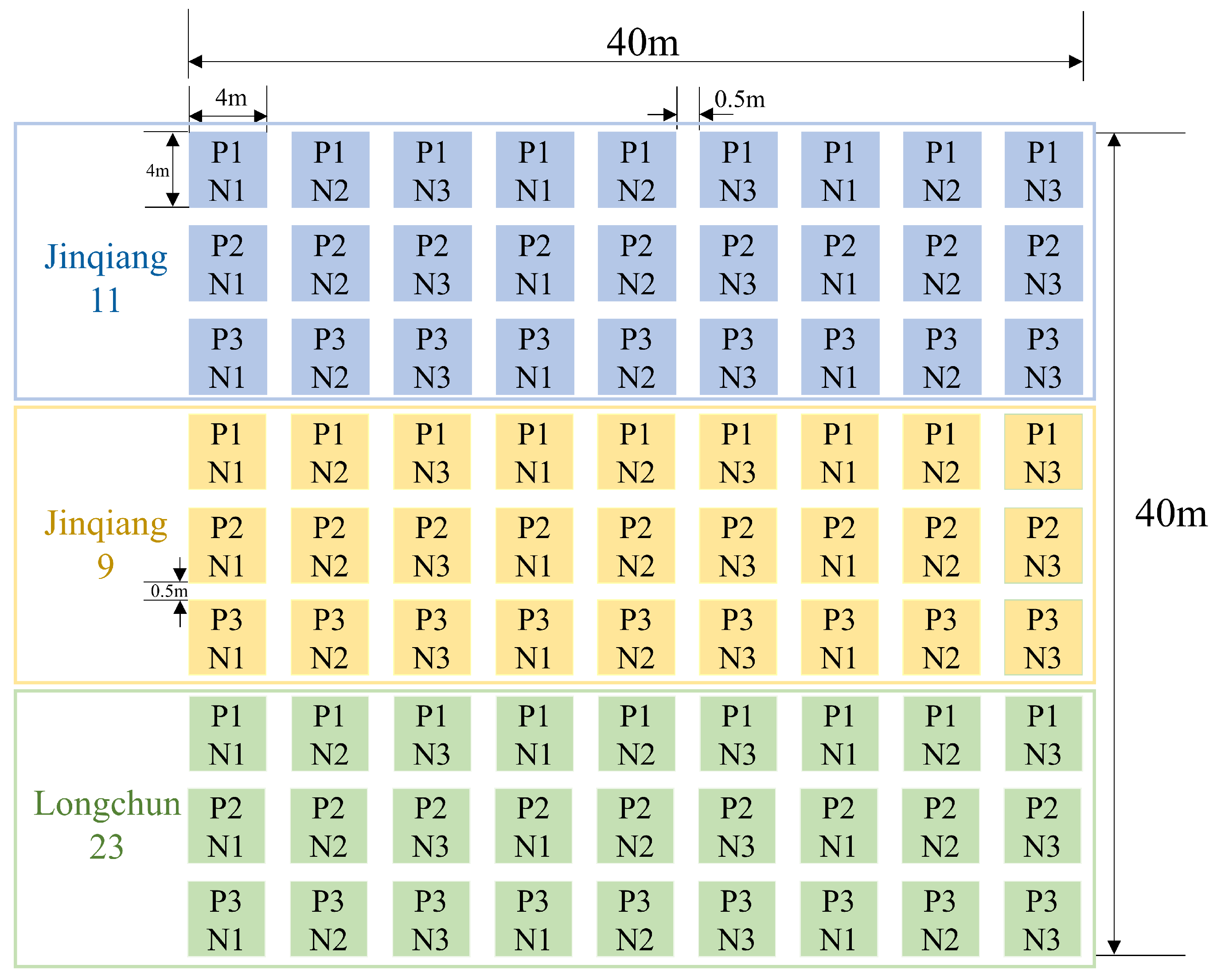
The field experiment was carried out at the China National Tractor Corporation Smart Agriculture Demonstration Park, Lianzhuang Town, Yiyang County, Luoyang City, Henan Province, China (34°47′ N, 112°37′ E, 223 m). The study site experiences a temperate continental monsoon climate, averaging approximately 15 °C and 648 mm of precipitation annually (Figure 1 [29]). Experiments were conducted in large fields of the park between March and July 2023. Three wheat varieties, namely Jinqiang 11 [30], Jinqiang 9 [31] and Longchun 23 [32], were managed in the same way as those in the local conventional farmland, with irrigation, fertilisation and pest and weed control. To increase phenotypic differences in wheat in the experimental area, nitrogen was applied at three rates: 150, 210 and 270 kg/hm² [33], marked as N1, N2 and N3, respectively. In addition, three planting densities were established: 1, 1.6 and 2.2 million plants/hm², referred to as P1, P2 and P3, respectively. Plot planting was implemented according to a full-factorial experimental design, with three replicates per treatment scheme, resulting in 81 plots (each 16 m²) (Figure 2).

2.2. Data Collection

UAV multi-spectral imagery and corresponding field measurements were acquired at four critical growth stages: jointing, booting, heading and filling. The yield data were collected on 3 July 2023. The mapping of growth stages to the BBCH scale, a standardised phenological scale for plant development [34], is shown in

Table 1. Mapping of winter wheat growth stages to the BBCH scale and data collection dates.

Growth Stage	Stage Description	BBCH Scale	Observation Date
Jointing	Stem elongation with detectable nodes	BBCH 30–39	26 April 2023
Booting	Flag leaf sheath swelling preceding heading	BBCH 40–49	8 May 2023
Heading	Spike emergence	BBCH 50–59	17 May 2023
Filling	Grain filling with dry matter accumulation	BBCH 70–79	24 May 2023

.

2.2.1. Multi-Spectral Imagery Data

Multi-spectral imagery of the study area was acquired using a DJI Phantom 4 Multi-spectral (DJIP4M; DJI Technology Co., Ltd., Shenzhen, China) platform. This system integrates six 1/2.9-inch CMOS sensors, each with 2.12 million total pixels (2.08 million effective), including one RGB sensor and five narrowband monochrome sensors. DJIP4M uses a colour sensor for visible imaging and a five-channel multi-spectral sensor to accurately capture multi-spectral images in five spectral bands: blue (450 ± 16 nm), green (560 ± 16 nm), red (650 ± 16 nm), red edge (730 ± 16 nm) and near-infrared (840 ± 16 nm).

Images were collected from 10:00 a.m. to 2:00 p.m. on clear and cloudless days under windless or light-wind conditions. Flights were conducted at a 30 m altitude with 80% forward and a lateral overlap of 70%. Radiometric calibration employed MAPIR reference panels (MAPIR, Inc., San Diego, CA, USA) with reflectances of 25%, 50%, 75%, and 95%. Shadow-free calibration images were obtained at a distance seven times the panel length.

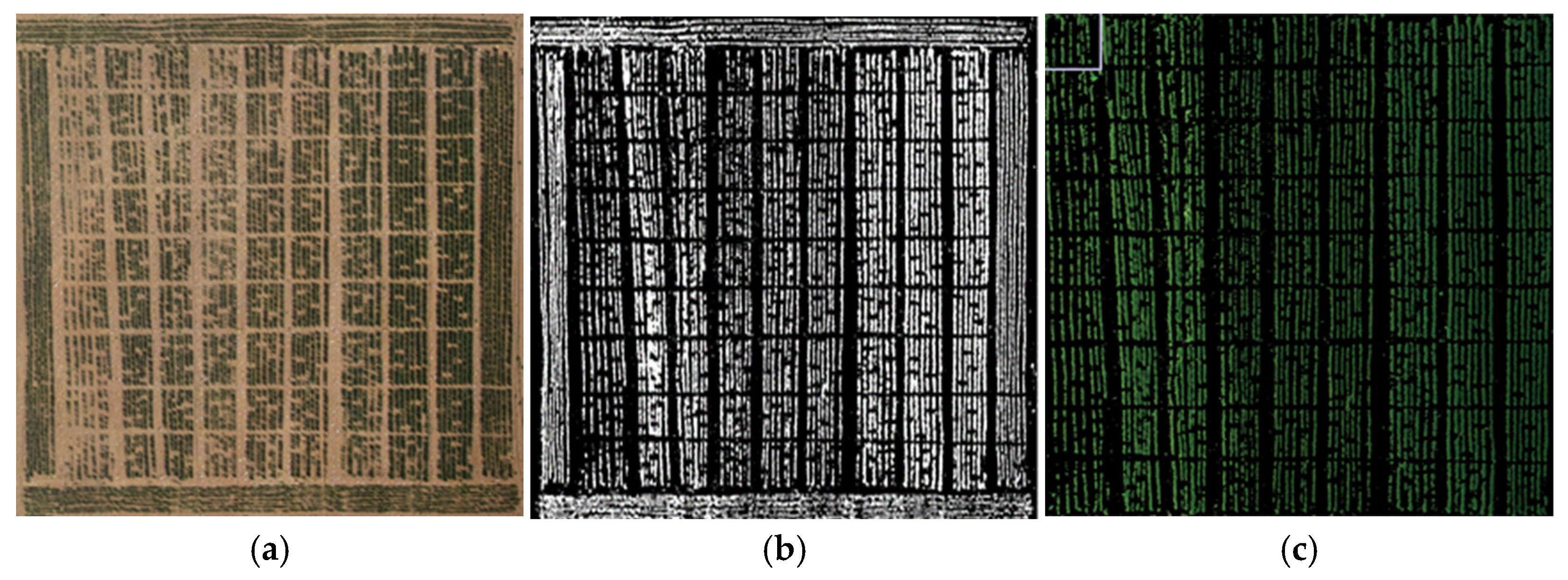
The multi-spectral images were subsequently processed through image stitching, radiation correction, geometric correction, vegetation masking, and extraction of regions of interest (ROIs). Image mosaicking was performed using DJI Terra version 3.7.6 (DJI Technology Co., Ltd., Shenzhen, China). A G970II Pro RTK–GNSS unit (Beijing UniStrong Science and Technology Corporation Limited, Beijing, China) was employed to survey the control-point coordinates with centimetre-level accuracy, after which the images were geometrically rectified in ENVI version 5.3.1 (Exelis Visual Information Solutions, Inc., Broomfield, CO, USA). Image cropping, vegetation masking and ROI extraction were conducted in MATLAB R2024a (The MathWorks, Inc., Natick, MA, USA). To remove non-vegetation background interference, a growth-stage-specific spectral threshold segmentation method was applied. Because canopy architecture and spectral responses evolved as the crop developed, appropriate spectral indices and thresholds were determined for vegetation extraction. Specifically, green-band reflectance was used for vegetation masking at the jointing stage, NDVI was applied at the booting stage, and EVI was used for the heading and filling stages. The corresponding thresholds were empirically determined according to the spectral differences between wheat canopy and background regions. Pixels satisfying the predefined threshold criteria were retained as vegetation pixels, and the generated binary masks were applied to all spectral bands to remove background interference. Subsequently, the experimental area was divided into 81 plots using a 9 × 9 regular grid, and plot-level ROIs were extracted. The wheat canopy reflectance spectra within each sampling plot were then obtained for subsequent analysis (Figure 3).

2.2.2. Wheat Growth and Yield Measurements

Growth indicators are time-sensitive [35]. Field measurements of stem tiller density, LAI, AGB and wheat yield, were collected at four key growth and harvest stages.

Stem tiller density was measured using quadrat sampling methods. A 0.5 m × 0.5 m wooden frame was used to randomly select areas with relatively uniform growth within each plot. The number of tillers with no fewer than three leaves in the selected area was recorded, and tiller count was converted into stem tiller density per unit area.

LAI was determined non-destructively using a SunScan canopy analyser (Delta-T Devices Ltd., Cambridge, UK). Within each plot, four sampling locations were evenly spaced: two at the ridge tops, and two at one-third and two-thirds of the distance down between ridges. At each location, three replicate readings were taken, and the plot-specific mean was calculated as the LAI value. To minimise errors from direct sunlight, data were collected between 06:30 and 09:30 and between 16:30 and 19:30.

AGB was measured by destructive sampling and oven-drying. Within each plot, random placement of a 0.5 m × 0.5 m wooden frame defined a relatively uniform sampling area. The above-ground wheat within the frame was harvested and immediately weighed for fresh weight. Subsequently, samples were bagged, carried to the lab, and dried in an oven. Drying began at 105 °C for 30 min, followed by 80 °C until a stable mass was obtained. Dry mass was measured and standardised to above-ground biomass per unit area (t/ha).

Yield data were acquired from manual plot harvesting at maturity. A total of 1 m² of wheat was randomly selected from each plot for manual harvesting, threshing, drying and weighing. The yield data were then converted to yield per unit area (kg/ha) using the planting density. The yield data used refer to wheat grain yield.

2.3. Construction of CGIs

Given the inconsistency in wheat agronomic parameters for CGI construction, the need for objective weighting and for accounting for correlations between indicators, the CRITIC weighting method was used to construct the CGI for wheat based on the importance of wheat stem tiller density, LAI and AGB. For comparison, the coefficient of variation method was also applied.

2.3.1. Construction of CGI_CR Using the CRITIC Weighting Method

The CRITIC weighting method [36] is an objective weighting approach that relies on data volatility. Its fundamental concept involves two indicators, volatility (contrast intensity) and conflict (correlation), which comprehensively assess the objective weight of each indicator. Volatility is quantified by the standard deviation. A high standard deviation indicates high volatility, resulting in a high weight. This quantifies the importance of different indicators for yielding objective decision outcomes and effectively handles changes in criterion weights. By adjusting weights, different decision outcomes can be obtained under various conditions. Conflict is represented using a correlation matrix. A high value for the phase relation between indicators represents high similarity between the indicators, and a low conflict indicates a low weight. This considers the correlation between the indicators, minimises decision-making bias and improves the accuracy of decision-making. CGI_CR is calculated as follows:

$$S_j=\sqrt{{\displaystyle \frac{{{\sum }_{i-1}^n(X_{ij}-{\overline{X}}_j)}^2}{n-1}}}$$

(1)

where $S_j$ represents the standard deviation for the $j$-th indicator, indicating the variability of the indicator; $X_{ij}$ represents the value of the $j$-th evaluation indicator for the $i$-th sample; and ${\overline{X}}_j$ represents the mean for the $j$-th indicator.

$$R_j={\sum }_{i=1}^P(1-r_{ij})$$

(2)

$$C_j=S_j\times R_j$$

(3)

$$W_j={\displaystyle \frac{c_j}{{\sum }_{i=1}^P{c}_j}}$$

(4)

where $r_{ij}$ denotes the correlation coefficient between indicators $i$-th and $j$-th; $P$ represents the number of indicators; $C_j$ is the information-carrying capacity of the $j$-th indicator; and $W_j$ represents the final objective weight of the $j$-th indicator.

After calculation, the CGI_CR expressions for the different growth stages were as follows:

$$\mathrm{Jointing}\mathrm{stage}:{CGI}_{CR}=0.2886I_1+0.4197I_2+0.2917I_3$$

(5)

$$\mathrm{Booting}\mathrm{stage}:{CGI}_{CR}=0.1882I_1+0.485I_2+0.3267I_3$$

(6)

$$\mathrm{Heading}\mathrm{stage}:{CGI}_{CR}=0.2268I_1+0.4554I_2+0.3178I_3$$

(7)

$$\mathrm{Filling}\mathrm{stage}:{CGI}_{CR}=0.2193I_1+0.5157I_2+0.2649I_3$$

(8)

where $I_1$, $I_2$ and $I_3$ are normalised stem tiller density, LAI and AGB, respectively.

2.3.2. Construction of CGI_CV Using the Coefficient of Variation Method

The coefficient of variation method determines the weight of an indicator from the information contained in the variability of its values. As the indicator value changes, its weight changes accordingly, which makes this approach dynamic and objective. The resulting weights are dimensionless [37]. The expressions for CGI_CV at different growth stages were as follows:

$$\mathrm{Jointing}\mathrm{stage}:{CGI}_{CV}=0.3761I_1+0.3124I_2+0.3115I_3$$

(9)

$$\mathrm{Booting}\mathrm{stage}:{CGI}_{CV}=0.3699I_1+0.3279I_2+0.3022I_3$$

(10)

$$\mathrm{Heading}\mathrm{stage}:{CGI}_{CV}=0.3446I_1+0.3495I_2+0.3059I_3$$

(11)

$$\mathrm{Filling}\mathrm{stage}:{CGI}_{CV}=0.347I_1+0.3738I_2+0.2792I_3$$

(12)

2.4. Selection of VIs

Given the low correlation observed between individual spectral bands and crop growth indicators during the initial phase of this study, along with the demonstrated superiority of VIs in capturing crop biophysical parameters [38,39], VIs were selected to estimate wheat growth.

Current studies using multi-spectral VIs for estimating crop yield are classified into the following categories [27]: (1) multi-spectral indices based on the red and near-infrared wavelengths, which effectively reflect crop growth status and photosynthesis, including Normalised Difference VI (NDVI), Ratio VI (RVI), Difference VI (DVI), Enhanced VI (EVI), and its improved version Enhanced VI 2 (EVI2); (2) multi-spectral indices that account for the influence of soil background on vegetation characteristics, which are effectively applicable for yield estimation under complex surface conditions, including Soil-Adjusted VI (SAVI), Optimised Soil-Adjusted VI (OSAVI) and Green Soil-Adjusted VI (GSAVI); (3) multi-spectral indices that emphasise the sensitivity of the red-edge spectrum, providing a relatively accurate assessment of crop health, including Simple Red-Edge Ratio Index (SRREDEDGE), Red-Edge Chlorophyll Index (CLrededge), Normalised Red-Edge Index (NREI) and MERIS Terrestrial Chlorophyll Index; (4) multi-spectral indices based on spectral variation from green to near-infrared wavelengths, which reveal changes in chlorophyll and photosynthetic dynamics at different growth stages of crops, making them useful for growth monitoring and yield prediction, including Green Normalised Difference VI (GNDVI), Green Ratio VI (GRVI) and Green Leaf Index (GLI); (5) VIs reflecting leaf pigment content, which are useful for monitoring crop development and predicting yield, including Chlorophyll Green Index (CLgreen) and Modified Chlorophyll Absorption Ratio Index (MCARI); and (6) VIs related to water content (WI) and other indices.

In view of the unique application value of the numerous VIs mentioned above, the spectral reflectance of 81 test areas was extracted in this study, and 32 VIs were calculated using relevant equations (

Table 2. Equations of the vegetation indices.

Vegetation Index	Equation	References
CIVE	$CIVE=0.441\times R_{650}-0.881\times R_{560}+0.385\times R_{450}+18.78745$	[40]
CLgreen	$CLgreen=(R_{840}/R_{560})-1$	[41]
CLrededge	$CLrededge=(R_{840}/R_{730})-1$	[41]
DATT	$DATT=(R_{840}-R_{730})/(R_{840}-R_{650})$	[42]
DVI	$DVI=R_{840}-R_{650}$	[43]
ENDVI	$ENDVI=(R_{840}+R_{560}-2\times R_{450})/(R_{840}+R_{560}+2\times R_{450})$	[44]
EVI	$EVI=2.5\times$ ($R_{840}-R_{650}$)/(1 + $R_{840}+6\times R_{650}-7.5\times R_{450}$)	[45]
EVI2	$EVI2=2.4\times (R_{840}-R_{650})/(R_{840}+R_{650}+1)$	[46]
ExG	$ExG=2\times R_{560}-R_{650}-R_{450}$	[47]
GLI	$GLI=$($2\times R_{560}-R_{650}-R_{450}$)/($2\times R_{560}+R_{650}+R_{450}$)	[48]
GNDVI	$GNDVI=(R_{840}-R_{560})/(R_{840}+R_{560})$	[49]
GRVI	$GRVI=R_{840}/R_{560}$	[50]
GSAVI	$GSAVI=1.5\times (R_{840}-R_{560})/(R_{840}+R_{560}+0.5)$	[51]
MCARI	$MCARI={\displaystyle \frac{(\left(R_{730}-R_{650}\right)-(0.2\times (R_{730}-R_{560})\left)\right)\times R_{730}}{R_{650}}}$	[52]
MCARI2	$MCARI2={\displaystyle \frac{1.5\times (2.5\times \left(R_{840}-R_{650}\right)-1.3\times (R_{840}-R_{730}\left)\right)}{\sqrt{{(2\times R_{840}+1)}^2-\left(6\times R_{840}-5\times \sqrt{R_{650}}\right)-0.5}}}$	[52]
MDD	$MDD=(R_{840}-R_{730})/(R_{730}-R_{560})$	[53]
MEVI	$MEVI={\displaystyle \frac{2.5\times (R_{840}-R_{730})}{(R_{840}+6\times R_{730}-7.5\times R_{560}+1)}}$	[54]
MNVI	$MNVI=(1.5\times {R_{840}}^2-1.5\times R_{650})/({R_{840}}^2+R_{650}+0.5)$	[54]
MNDI	$MNDI=(R_{840}-R_{730})/(R_{840}-R_{560})$	[54]
MNLI	$MNLI=(1.5\times {R_{840}}^2-1.5\times R_{560})/({R_{840}}^2+R_{650}+0.5)$	[55]
MTCI	$MTCI=(R_{840}-R_{730})/(R_{730}+R_{650})$	[56]
NDVI	$NDVI=\left(R_{840}-R_{650}\right)/\left(R_{840}+R_{650}\right)$	[49]
NNIR	$NNIR=R_{840}/(R_{840}+R_{650}+R_{730})$	[51]
NGI	$NGI=R_{560}/(R_{840}+R_{560}+R_{730})$	[51]
NLI	$NLI=({R_{840}}^2-R_{650})/({R_{840}}^2+R_{650})$	[57]
NREI	$NREI=R_{730}/(R_{840}+R_{560}+R_{730})$	[54]
OSAVI	$OSAVI=\left(R_{840}-R_{650}\right)/\left(R_{840}+R_{650}+0.16\right)$	[58]
RTVICore	${RTVI}_{Core}=100\times \left(R_{840}-R_{730}\right)-10\times (R_{840}-R_{560})$	[59]
RVI	$RVI=R_{840}/R_{650}$	[60]
SAVI	$SAVI={\displaystyle \frac{R_{840}-R_{650}}{R_{840}+R_{650}+0.5}}\times (1+0.5)$	[61]
SRREDEDGE	$SRREDEDGE=R_{840}/R_{730}$	[62]
WI	$WI=$($R_{560}-R_{450}$)/($R_{650}+R_{560}$)	[62]

Note: $R_{450}$, $R_{560}$, $R_{650}$, $R_{730}$ and $R_{840}$ represent the reflectance values of blue, green, red, red-edge and near-infrared wavelengths, respectively.

). Considering that the relationships between VIs and yield are not strictly linear, preliminary screening of VIs at critical growth stages was conducted based on previous Pearson correlation analysis results [29]. Subsequently, Shapley Additive exPlanations (SHAP) analysis was further performed to identify key features from a model interpretation perspective and to assess their importance within the machine learning model. Both methods were applied to the selected VIs using MATLAB.

2.5. Yield Estimation Models

KELM and CPO-KELM were employed for wheat yield estimation. All computations were performed in MATLAB R2024a, with the Statistics and Machine Learning Toolbox version 24.1 used for kernel function implementation and the Parallel Computing Toolbox version 24.1 for computational acceleration. To prevent data leakage, modelling was conducted at the plot level. For each of the 81 plots, the VIs and CGI from the four growth stages were concatenated into a single feature vector and paired with the corresponding yield. Data splitting was performed after the plot-level feature vectors were constructed. The resulting 81 samples were randomly divided into training and validation sets at a ratio of 7:3. This procedure guarantees that all information belonging to a given plot is exclusively assigned to one subset. Model parameters were calibrated using the training subset, whereas predictive performance was assessed using the validation subset, which was excluded from the training process.

2.5.1. Kernel Extreme Learning Machine (KELM)

KELM incorporates kernel functions into the extreme-learning machine model to improve its capability for nonlinear prediction. Through implicit feature mapping, input samples are projected into a higher-dimensional feature space, where nonlinear relationships can be represented more effectively. Instead of explicitly constructing hidden-layer parameters, KELM directly calculates the kernel matrix in the feature space, thereby reducing computational complexity and alleviating the influence of dimensionality on model performance [63,64]. The radial basis function was selected as the kernel function. The regularisation coefficient C and kernel parameter S were determined using a grid-search procedure, and both parameters were set to 100. This parameter combination exhibited optimal predictive stability on the validation set, effectively balancing model complexity and generalisation capability [65]. However, despite improvements in the generalisation ability and stability of the model through KELM, how to effectively optimise the kernel function for enhancing performance has not been resolved.

2.5.2. KELM Based on the Crested Porcupine Optimizer (CPO-KELM)

To enhance predictive performance, the Crested Porcupine Optimizer (CPO), a metaheuristic algorithm proposed by Abdel-Basset et al. [66] in 2024, was used to optimise the hyperparameters of KELM (regularisation coefficient C and kernel parameter S). The algorithm implementation followed the configuration described by Chen et al. [67].

The search space was optimised using CPO for KELM, with the optimal selection of C ∈ [0.1, 1800] and S ∈ [0.1, 1800]. The population size and maximum number of iterations were set to 50. The dynamic adjustment coefficient ($\alpha$) and phase transition threshold ($T_f$) were set to 0.2 and 0.8, respectively.

In the initialisation stage, 50 candidate solutions (C and S combinations) were randomly generated within the search space to form the initial population. The population size was dynamically adjusted according to Equation (13), with the adjustment period determined by parameter T = 2. As the iterations proceeded, the population size was systematically reduced to enhance local search efficiency. Global exploration was performed with a probability of 0.8, using random sampling and differential mutation to maintain search diversity. In the local exploration phase (probability $1-T_f$), the search direction was guided by elite individuals, with the convergence rate controlled by $\alpha$ = 0.2 to prevent premature convergence. After each iteration, the parameter values were verified and any parameter outside the [0.1, 1800] range was randomly reassigned to a value within the valid bounds.

The mean squared error (MSE) of the training set was used as the fitness function, with lower values indicating better predictive performance. During optimisation, the MSE was recorded at each iteration. After 50 iterations, the optimal parameter combination (C and S) yielding the minimum MSE was identified. These optimised parameters were then used to validate model performance on the independent validation dataset.

$$N=N_{min}+\left(N^{\prime }-N_{min}\right)\times \left(1-\left({\displaystyle \frac{t\%\frac{T_{max}}{T}}{\frac{T_{max}}{T}}}\right)\right)$$

(13)

where $T$ represents the variable determining the number of iterations; $T_{max}$ denotes the maximum number of function evaluations; $t$ represents the current function evaluation; $\%$ represents the modulus operator; and $N_{min}$ refers to the minimum number of individuals in the newly generated population, ensuring that the population size is not smaller than $N_{min}$.

Considering the characteristics of KELM and CPO, this study used KELM and CPO-KELM to develop the wheat yield estimation model.

To evaluate the potential impact of information leakage during CPO optimisation, an additional internal validation experiment was conducted. Within the training data, 80% of the samples were assigned to a sub-training subset and the remaining 20% to an internal-validation subset, and the CPO fitness function was redefined using only the internal validation error. Fifty independent optimisation runs were performed, each initialised with a distinct random seed. Detailed outcomes are reported in Supplementary Figures S1 and S2 and Supplementary Table S1.

2.5.3. Evaluation of Multi-Period Feature Redundancy and Design of Stage-Level Ablation Experiments

Since the multi-period remote sensing features and composite agronomic indicators may have information overlap in the time series, resulting in some input variables containing similar growth information and potentially reducing the model’s ability to identify effective features, this study further designed feature redundancy assessment and stage-level ablation experiments.

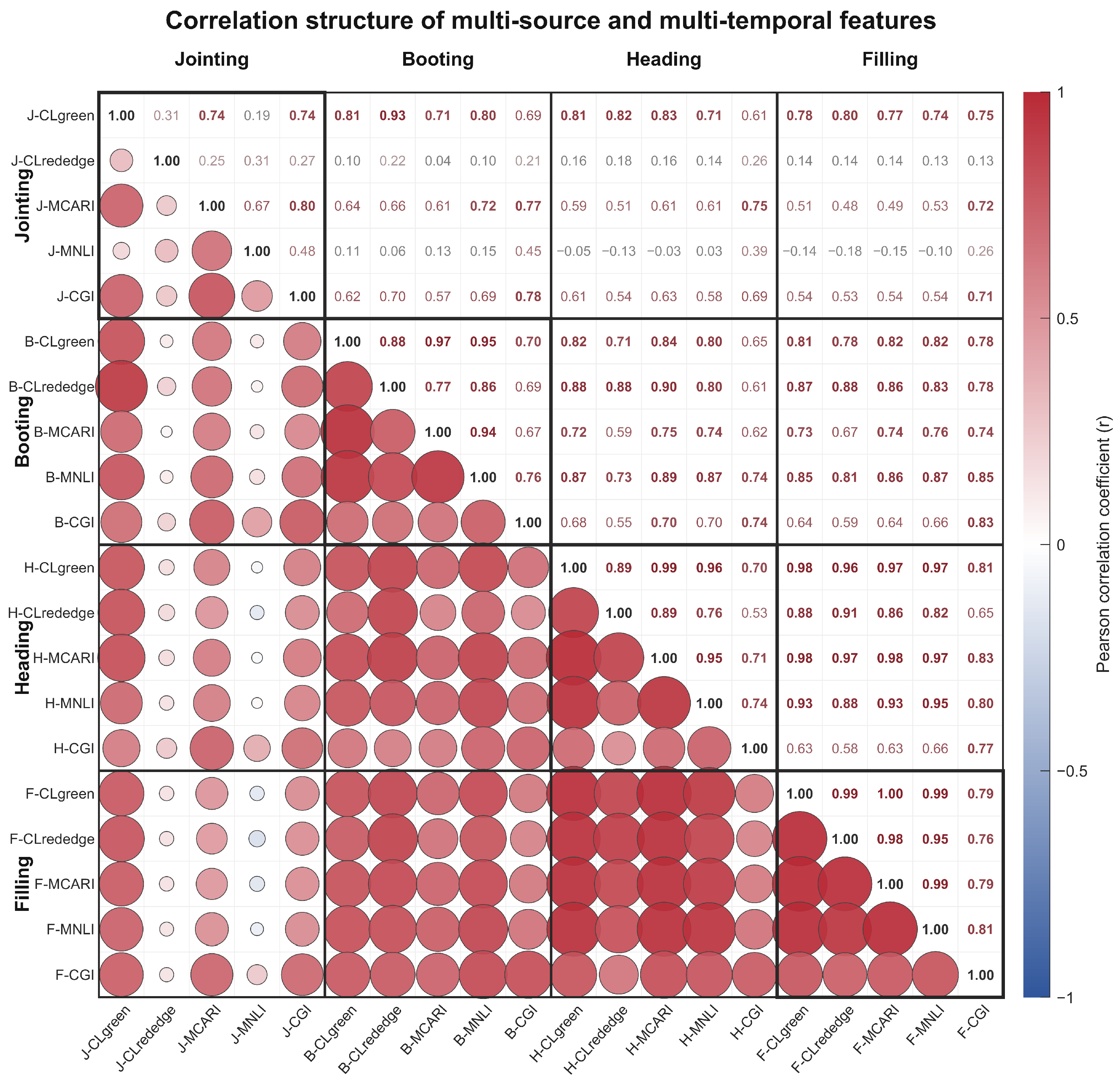
Firstly, pairwise Pearson coefficients were estimated for the 20 variables, comprising four sensitive VIs and one CGI_CR from each of the four growth stages. The resulting coefficients were organised into a matrix and displayed as a combined bubble-and-number heatmap to assess collinearity across growth stages and feature types.

Secondly, to clarify the incremental contribution of each growth period and feature type to the final yield, stage-level ablation experiments based on CPO-KELM were designed. Using the model (ALL_FULL) that integrates all four growth periods’ VIs and CGI_CR features as the baseline model, the features of the jointing stage, booting stage, heading stage, and filling stage were removed, and the model was retrained to evaluate the incremental contribution of each growth stage to the final yield estimation. At the same time, to further analyse the information contribution of key growth stage combinations, single-stage models and stage combination models (such as heading and filling stage) were constructed, and the performance differences in the models under different time windows were compared. Additionally, by removing different types of feature sources (VIs or CGI_CR), the effect of integrating remote-sensing information from multiple sources on model prediction ability was evaluated.

All ablation experiments used 100 random data partitions (70% training set, 30% validation set), and the performance differences between different feature combination models under the same modelling conditions were compared, and the performance changes and their 95% confidence intervals were calculated to quantitatively evaluate the contribution of different growth stages and feature types to the model’s predictive ability.

2.6. Model Evaluation

Three metrics were used to assess model performance following Equations (14)–(16): the coefficient of determination (R²), root mean square error (RMSE) and relative prediction deviation (RPD). R² measures the agreement between actual and predicted values, with values ranging from 0 to 1; a value closer to 1 indicates a stronger fit. RMSE quantifies the extent to which predicted values deviate from actual ones. A high R² indicates low RMSE and high prediction accuracy [68]. RPD is the ratio of the sample standard deviation to RMSE. The model’s predictive ability was classified into three levels: type A (RPD > 2; good predictive ability), type B (1.4 ≤ RPD ≤ 2; moderate predictive ability, providing a rough prediction of the samples) and type C (RPD < 1.4; poor predictive ability).

Mean relative error (MRE) was used to assess model stability. A low MRE indicated that the predicted results are close to the actual values, with reduced volatility and high resistance to interference, thereby reflecting high stability.

$$R^2={\displaystyle \frac{{\left[{\sum }_{i=1}^n(x-\overline{x})(y-\overline{y})\right]}^2}{{\sum }_{i=1}^n{(x-\overline{x})}^2{\sum }_{i=1}^n{(y-\overline{y})}^2}}$$

(14)

$$RMSE=\sqrt{{\displaystyle \frac{{\sum }_{i=1}^n{(x-y)}^2}{n}}}$$

(15)

$$RPD={\displaystyle \frac{SD}{RMSE}}$$

(16)

$$MRE={\displaystyle \frac{1}{n}}{\displaystyle \sum _{i=1}^n}\left|{\displaystyle \frac{x-y}{y}}\right|$$

(17)

where $x$ represents the predicted value; $\overline{x}$ represents the mean of predicted values; $y$ represents the observed value; $\overline{y}$ represents the mean of observed values; and $n$ represents the sample size.

3. Results

3.1. Feature Selection

3.1.1. Identification of VIs at Critical Growth Stages and SHAP Analysis

Pearson correlation analysis revealed that across the four key growth stages (jointing, booting, heading and filling), the VIs most strongly associated with yield were CLgreen, CLrededge, MCARI and MNLI [29].

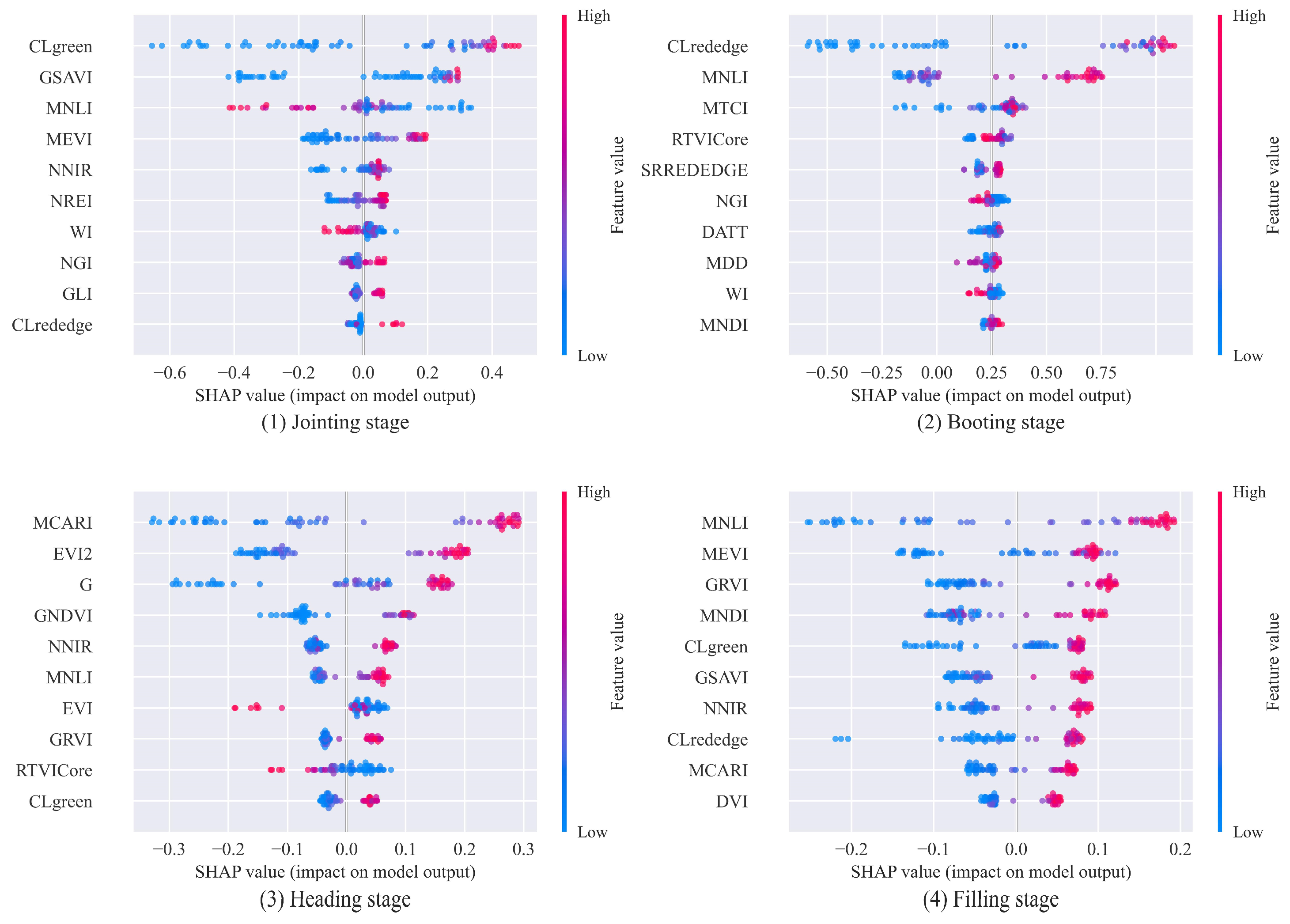
To evaluate the contributions of these VIs to the machine learning model, a SHAP analysis was further conducted. As shown in Figure 4, SHAP not only quantified the global importance of each VI but also illustrated how feature values influenced yield prediction. The results indicated that at each growth stage, the VIs with the highest SHAP values were CLgreen (jointing), CLrededge (booting), MCARI (heading) and MNLI (filling), consistent with the Pearson correlation results. This consistency between the two analytical approaches supports the reliability of these VIs as key predictors of wheat yield.

3.1.2. Correlation Analysis of Yield with CGIs and Individual Agronomic Parameters

Spearman’s rank correlation was employed to evaluate the relationships among CGI_CV, CGI_CR and yield data. The results are shown in

Table 3. Correlation coefficients between CGI_CV, CGI_CR and yield across different periods.

Growth Stage	CGICV	CGICR
Jointing	0.479 **	0.499 **
Booting	0.630 **	0.701 **
Heading	0.657 **	0.718 **
Filling	0.806 **	0.846 **

Note: ** indicate extremely significant correlations at the 0.01 level (p < 0.01).

.

As shown in Table 3, the two CGI types were strongly correlated with yield across the four periods. Across the jointing to filling stages, the correlation coefficient between yield and CGI gradually increased, reaching a maximum at the filling stage. CGI_CV correlated with yield at 0.806, and CGI_CR at 0.846. At each growth stage, a higher correlation coefficient with yield was found for CGI_CR than for CGI_CV.

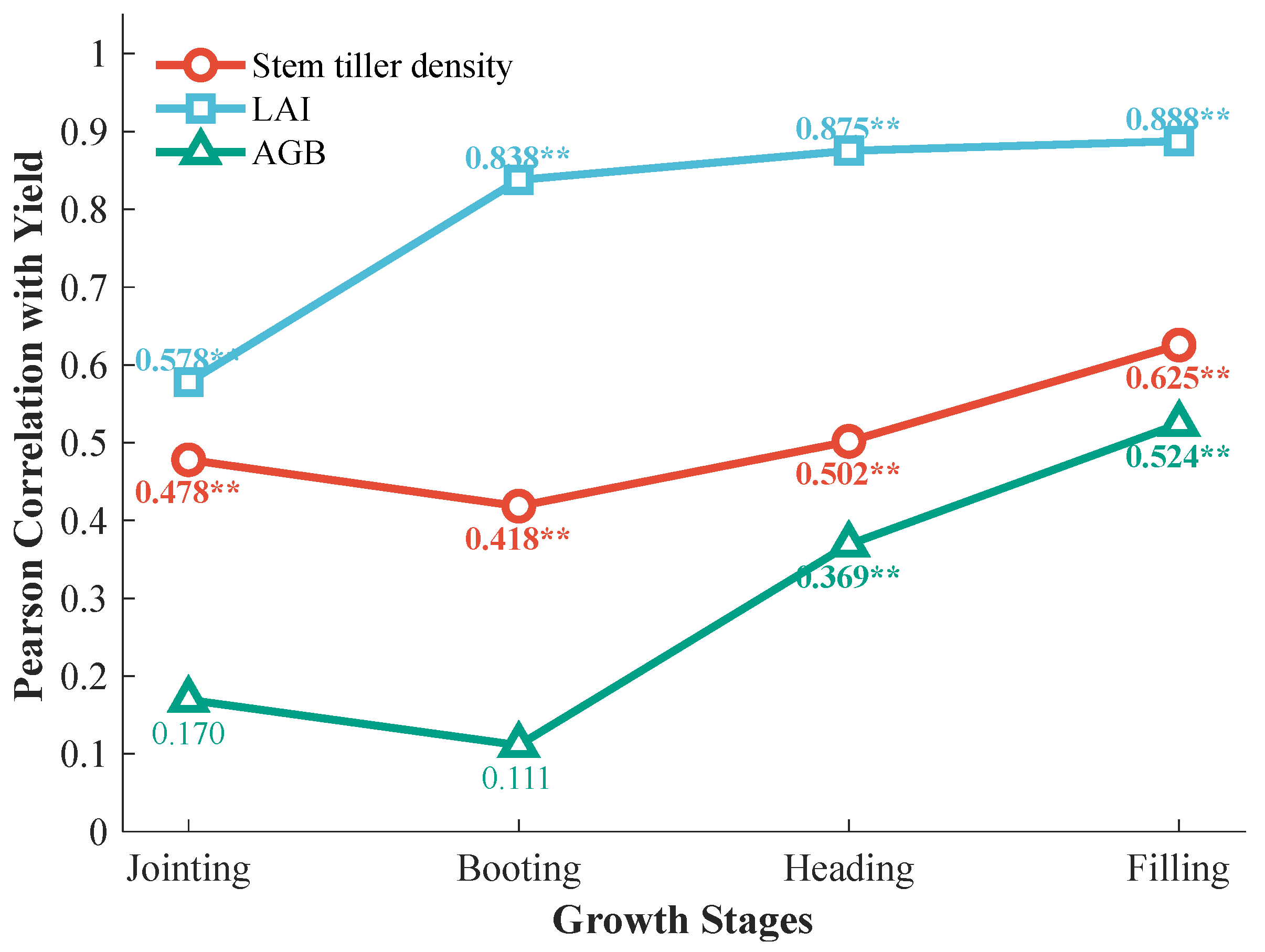
The contributions of individual agronomic parameters were evaluated by analysing their dynamic Pearson correlations with yield across the four growth stages (Figure 5). Distinct temporal behaviours were observed for each variable. Stem tiller density maintained a stable, statistically significant positive correlation across all stages. By contrast, AGB demonstrated non-significant correlations during the jointing and booting stages, but its correlation increased significantly during the heading and filling stages. Despite this weak early-stage correlation, the integration of AGB into the CGI is justified by the CRITIC method, which allocated a substantial and stable weight (0.2649–0.3267) to this parameter based on its independent informational variance. These varying temporal responses confirm that the composite index integrates the complementary characteristics of the three parameters, capturing crop growth features more comprehensively than any single indicator.

3.2. Yield Estimation Model Established Using Parameters at a Single-Growth Stage

3.2.1. Yield Estimation Model Based on VIs

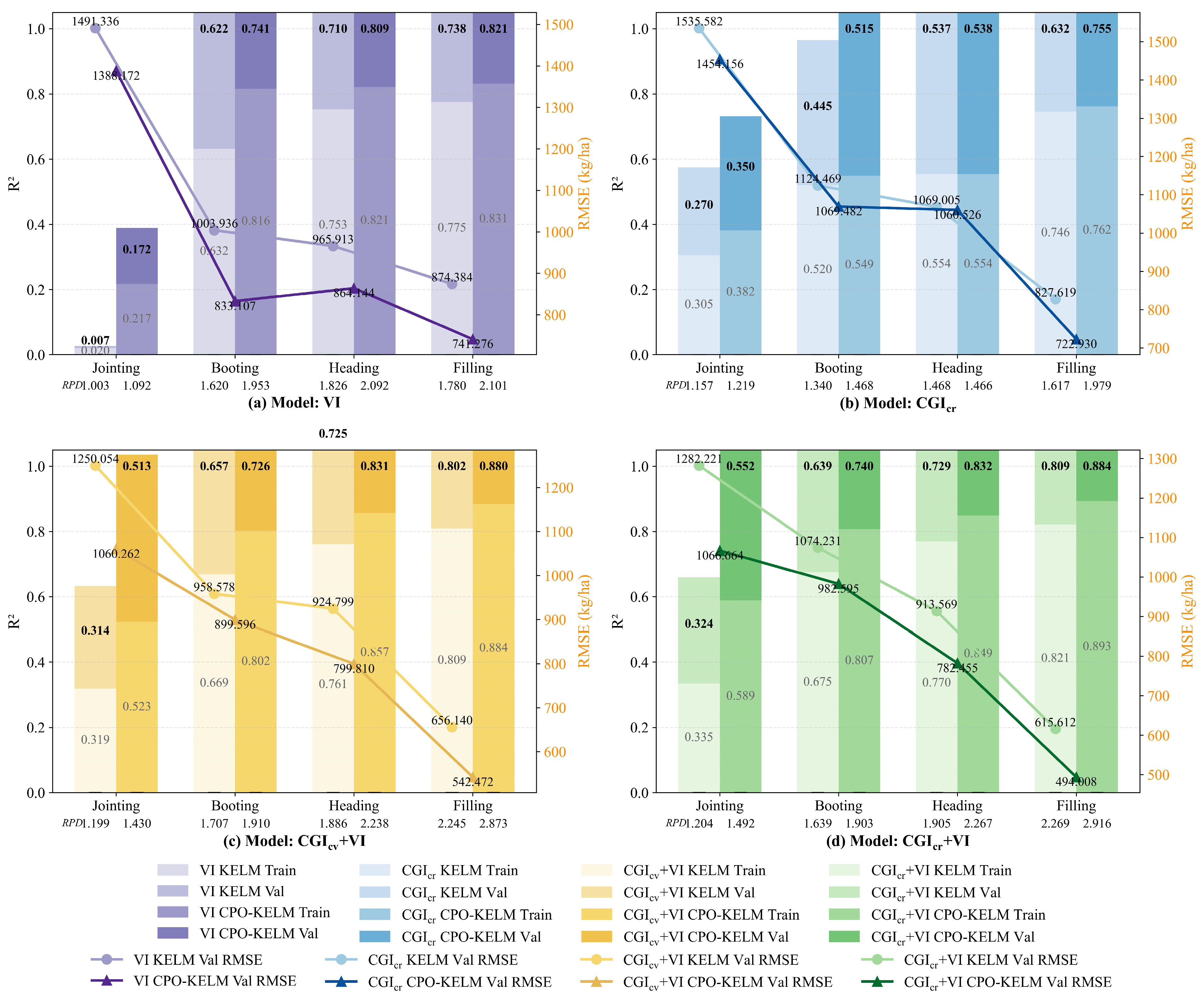
Four VIs exhibiting the highest yield correlation and feature importance were selected as independent variables. Using the KELM and CPO-KELM algorithms, wheat yield estimation models were established for the jointing, booting, heading and filling stages. The dataset was randomly shuffled, and 100 independent random splits were performed, each generating a training and validation pair. The results are shown in Figure 6a.

CPO-KELM consistently outperformed KELM, and predictive performance progressively improved with crop development. The CPO-KELM model was classified as C-type at jointing, B-type at booting, and A-type at heading and filling. At heading and filling, CPO optimisation increased the validation R² by 9.9% and 8.3%, respectively, while reducing RMSE by 101.77 and 133.11. These results indicate that VI-based yield estimation became reliable from the heading stage onward.

3.2.2. Yield Estimation Model Based on CGI_CR

CGI_CR, which was highly correlated with yield, was used as the independent variable. Following the same modelling approach as in Section 3.2.1, KELM and CPO-KELM were applied to estimate wheat yield.

CPO-KELM consistently outperformed KELM in terms of accuracy (Figure 6b). However, none of the CGI_CR-based models reached A-type performance. The filling stage model performed best, with a validation R² of 0.755. Compared with the VI-based model, the CGI_CR-based model performed better only at the jointing stage, where validation R² increased by 0.178. During booting, heading, and filling, the VI-based models remained more accurate, indicating that CGI_CR may provide complementary information for yield estimation at the jointing stage, whereas the selected VIs showed better predictive performance during the later growth stages.

3.3. Yield Estimation Model Using Multi-Source Feature Fusion

To leverage the advantages of both spectral remote sensing and agronomic yield estimation models, a fused yield estimation model was constructed by combining remote sensing VIs and CGI for each growth stage.

3.3.1. Yield Estimation Model Based on CGI_CV and VIs

CGI_CV, together with VIs, were used as inputs to construct yield estimation models for each growth stage (Figure 6c). The fused model outperformed the models using only VIs or only CGI, achieving higher accuracy and RPD across most stages.

At the jointing stage, the validation set R² of the CPO-KELM model increased from 0.172 and 0.350 for the two single-source models to 0.513, whereas RPD increased to 1.430, improving the model from C-type to B-type. At the heading and filling stages, the fused models reached A-type performance, with the best result obtained at filling (R² = 0.880 and RPD = 2.873). However, at the booting stage, including CGI_CV as an independent variable led to a 1.5% decrease in R², an increase of 66.489 in RMSE, and reduced model predictive ability, indicating limited additional predictive value at this stage. Overall, integrating CGI_CV with VIs improved yield estimation at most growth stages, although the effect of multi-source feature fusion was dependent on the growth stage.

3.3.2. Yield Estimation Model Based on CGI_CR and VIs

CGI_CR together with VIs were used as inputs to construct yield estimation models for each growth stage (Figure 6d). The combined model achieved higher accuracy and RPD than the models using only VIs or only CGI at the jointing, heading and filling stages, whereas only a slight change was observed at the booting stage.

At the jointing stage, the validation R² increased from 0.172 and 0.350 for the two single-source models to 0.552, while the model predictive ability improved from C-type to B-type. At the heading and filling stages, the fused models reached A-type performance, with validation R² values of 0.832 and 0.884, respectively. The model constructed by integrating CGI_CR with VIs at the filling stage achieved the best performance, with a validation R² of 0.884, an RMSE of 494.008 and an RPD of 2.916. Compared with the models constructed by integrating CGI_CV with VIs, the models based on CGI_CR and VIs generally achieved slightly higher validation R² values, particularly at the jointing and filling stages (Figure 6c,d), suggesting that CGI_CR may provide more useful complementary information for yield estimation under the conditions evaluated in this study.

3.4. Independent Dataset Testing

3.4.1. Independent Dataset

To further evaluate the predictive performance of the aforementioned single-growth stage and multi-source composite remote sensing yield estimation models, a brand-new independent dataset was used for testing. This dataset was collected from the Wisdom Farm in Yibin District, Luoyang City, Henan Province, China (34°56′ N, 113°01′ E, 215 m) in 2025. Three wheat varieties (Luomai 45, Luomai 28 and Luomai 33) and three planting density levels (1.7, 2.7 and 3.7 million plants/hm²) were used, and a complete randomised block design was adopted, with nine experimental plots, each covering an area of 13.5 m². Field management followed local conventional practices. Data collection was completed on 2 April 2025 (jointing stage), including multi-spectral image data from a UAV with 20 m flight height and field-measured data. Yield measurement was completed on 4 June 2025.

3.4.2. External Testing Results

The yield estimation models based on VIs, CGI_CR or CGI_CR and VIs were tested at the jointing stage using independent datasets. The results are shown in

Table 4. External testing results using independent datasets.

Modelling	KELM			CPO-KELM
	R2	RMSE (kg/ha)	RPD	R2	RMSE (kg/ha)	RPD
VI	0.393	2133.47	0.935	0.527	1733.89	1.150
CGICR	0.186	2086.96	0.956	0.185	1930.94	1.033
CGICR + VIs	0.161	1799.618	1.108	0.482	1679.02	1.188

.

A comparative analysis with jointing-stage yield estimation models (Section 3.2 and Section 3.3) demonstrated that the CPO-KELM model achieved higher accuracy than the conventional KELM, indicating the modified algorithm’s enhanced ability to extract nonlinear relationships from high-dimensional features.

On the independent jointing-stage dataset, the CPO-KELM yield estimation model based on VIs achieved optimal performance (R² = 0.527), significantly outperforming the other models. This discrepancy between the results of this test and those of the validation set may stem from variations in the data distribution and environmental conditions. Although the ranking based on R² differed from that obtained using the internal validation set, the model based on CGI_CR and VIs showed a lower RMSE and higher RPD than the VI-based model, suggesting that multi-source feature integration may contribute to reducing prediction errors under independent jointing-stage conditions. As this independent evaluation was confined to the jointing stage, the external results do not cover the heading and filling stages, where the models performed best internally.

3.5. Yield Estimation Model Using Parameters at Multiple Growth Stages

3.5.1. Yield Estimation Model Based on VIs at Multiple Growth Stages

When estimating crop yield, combining image features across multiple periods achieved relatively high performance. Therefore, sensitive VIs from the four stages were used as model inputs for multi-temporal wheat yield prediction. The results are shown in

Table 5. Yield estimation model using VIs at multiple growth periods.

Model	Training Set		Validation Set
	R2	RMSE (kg/ha)	R2	RMSE (kg/ha)	RPD
KELM	0.795	634.400	0.759	847.757	1.836
CPO-KELM	0.879	486.222	0.829	720.945	2.160

.

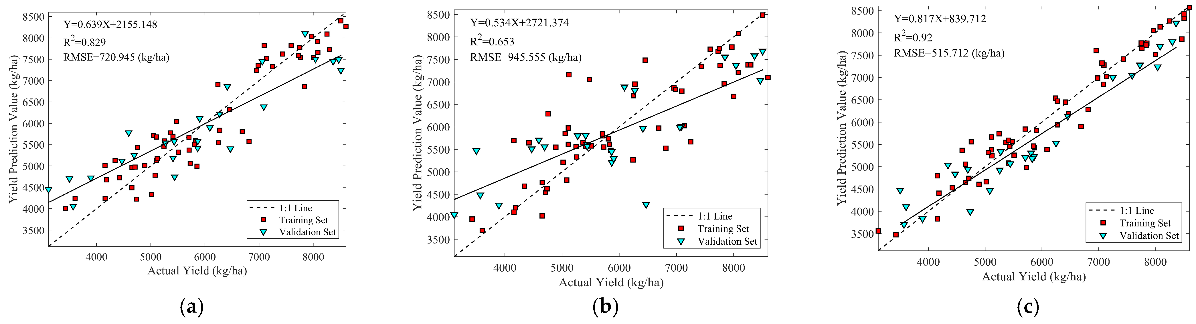
Compared with KELM, CPO-KELM achieved superior performance, with validation R² increasing from 0.759 to 0.829 and RMSE decreasing from 847.757 to 720.945. In addition, RPD increased from 1.836 to 2.160, indicating a transition from B-type to A-type performance. These results demonstrate the effectiveness of CPO optimisation in enhancing model accuracy and stability for multi-temporal yield prediction. Figure 7a demonstrates the relationship between predicted and actual yields of the CPO-KELM model based on VIs at multiple growth stages.

3.5.2. Yield Estimation Model Based on CGI at Multiple Growth Stages

CGI_CR, constructed using the CRITIC weighting method across the four wheat growth stages, was selected as the model input for multi-temporal wheat yield prediction. The results are shown in

Table 6. Yield estimation using CGI_CR at multiple growth stages.

Model	Training Set		Validation Set
	R2	RMSE (kg/ha)	R2	RMSE (kg/ha)	RPD
KELM	0.550	943.555	0.461	1178.403	1.322
CPO-KELM	0.704	760.624	0.653	945.555	1.647

.

Compared with KELM, CPO-KELM remained substantially better performance, with an increase of 19.2% in R² and a decrease of 232.848 in RMSE. Although the model accuracy was still not ideal, it surpassed that of models relying solely on single-temporal images from the jointing, booting and heading stages (Figure 6b). However, its predictive performance remained lower than that of the filling stage model. This result indicates that integrating CGI_CR across multiple growth stages can improve yield estimation relative to models constructed using less informative individual stages, but simply including information from all growth stages does not necessarily produce the best performance. Figure 7b demonstrates the relationship between predicted and actual yields for the CPO-KELM model based on CGI_CR at multiple growth stages.

3.5.3. Yield Estimation Model Based on CGI_CR and VIs at Multiple Growth Stages

Wheat yield prediction was unsuitable during the early growth stages. As shown in Figure 6a,b, the validation set R² values of the CPO-KELM models based on VIs or CGI_CR were <0.5 during the jointing stage. In addition, the R² of the CPO-KELM model based on CGI_CR was <0.6 during the booting stage. Therefore, the CGI_CR for the heading and filling stages, along with the corresponding sensitive VIs, were selected as model inputs for wheat yield estimation. The results are shown in

Table 7. Yield estimation model using CGI_CR and VIs at multiple growth stages.

Model	Training Set		Validation Set
	R2	RMSE (kg/ha)	R2	RMSE (kg/ha)	RPD
KELM	0.835	570.958	0.828	655.453	2.379
CPO-KELM	0.934	360.631	0.920	515.712	3.299

.

The validation set R², RMSE and RPD of the KELM model were 0.828, 655.453 and 2.379, respectively, and those of the CPO-KELM model were 0.920, 515.712, and 3.299, respectively. Both models showed good predictive ability and were classified as A-type models. Compared with KELM, CPO-KELM increased the validation R² by 9.2% and reduced RMSE by 139.741, achieving the best predictive performance in this section. Figure 7c demonstrates a strong agreement between predicted and actual yields for the optimal CPO-KELM model.

3.6. Comprehensive Comparison and Stability Analysis

3.6.1. Comprehensive Comparison and Redundancy Analysis of Feature Fusion Strategies

Comparison of Yield Estimation Models with Different Feature Fusion

To assess the effects of different feature fusion strategies on yield prediction performance, the results of the CPO-KELM model are shown in

Table 8. Performance comparison of CPO-KELM yield estimation models across different growth stages and feature combinations.

Growth Stage	Single-Stage VIs	Single-Stage CGICR	Single-Stage CGICR and VIs	Multi-Stages VIs	Multi-Stages CGICR	Multi-Stage CGICR and VIs
Jointing	0.172	0.350	0.552	0.829	0.653	0.920
Booting	0.741	0.515	0.74
Heading	0.809	0.538	0.832
Filling	0.821	0.755	0.884

Note: Feature sets in this table were pre-filtered using the Variance Inflation Factor (VIF).

.

In the single-growth stage evaluation, relatively low accuracy was observed at the early jointing stage, with progressive improvement as the crop developed. The highest performance was observed during the filling stage, where the model combining CGI_CR and VIs achieved a validation R² of 0.884. Models based on multi-source feature fusion outperformed those relying solely on VIs or CGI_CR at the jointing, heading and filling stages, whereas the fused model showed a similar performance to the VI-based model at the booting stage. Furthermore, the multi-temporal model integrating CGI_CR and VIs from the heading and filling stages achieved the highest validation R² of 0.920 among all feature combinations evaluated. These results indicate that integrating multi-temporal features effectively captures dynamic crop growth information, thereby improving yield prediction performance.

Cross-Stage Feature Redundancy Assessment and Ablation Results

To assess the degree of information overlap among the characteristics of the four growth periods, this study first calculated the Pearson correlation coefficient matrix of all 20 input features (Figure 8). Among the 190 feature combinations, 56% of the correlation coefficients had an absolute value of 0.70 or greater, 33% had an absolute value of 0.80 or greater, and 14% even exceeded 0.90, indicating pervasive multicollinearity across multi-temporal features.

Further analysis reveals that there are differences in the cross-period correlation structure between VIs and CGI_CR: the correlation coefficient of the same VIs can reach 0.98 in adjacent periods, but decreases to approximately 0.49 as the period interval increases (during the jointing stage and the filling stage); in contrast, the cross-period correlation of CGI_CR remains stable between 0.69 and 0.83, demonstrating stronger temporal continuity. Additionally, the correlations between VIs and CGI_CR varied across growth stages and were generally lower than the strongest within-type correlations, suggesting that the two feature types were not completely redundant. The above correlation patterns indicate that redundancy levels vary considerably across different stages and feature types, and that not all stages and feature types carry equal informational value. To quantify the actual contribution of each stage and feature type, this study further conducted a stage-level ablation experiment (

Table 9. Stage-level ablation results (simplified).

Comparison	Reduced R2	Full R2	ΔR2
ALL_FULL (baseline)	—	0.826	—
Remove Filling (ALL_REMOVE_F)	0.799	0.826	−0.027
Heading + Filling only (H + F)	0.847	0.826	0.021
Filling only (ONLY_F)	0.839	0.826	0.013
VIs only (VI_FULL)	0.796	0.826	−0.030
CGICR only (CGI_FULL)	0.751	0.826	−0.075
CGI_REMOVE_F	0.615	0.751	−0.136
VI_REMOVE_F	0.783	0.796	−0.013

Note: ΔR² = Reduced R² − Full R². Positive values indicate that the reduced model outperforms the full model; negative values indicate that the full model outperforms the reduced model. H = Heading; F = Filling. Complete ablation results (22 comparisons) are provided in Table S2.

).

The ablation results indicated that: (1) the filling stage was the dominant contributor to model accuracy: removing it caused the most substantial performance decline in the CGI_CR model, with R² decreasing from 0.751 to 0.615 (ΔR² = −0.136), and a notable decline was also observed in the VIs model (ΔR² = −0.013); (2) the jointing and booting stages were conditionally redundant: removing these two early stages from the full four-stage fusion model improved the validation R² from 0.826 to 0.847 (ΔR² = 0.021), suggesting that the early-stage CGI_CR features introduced collinearity rather than useful information; (3) VIs and CGI_CR were complementary: using VIs alone reduced R² to 0.796, and using CGI_CR alone reduced it to 0.751, both substantially lower than the combined model (0.826), confirming the necessity of multi-source fusion. Furthermore, using filling-stage features alone (ONLY_F) achieved an R² of 0.839, which already exceeded the full four-stage model and was comparable to the H + F configuration (0.847), further demonstrating the dominant role of the filling stage in yield estimation.

3.6.2. Performance Comparison Between CPO-KELM and Baseline Machine Learning Models

Based on the multi-temporal composite features identified in the previous section, CPO-KELM was benchmarked against Bayesian optimisation-based support vector regression (SVR), random forest (RF), extreme gradient boosting (XGBoost), partial least squares regression (PLSR) and the non-optimised KELM model. The average performance and computational time of each model across 100 random data splits are summarised in

Table 10. Comparison of performance and computational efficiency among different machine learning algorithms.

Model	Train_RMSE	Train_R2	Validationset_RMSE	Validationset_R2	Validationset_RPD	Validationset_MRE	OptTime_s	TrainTime_s	TotalTime_s
KELM	587.561 ± 24.520	0.833 ± 0.017	635.098 ± 59.273	0.823 ± 0.044	2.349 ± 0.268	0.098 ± 0.012	0.000 ± 0.000	0.073 ± 0.010	0.073 ± 0.010
CPO-KELM	518.320 ± 78.627	0.872 ± 0.032	580.782 ± 53.033	0.846 ± 0.041	2.568 ± 0.317	0.090 ± 0.011	5.002 ± 0.079	0.002 ± 0.000	5.004 ± 0.079
SVR	563.644 ± 68.099	0.850 ± 0.033	661.980 ± 101.745	0.809 ± 0.059	2.269 ± 0.315	0.102 ± 0.018	1.555 ± 0.855	0.003 ± 0.002	1.558 ± 0.855
RF	395.170 ± 143.662	0.922 ± 0.054	675.522 ± 82.189	0.802 ± 0.055	2.218 ± 0.273	0.105 ± 0.018	3.532 ± 0.593	0.117 ± 0.076	3.649 ± 0.643
XGBoost	406.595 ± 114.221	0.923 ± 0.035	690.935 ± 94.765	0.792 ± 0.063	2.180 ± 0.329	0.107 ± 0.020	5.796 ± 0.075	0.226 ± 0.004	6.022 ± 0.075
PLSR	579.587 ± 30.232	0.836 ± 0.019	657.827 ± 66.607	0.812 ± 0.048	2.274 ± 0.291	0.099 ± 0.012	0.003 ± 0.001	0.001 ± 0.000	0.003 ± 0.001

Note: The results in this table are based on an independent set of 100 random data splits from those used in Table 9. The slight difference in the CPO-KELM validation R² between the two tables (0.847 in Table 9 vs. 0.846 in this table) is within the standard deviation of the 100 runs (~0.04) and does not affect the conclusions.

.

As shown in Table 10, ensemble tree-based models RF and XGBoost exhibited high goodness of fit on the training set, with R² values of >0.92. However, their validation performance declined, with R² dropping to 0.802 and 0.792, respectively, and relatively high RMSE values were obtained, suggesting a greater tendency toward overfitting. PLSR, as the simplest linear model, achieved a validation R² of 0.812 and an RMSE of 657.83 kg/ha, underperforming compared to KELM. By contrast, the proposed CPO-KELM model exhibited the best validation performance among the evaluated algorithms, achieving a validation R² of 0.846, an RMSE of 580.78 and a high RPD of 2.568. Compared with PLSR, CPO-KELM improved R² by 0.034 (a relative improvement of 4.2%) and reduced RMSE by 77.05 kg/ha (an 11.7% relative reduction). This performance gap indicates that kernel-based nonlinear mapping, combined with CPO-optimised hyperparameters, effectively captures the complex, stage-specific responses of spectral and agronomic features to final yield.

In addition, differences in computational efficiency among the algorithms were observed in terms of optimisation and training time. During the optimisation phase, the average runtime of CPO-KELM was approximately 5.00 s. In the training phase, its runtime was approximately 0.002 s, which was lower than that of RF (0.117 s) and XGBoost (0.226 s). In terms of total runtime for a single model, CPO-KELM (5.004 s) was also faster than XGBoost (6.022 s). Considering predictive accuracy, although the introduction of parameter optimisation increases computational cost to some extent, the CPO-KELM model achieves better generalisation, resulting in a reasonable trade-off between accuracy and computational efficiency.

3.6.3. Stability Analysis of Different Wheat Yield Estimation Methods

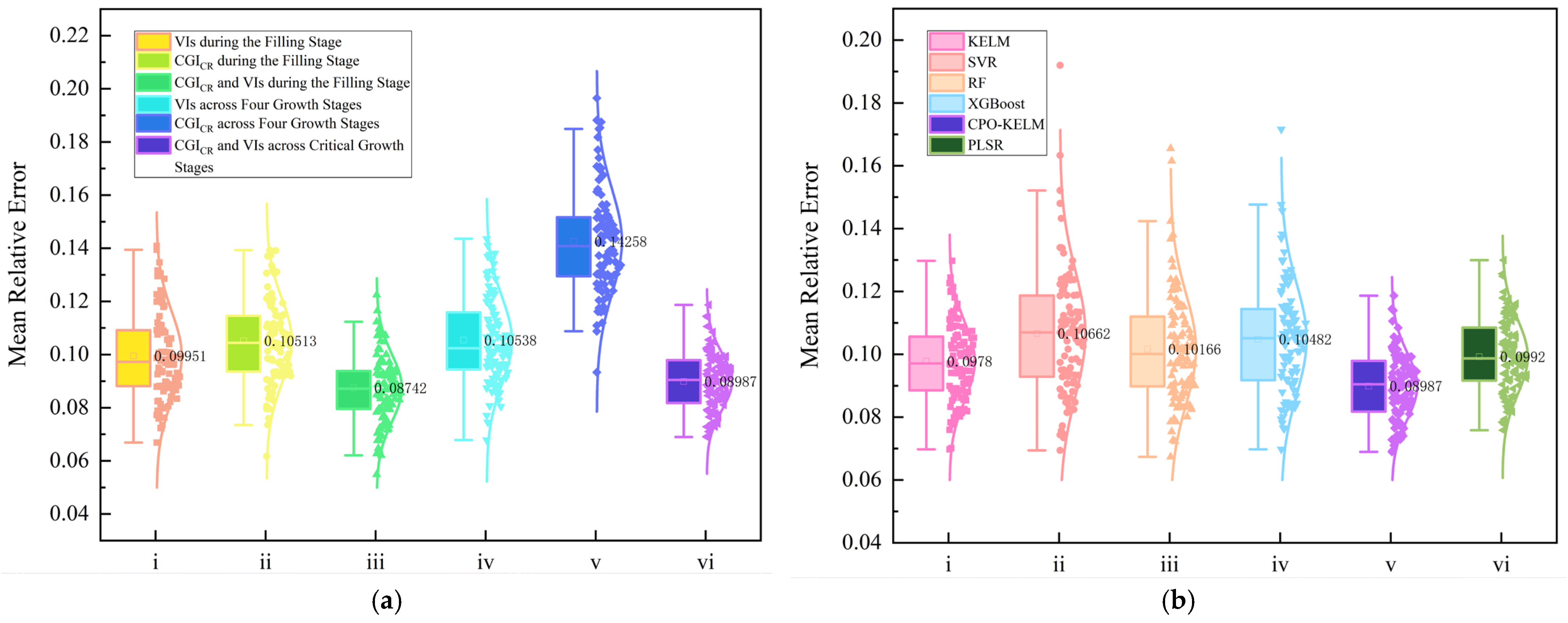
To further evaluate model stability under different data-partitioning conditions, 100 random data splits were performed for three types of models based on single-source data, multi-source feature fusion and multi-temporal image features, and MRE values were calculated. The results are shown in Figure 9, where Figure 9a presents a stability comparison of different feature combinations using the CPO-KELM algorithm and Figure 9b shows a stability comparison of different machine learning models that integrate CGI_CR with VIs from the heading and filling stages.

As shown in Figure 9a, the models based on VIs or CGI_CR during the filling period showed a relatively large fluctuation range in MRE values, whereas the model based on CGI_CR and VIs showed a relatively small fluctuation range, with a maximum value of approximately 0.11. This indicates that multi-source feature fusion provides greater stability than single-source approaches. Similarly, in the multi-temporal models, the CGI_CR-based model across the four growth stages exhibited a wider MRE variation range than the VI-based model across the same stages. The model integrating CGI_CR and VIs from the heading and filling stages showed the narrowest MRE range, varying from 6.8% to 11.8%, and the stability was the highest. The mean and median relative errors were relatively low at 9.04% and 8.99%, respectively. Despite their superior overall performance, the multi-temporal models exhibited slightly larger extreme MRE values than those based solely on the single-growth stage (filling stage).

As shown in Figure 9b, when CGI_CR and VIs from the heading and filling stages were used as inputs, differences in error distributions among machine learning models were observed. The SVR model exhibited the largest MRE variation, with a wide interquartile range and high-error outliers approaching 0.19, as well as the highest median value (approximately 10.66%). XGBoost and RF also showed relatively wide error distributions with outliers, with median values of approximately 10.48% and 10.17%, respectively. PLSR, as the simplest linear baseline, achieved a median MRE of approximately 9.92%. By contrast, the CPO-KELM model showed the smallest variation range, the most compact distribution, and the lowest median MRE (approximately 8.99%). Although PLSR exhibited a distribution width comparable to CPO-KELM, its median MRE was notably higher, confirming the stability advantage of CPO-KELM in handling high-dimensional features.

4. Discussion

4.1. Agronomic Rationale and Stage-Dependent Relationships Among CGI Components

Crop growth exhibits pronounced stage-specific characteristics, and single indicators are insufficient to capture variations in crop status across developmental stages. In addition, spectral saturation tends to occur after canopy closure [69,70]. Therefore, constructing a CGI to comprehensively characterise crop population traits is essential for improving the reliability of growth monitoring and yield assessment.

From the perspective of integrating agronomy and remote sensing, crop growth indicators include parameters reflecting population structural characteristics, such as LAI and stem tiller density; biophysical variables, such as AGB; and biochemical indicators, such as SPAD and nitrogen content. Different types of indicators exhibit distinct response characteristics during crop growth. Based on these considerations, stem tiller density, LAI and AGB were selected as the key variables in this study. These variables represent different aspects of crop growth, including population size, canopy structure and dry matter accumulation, respectively, thereby capturing the complementary dimensions of crop development [21,71,72]. Their agronomic relevance lies not only in the different crop traits they represent, but also in the way these traits are linked across successive developmental stages.

During the early growth period, stem tiller density contributes to crop population establishment and provides the basis for subsequent productive spike formation. Tiller development also contributes to leaf-area expansion; therefore, an appropriate tiller population favours canopy establishment and LAI development. However, excessive population density may intensify competition for light, water and nutrients, increase self-shading, and reduce tiller survival. Stem tiller density consequently influences yield formation through both the establishment of potential spike number and its effect on subsequent canopy structure. From jointing to heading, as the number of surviving tillers and productive spikes gradually stabilises, LAI increasingly reflects the capacity of the canopy to intercept radiation and produce assimilates. Canopy photosynthesis during this period supports stem elongation, spike development and the formation of yield components. Continued canopy assimilation also promotes AGB accumulation. AGB can therefore be regarded, in part, as the cumulative outcome of earlier population establishment and canopy photosynthetic activity. However, its contribution to final yield also depends on the subsequent allocation of dry matter to reproductive organs. By the filling stage, productive spike number is largely established, and the role of stem tiller density becomes relatively fixed. At this stage, LAI reflects the canopy leaf area available for continued radiation interception and photosynthesis, whereas AGB integrates the cumulative production and accumulation of dry matter. The maintenance of green leaf area supports post-anthesis photosynthesis, while part of the previously accumulated dry matter may be remobilised to developing kernels. Final yield therefore depends on the coordination among the assimilate demand of developing kernels, continued canopy assimilation and dry matter allocation. Consequently, high LAI or AGB alone does not necessarily result in high yield when canopy structure, reproductive capacity or dry matter partitioning is unfavourable.

Overall, stem tiller density, LAI and AGB provide complementary information on the progression from population establishment to canopy development, biomass accumulation and kernel filling. Their joint incorporation into the CGI captures both the individual information provided by each trait and their stage-dependent relationships during yield formation. Compared with single indicators, this integrated representation provides a more complete characterisation of wheat growth and enhances the responsiveness of the CGI to variations across growth stages [73]. The changing roles of these parameters throughout crop development also provide an agronomic basis for assigning stage-specific weights during CGI construction.

Other physiological and biochemical indicators, such as SPAD and nitrogen content, are valuable for characterising leaf chlorophyll status and crop nutritional conditions. However, their integration with VIs for yield estimation presents several limitations. These indicators primarily represent physiological conditions at the leaf scale, whereas VIs are derived from canopy-scale spectral reflectance, which may introduce uncertainties in model construction. Furthermore, after canopy closure, spectral saturation and variations in canopy structure may reduce the sensitivity of canopy reflectance to changes in leaf biochemical properties, thereby increasing uncertainty in the remote-sensing estimation of SPAD or nitrogen status. Therefore, within the remote sensing-based modelling framework of this study, prioritising stem tiller density, LAI and AGB, which characterise crop population establishment, canopy leaf-area status and aboveground dry matter accumulation, respectively, helps improve both model stability and interpretability for regional-scale yield prediction. The incorporation of physiological indicators such as SPAD and nitrogen content will be explored in future work to further improve the model.

4.2. Impact of Weighting Methods on CGI Construction

The relative importance of growth parameters varies throughout the crop growth cycle, making weight allocation a critical factor in constructing CGIs. Previous studies have indicated that conventional weighting approaches simplify this process but may fail to accurately represent the contribution of individual parameters to crop development [74]. In multi-indicator evaluation systems, weight allocation should account for both the information provided by individual indicators and the relationships among them. Therefore, two objective weighting methods, the CRITIC method and the coefficient of variation method, were applied to construct CGIs for wheat.

The CGI_CV assigns weights solely based on the degree of dispersion of each parameter, giving greater weight to those with higher variability to reflect the amount of information they contain. However, this method does not account for inter-parameter correlations and may amplify redundant information when multiple correlated variables are included. By contrast, the CRITIC method accounts for both the variability and the correlation structure across parameters. By incorporating correlation coefficients, it quantifies the relationships among indicators and identifies redundant information, thereby avoiding repeated contributions from highly correlated variables to the composite index. When parameters are strongly correlated, their information tends to overlap. In such cases, the CRITIC method assigns relatively lower weights to these variables, thereby reducing the influence of redundant information and preserving the independent contributions of each indicator. This characteristic is particularly important for crop growth parameters, which often exhibit strong correlations. For instance, stem tiller density and AGB frequently show high correlations at certain growth stages. By adjusting the weights of correlated variables, the CRITIC method mitigates redundancy and produces a more balanced and informative composite indicator.

In addition, the weight distribution varied across growth stages, reflecting stage-specific contributions of growth parameters. LAI maintained the highest weight from jointing to filling, ranging from 0.42 to 0.52, and showed a further upwards trend during the filling period. This underscores the dominant role of canopy photosynthetic area in sustaining yield potential during late growth stages. By contrast, during the early population establishment phase at the jointing stage, tiller density and AGB contributed nearly equally, with weights of approximately 0.29 each. Upon entering the filling stage, as spike number stabilises, the direct contribution of tiller density decreases markedly (with its weight declining to 0.22), whereas AGB (0.26), representing the dry matter available for grain filling, becomes relatively more important. This shift reflects the transition in wheat growth from population establishment to dry matter accumulation. At the same time, compared with the coefficient of variation approach, CRITIC showed a stronger ability to differentiate among individual parameter contributions, indicating that incorporating both variability and correlation provides a more effective representation of parameter contributions [36]. Further demonstrating that objective weighting methods considering both variability and inter-parameter relationships can improve model stability and interpretability. Moreover, combined with the correlation analysis and modelling results presented above, CGI_CR consistently outperformed CGI_CV across different growth stages. Therefore, subsequent analyses were primarily conducted based on CGI_CR.

4.3. Role of Multi-Source and Multi-Temporal Feature Fusion for Yield Estimation

Integration of multi-source and multi-temporal features significantly enhanced the wheat model performance. As shown in Table 8, the prediction accuracy of models based on single-growth stages increased progressively with crop development. Among them, the VI-based CPO-KELM model performed best during the filling stage, consistent with previous findings that canopy characteristics in later growth stages are more closely related to yield [27]. This indicates that features from later stages provide more direct representations of yield under single-stage conditions.

The introduction of multi-source features showed differentiated effects at different growth stages. It demonstrated certain performance improvements during the jointing, heading and filling stages, indicating that agronomic parameters and spectral information provide complementary information for characterising wheat canopies [75]. However, this improvement was less pronounced during the booting stage, indicating that different growth stages respond differently to the feature information. Furthermore, the model combining CGI_CR and VIs generally outperformed that based on CGI_CV, consistent with the findings from the weighting analysis. Recent studies have similarly demonstrated that combining multi-source remote-sensing, environmental and crop-trait data with deep learning models, such as CNN–BiLSTM and Transformer architectures, can improve wheat yield prediction by exploiting complementary and temporal information [76,77]. In contrast, the present study emphasises the agronomic interpretability of the composite growth indicator and identifies an informative heading–filling feature combination through correlation and ablation analyses.

Building on this, multi-temporal features further improved model performance. The model based on VIs from the four growth stages already enhanced prediction accuracy compared with single-stage models. When combined with CGI_CR features from the heading and filling stages, the model achieved its highest validation R² of 0.92, exceeding the best single-stage model at the filling stage (R² = 0.884). This result suggests that although observations at the filling stage can effectively reflect dry matter accumulation, they cannot fully represent the entire yield formation process.

Notably, although multi-temporal feature fusion generally enhanced model performance, not all growth stages contributed positively. The ablation experiment in the Cross-Stage Feature Redundancy Assessment and Ablation Results showed that removing the jointing and booting stages from the full four-stage model improved validation R². This counterintuitive result can be explained from two perspectives. First, the jointing and booting stages represent a transitional period from vegetative to reproductive growth, during which the relationships between canopy spectral/agronomic traits and final yield remain unstable and are susceptible to cultivar differences and field management practices—thus carrying considerable stage-specific noise rather than yield-relevant information. Second, when these highly correlated and noise-prone early-stage features are fed into the model together with the strongly predictive filling-stage features, the kernel matrix of the KELM may become ill-conditioned, preventing the CPO-optimised regularisation coefficient from converging to the global optimum and thereby impairing generalisation. These findings suggest that, in feature fusion, a larger feature set does not necessarily yield better performance; instead, features should be selected based on their actual contribution to yield formation, and redundant early-stage features with high noise levels should be excluded to improve both regularisation efficiency and estimation stability.

Because different growth stages contribute differently to yield, the heading stage primarily reflects yield-determining factors, such as ear density and potential grain count, while the filling stage mainly reflects the efficiency of transport and accumulation of photosynthetic products. Therefore, compared with simply aggregating features across all growth stages, selecting key stages for feature integration yields better predictive performance. The proposed multi-temporal model integrates information from the heading and filling stages, accounting for both yield formation and grain filling processes, and thus compensates for the temporal variations that single-phase models fail to capture in the later stages.

4.4. Comparison and Stability Analysis of Machine Learning Models

Various machine learning models exhibited distinct differences in wheat yield estimation. As indicated in Table 10, RF and XGBoost achieved high fitting accuracy on the training set (R² > 0.92), but their validation performance declined (R² = 0.802 and 0.792), with relatively high RMSE values, indicating a degree of instability under different data-partitioning conditions. RF is widely recognised for its generalisation ability and adaptability to high-dimensional data in remote sensing applications [78,79]. However, with multi-source and multi-temporal feature inputs, the dimensionality of input variables increases substantially, whereas the sample size remains relatively limited. This imbalance increases the vulnerability of the model to the complexity of the feature space and variations in sample distribution, thereby reducing its generalisation performance. Furthermore, spatial heterogeneity among different regions and imbalanced training sample distributions may also lead to variations in the model’s performance across different subsets [80,81]. In addition to these data-related factors, feature construction strategies also contribute to the instability of RF and XGBoost.

As demonstrated by the correlation analysis in the Cross-Stage Feature Redundancy Assessment and Ablation Results, more than half of the feature combinations have absolute correlation coefficients exceeding 0.70, indicating a certain degree of information redundancy in the multi-temporal feature space. When multiple highly correlated features are used simultaneously in decision tree splitting, RF and XGBoost tend to repeatedly utilise similar information across different branches, leading to structural complexity and unstable generalisation boundaries. This provides a partial explanation for their notable decline in validation R². Additionally, although multi-source feature fusion provides richer information [82], redundancy may exist among vegetation indices that capture similar canopy structural or chlorophyll-related characteristics and the inclusion of multi-temporal features further increases model complexity. Under such high-dimensional and highly correlated feature settings, greater demands are placed on model generalisation ability.

In comparison, the optimised CPO-KELM model demonstrated improved accuracy and stability. The introduction of PLSR as a linear benchmark indicated that non-linear mapping further improved the estimation accuracy (Section 3.6.2). The unoptimised KELM and SVR models achieved validation R² values of 0.823 and 0.809, respectively, with relatively large error fluctuations, indicating higher sensitivity to sample perturbations. After optimisation using CPO, the KELM model achieved a validation R² of 0.846, while reducing RMSE to 580.78 and increasing RPD to 2.568. The results from 100 repeated random runs further showed that the CPO-KELM model produced a more concentrated error distribution with fewer outliers (Figure 9b), demonstrating greater stability. This indicates that, when integrating information from different growth stages under the present multi-source and multi-temporal conditions, the model is less sensitive to perturbations in the training samples, thereby maintaining relatively consistent predictive performance under different data partitioning conditions. The computational efficiency also differed across models. The training time of the CPO-KELM model was only 0.002 s, substantially lower than that of RF and XGBoost. However, due to the relatively small dataset, the training time of all models falls within the millisecond range and the differences are not particularly meaningful for comparison. Therefore, a more informative evaluation should consider both the total runtime and predictive performance, under which the optimised method achieves a consistent balance between efficiency and reliability.

Overall, model performance is influenced not only by algorithm design but also by feature construction strategies. Comparisons among single-stage, multi-source and multi-temporal models show that integrating complementary information from multiple sources and growth stages improves both accuracy and robustness. Building on this advantage, the optimised CPO-KELM model demonstrates better stability and generalisation ability under the current multi-source and multi-temporal feature conditions. Compared with traditional models, which are more prone to overfitting or instability in high-dimensional feature settings, the proposed method maintains relatively consistent predictive performance under complex feature structures, thereby yielding more stable yield estimates.

4.5. Limitations and Future Perspectives

Independent test results indicate that the model still exhibits certain limitations in generalisation under cross-regional and multi-year conditions. Compared with the validation set, this dataset was collected at a different experimental site and in a different year and included different wheat cultivars and planting-density treatments, forming a relatively strict external test that simultaneously encompasses spatial, temporal, variety, and management differences. Owing to limitations in data collection, only the jointing stage was evaluated on the independent test set.

A comparison of the results in Table 4 with those from the original validation set (Figure 6) showed that overall prediction accuracy decreased, with RPD values of <2.0. This suggests that the model at the jointing stage is better suited to early risk screening than to final yield estimation. The broader yield range of the independent dataset may have partly contributed to the increased RMSE. Environmental differences between the two experimental sites may have affected crop growth and canopy spectral responses. Cultivar differences may have altered phenology, canopy structure and dry matter allocation, while variations in planting density and field management may have changed stem tiller density, LAI, AGB and their relationships with final yield. Differences in illumination, flight conditions, image calibration and other remote-sensing acquisition conditions may also have affected the comparability of reflectance data between the two datasets. Moreover, the relatively low R² observed during the jointing stage in the original validation results, compared with other growth stages, indicates that early-stage features contained less direct information on final yield. Consequently, the independent test results may better reflect both cross-site differences and the limited predictive ability of jointing-stage data. Nevertheless, integrating multi-source features (CGI_CR and VIs) partially alleviates uncertainties arising from environmental heterogeneity.

Based on the above external validation results, this study has several limitations. Although combining CGI_CR and VIs from multiple growth stages has enhanced prediction accuracy and stability to some extent, the model is mainly constructed based on key growth stages due to data constraints and its ability to represent the continuous crop growth process still needs further improvement. In addition, independent testing was mainly conducted at the jointing stage, and systematic validation across multiple growth stages and more complex regional conditions remains lacking, which limits a comprehensive evaluation of the model’s generalisation ability. A further practical limitation concerns the data acquisition strategy. The multi-temporal UAV flights and coincident field measurements of agronomic parameters are time-consuming and labour-intensive, which may hinder direct operational deployment over large areas.

The ablation results provide a basis for simplifying data collection strategies. Under the conditions of this study, the optimal feature combination did not require observations from all four growth stages, and excluding the jointing and booting stages did not reduce validation performance. Therefore, UAV observations and field measurements at the heading and filling stages may be prioritised when multi-stage data acquisition is feasible. When field resources or UAV flight opportunities are limited, using only filling stage data can serve as a cost-effective alternative.

Future studies could improve the representation of crop growth dynamics by incorporating remote sensing data with higher temporal resolution and by adopting modelling approaches capable of capturing temporal dependencies, such as recurrent neural networks or Transformer-based models. Simultaneously, integrating multi-source environmental data, including soil moisture and meteorological variables, and exploring transfer learning methods may enhance the model’s adaptability under different regional and climatic conditions. Remote-sensing-based or automated estimation of stem tiller density, LAI and AGB could also reduce dependence on manual field measurements and improve operational scalability. Moreover, validation using larger, multi-year, cross-regional datasets or independent multi-regional data will be essential for further assessing model robustness and applicability.

5. Conclusions

This study integrated UAV multi-spectral data with agronomic parameters to develop a winter wheat yield estimation model based on the fusion of multi-temporal CGI_CR and VIs, achieving the highest internal validation performance (R² = 0.920). These results indicate that integrating complementary spectral and agronomic information from multiple growth stages improved yield estimation compared with single-source or single-stage modelling. Correlation and ablation analyses further showed that the contributions of different growth stages were unequal and that selecting informative growth stages was more effective than simply combining all available temporal features. The CGI_CR used in the model incorporated the structural parameter of stem tiller density and reduced redundancy among variables through differential weighting, enabling key growth information to be captured more effectively during modelling and resulting in a superior performance to that of single-source models. In model comparison experiments, the CPO-KELM model outperformed the non-optimised KELM and the evaluated baseline models, including SVR, RF, XGBoost and PLSR, supporting its suitability for modelling the nonlinear relationships between multi-source, multi-temporal features and winter wheat yield. From a practical perspective, these findings provide a basis for prioritising informative growth stages during UAV and field-data acquisition, which may reduce unnecessary observations and support pre-harvest yield forecasting and precision field management. However, limitations remain regarding early-growth-stage prediction and cross-regional applications, as the independent validation dataset was only collected at the jointing stage. Future research should establish multi-stage, multi-year and multi-regional external validation datasets and incorporate environmental factors, including climate and soil conditions, to further enhance predictive reliability and adaptability across different regions and growth stages.

References

1. Men, X.; Dong, Z.; Li, L.; Yang, Q.; Zhang, Q.; Ou, F.; Lu, Z.; Li, C.; Yu, Y.; Zhuang, Q. Advances in the integrated management of wheat pests based on ecological regulation. Chin. J. Appl. Entomol. 2020, 57, 59–69. [Google Scholar] [CrossRef]
2. Chen, S.; Zhang, S.; Zhao, Z. Wheat yield prediction based on multi-source heterogeneous data and attention gate mechanism. J. Shandong Agric. Univ. Nat. Sci. Ed. 2024, 55, 444–452. [Google Scholar] [CrossRef]
3. Zeng, J.; Li, Y.; Wei, L.; Zhao, X.; Zhou, H. Application of random forest optimized neural network algorithm in winter wheat yield prediction: A survey. Intell. Comput. Appl. 2024, 14, 166–171. [Google Scholar] [CrossRef]
4. Sun, H.; Ma, J.; Wang, L. Changes in per capita wheat production in China in the context of climate change and population growth. Food Secur. 2023, 15, 597–612. [Google Scholar] [CrossRef] [Scilit] [PubMed]
5. Haseeb, M.; Tahir, Z.; Mahmood, S.A.; Tariq, A. Winter wheat yield prediction using linear and nonlinear machine learning algorithms based on climatological and remote sensing data. Inf. Process. Agric. 2025, 12, 431–444. [Google Scholar] [CrossRef] [Scilit]
6. Tan, X.; Zhang, J.; Wang, Z.; Chen, J.; Yang, F.; Yang, W. Prediction of maize yield in relay strip intercropping under different water and nitrogen conditions based on PLS. Sci. Agric. Sin. 2022, 55, 1127–1138. [Google Scholar] [CrossRef]
7. Mokhtari, A.; Yang, H.; Croft, H.; Luca, S.V.; Li, F.; Minceva, M.; Schmidthalter, U.; Yu, K. Satellite-based winter wheat yield estimation with a newly parameterized LUE model based on crop water status and leaf chlorophyll content. Field Crops Res. 2025, 333, 110106. [Google Scholar] [CrossRef] [Scilit]
8. Hu, T.; Zhao, L.; Cui, X.; Zhang, J.; Li, X.; Wang, X. Reliability analysis of UAV multispectral data and estimation of winter wheat yield. Trans. Chin. Soc. Agric. Mach. 2023, 54, 217–225. [Google Scholar]
9. Zhao, S.; Wang, G.; Hu, L.; Xu, H.; Qu, D.; Lan, Y. Estimation of cotton growth parameters and yield based on UAV multi-spectral remote sensing. J. Chin. Agric. Mech. 2024, 45, 227–234. [Google Scholar] [CrossRef]
10. Han, W.; Peng, X.; Zhang, L.; Niu, Y. Summer maize yield estimation based on vegetation index derived from multi-temporal UAV remote sensing. Trans. Chin. Soc. Agric. Mach. 2020, 51, 148–155. [Google Scholar] [CrossRef]
11. Li, Z.; Li, L.; Chen, Z.; Cheng, Q.; Xu, H.; Pang, C. Estimating winter wheat yield using UAV remote sensing imageries and stacking method. J. Irrig. Drain. 2021, 40, 50–56. [Google Scholar] [CrossRef]
12. Wan, L.; Cen, H.; Zhu, J.; Zhang, J.; Zhu, Y.; Sun, D.; Du, X.; Li, Z.; Weng, H.; Li, X.; et al. Grain yield prediction of rice using multi-temporal UAV-based RGB and multispectral images and model transfer—A case study of small farmlands in the south of China. Agric. For. Meteorol. 2020, 291, 108096. [Google Scholar] [CrossRef] [Scilit]
13. Ma, C.; Liu, M.; Ding, F.; Li, C.; Cui, Y.; Chen, W.; Wang, Y. Wheat growth monitoring and yield estimation based on remote sensing data assimilation into the SAFY crop growth model. Sci. Rep. 2022, 12, 5473. [Google Scholar] [CrossRef] [Scilit] [PubMed]
14. Wu, Y.; Xiong, Y.; Yu, W.; Gu, Y.; Zheng, H.; Jiang, C.; Yao, X.; Zhu, Y.; Cao, W.; Cheng, T. In-season estimation of aboveground biomass and yield in winter wheat with a UAV-based LUE model and machine learning. Plant Phenomics 2025, 8, 100162. [Google Scholar] [CrossRef] [Scilit] [PubMed]
15. Zhu, J.; Li, Y.; Wang, C.; Liu, P.; Lan, Y. Method for monitoring wheat growth status and estimating yield based on UAV multispectral remote sensing. Agronomy 2024, 14, 991. [Google Scholar] [CrossRef] [Scilit]
16. Ali, A.M.; Ibrahim, S.M.; Singh, B.J. Wheat grain yield and nitrogen uptake prediction using atLeaf and GreenSeeker portable optical sensors at jointing growth stage. Inf. Process. Agric. 2020, 7, 375–383. [Google Scholar] [CrossRef] [Scilit]
17. Wang, W.; Zhang, J.; Wang, H.; Cao, Q.; Tian, Y.; Zhu, Y.; Cao, W.; Liu, X. Non-destructive monitoring of rice growth key indicators based on fixed-wing UAV multispectral images. Sci. Agric. Sin. 2023, 56, 4175–4191. [Google Scholar] [CrossRef]
18. Ma, M.; Zhao, J.; Yang, T.; Liu, F.; Yuan, Y.; Ma, S.; Chang, Z. Estimating comprehensive growth index for drip-irrigated spring maize in Junggar Basin via satellite imagery and machine learning. Agric. Water Manag. 2025, 318, 109651. [Google Scholar] [CrossRef] [Scilit]
19. Wang, H.; Yao, Q.; Zhang, Z.; Qin, S.; Ma, L.; Lv, X.; Zhang, L. Comprehensive growth monitoring index using Sentinel-2A data for large-scale cotton production. Field Crops Res. 2024, 317, 109525. [Google Scholar] [CrossRef] [Scilit]
20. Du, M.; Ali, R.; Liu, Y. Inversion of wheat tiller density based on visible-band images of drone. Spectrosc. Spectr. Anal. 2021, 41, 3828–3836. [Google Scholar]
21. Hu, J.; Zhang, B.; Peng, D.; Yu, R.; Liu, Y.; Xiao, C.; Li, C.; Dong, T.; Fang, M.; Ye, H.; et al. Estimation of wheat tiller density using remote sensing data and machine learning methods. Front. Plant Sci. 2022, 13, 1075856. [Google Scholar] [CrossRef] [Scilit] [PubMed]
22. Parker, G.G. Tamm review: Leaf area index (LAI) is both a determinant and a consequence of important processes in vegetation canopies. For. Ecol. Manag. 2020, 477, 118496. [Google Scholar] [CrossRef] [Scilit]
23. Pei, H.; Feng, H.; Li, C.; Jin, X.; Li, Z.; Yang, G. Remote sensing monitoring of winter wheat growth with UAV based on comprehensive growth index. Trans. Chin. Soc. Agric. Eng. 2017, 33, 74–82. [Google Scholar] [CrossRef]
24. Ma, S.; Zhang, Z.; Zhang, J.; Luo, X.; Gao, R.; Ren, J.; Hou, X. Remote sensing monitoring of winter wheat growth using physico-chemical composite parameter and neural network. Trans. Chin. Soc. Agric. Eng. 2024, 40, 91–99. [Google Scholar] [CrossRef]
25. Wang, J.; Wang, P.; Tian, H.; Tansey, K.; Liu, J.; Quan, W. A deep learning framework combining CNN and GRU for improving wheat yield estimates using time series remotely sensed multi-variables. Comput. Electron. Agric. 2023, 206, 107705. [Google Scholar] [CrossRef] [Scilit]
26. Elsayed, S.; Elhoweity, M.; Ibrahim, H.H.; Dewir, Y.H.; Migdadi, H.M.; Schmidhalter, U. Thermal imaging and passive reflectance sensing to estimate the water status and grain yield of wheat under different irrigation regimes. Agric. Water Manag. 2017, 189, 98–110. [Google Scholar] [CrossRef] [Scilit]
27. Cheng, Q.; Xu, H.; Cao, Y.; Duan, F.; Chen, Z. Grain yield prediction of winter wheat using multi-temporal UAV based on multispectral vegetation index. Trans. Chin. Soc. Agric. Mach. 2021, 52, 160–167. [Google Scholar] [CrossRef]
28. Tian, T.; Zhang, Q.; Zhang, H.; He, Q.; Ji, F.; Zhu, L. Estimating yield of rice based on remote sensing by unmanned aerial vehicle. China Rice 2022, 28, 67–71. [Google Scholar] [CrossRef]
29. Li, X. Research on Wheat Growth Monitoring and Yield Estimation Based on UAV Remote Sensing. Master’s Thesis, Henan University of Science and Technology, Luoyang, China, 2024. [Google Scholar]
30. Liang, D.; Wang, C.; Liu, D.; Shi, X.; Feng, G.; Wang, J. A new high-quality strong-gluten spring wheat variety—Jin Qiang 11. J. Triticeae Crops 2019, 39, 91–93. [Google Scholar]
31. Wang, C.; Liang, D.; Wang, J.; Liu, D.; Pan, H.; Liu, J. Selection and cultivation techniques of a new high-quality strong-gluten spring wheat variety—Jin Qiang 9. Cereal Crop Res. 2016, 9, 221–222. [Google Scholar]
32. Yuan, J.; Yang, W. A high-yield and widely adaptable high-quality spring wheat variety—Longchun 23. J. Triticeae Crops 2009, 29, 740. [Google Scholar]
33. Zhou, W.; Li, W.; Li, H.; Zhang, S.; Shao, Q.; Zhu, S.; Wang, J.; Yan, S. Effects of planting density on starch quality in wheat grains and lodging resistance of stems. Jiangsu Agric. Sci. 2024, 52, 108–114. [Google Scholar] [CrossRef]
34. Lancashire, P.; Bleiholder, H.; Boom, T.; Langelüddeke, P.; Stauß, R.; Weber, E.; Witzenberger, A. A uniform decimal code for growth stages of crops and weeds. Ann. Appl. Biol. 1991, 119, 561–601. [Google Scholar] [CrossRef] [Scilit]
35. Brewer, K.; Clulow, A.; Sibanda, M.; Gokool, S.; Naiken, V.; Mabhaudhi, T. Predicting the chlorophyll content of maize over phenotyping as a proxy for crop health in smallholder farming systems. Remote Sens. 2022, 14, 518. [Google Scholar] [CrossRef] [Scilit]
36. Krishnan, A.R.; Kasim, M.M.; Hamid, R.; Ghazali, M.F. A modified CRITIC method to estimate the objective weights of decision criteria. Symmetry 2021, 13, 973. [Google Scholar] [CrossRef] [Scilit]
37. Tao, Z.; Ge, L.; Chen, H. Non-negative variable weight combination forecasting method based on sliding window. Control Decis. 2020, 35, 1446–1452. [Google Scholar] [CrossRef]
38. Li, F.; Li, D.; Elsayed, S.; Hu, Y.; Schmidhalter, U. Using optimized three-band spectral indices to assess canopy N uptake in corn and wheat. Eur. J. Agron. 2021, 127, 126286. [Google Scholar] [CrossRef] [Scilit]
39. Zhou, Q.; Wang, J.; Huo, Z.; Liu, C.; Wang, W.; Ding, L. Estimation of SPAD values in wheat canopy at different growth stages using UAV multispectral remote sensing. Spectrosc. Spectr. Anal. 2023, 43, 1912–1920. [Google Scholar]
40. Kataoka, T.; Kaneko, T.; Okamoto, H.; Hata, S. Crop growth estimation system using machine vision. In Proceedings of the 2003 IEEE/ASME International Conference on Advanced Intelligent Mechatronics, Kobe, Japan, 20–24 July 2003. [Google Scholar]
41. Gitelson, A.A.; Vina, A.; Arkebauer, T.J.; Rundquist, D.C.; Keydan, G.; Leavitt, B. Remote estimation of leaf area index and green leaf biomass in maize canopies. Geophys. Res. Lett. 2003, 30, 1248. [Google Scholar] [CrossRef] [Scilit]
42. Datt, B. A new reflectance index for remote sensing of chlorophyll content in higher plants: Tests using eucalyptus leaves. J. Plant Physiol. 1999, 154, 30–36. [Google Scholar] [CrossRef] [Scilit]
43. Richardson, A.J.; Everitt, J.H. Using spectral vegetation indices to estimate rangeland productivity. Geocarto Int. 1992, 7, 63–69. [Google Scholar] [CrossRef] [Scilit]
44. Rasmussen, J.; Ntakos, G.; Nielsen, J.; Svensgaard, J.; Poulsen, R.N.; Christensen, S. Are vegetation indices derived from consumer-grade cameras mounted on UAVs sufficiently reliable for assessing experimental plots? Eur. J. Agron. 2016, 74, 75–92. [Google Scholar] [CrossRef] [Scilit]
45. Huete, A.; Didan, K.; Miura, T.; Rodriguez, E.P.; Gao, X.; Ferreira, L.G. Overview of the radiometric and biophysical performance of the MODIS vegetation indices. Remote Sens. Environ. 2002, 83, 195–213. [Google Scholar] [CrossRef] [Scilit]
46. Jiang, Z.; Huete, A.R.; Didan, K.; Miura, T. Development of a two-band enhanced vegetation index without a blue band. Remote Sens. Environ. 2008, 112, 3833–3845. [Google Scholar] [CrossRef] [Scilit]
47. Woebbecke, D.M.; Meyer, G.E.; Von Bargen, K.; Mortensen, D.A. Color indices for weed identification under various soil, residue, and lighting conditions. Trans. ASAE 1995, 38, 259–269. [Google Scholar] [CrossRef] [Scilit]
48. Louhaichi, M.; Borman, M.M.; Johnson, D.E. Spatially located platform and aerial photography for documentation of grazing impacts on wheat. Geocarto Int. 2001, 16, 65–70. [Google Scholar] [CrossRef] [Scilit]
49. Gitelson, A.A.; Kaufman, Y.J.; Merzlyak, M.N. Use of a green channel in remote sensing of global vegetation from EOS-MODIS. Remote Sens. Environ. 1996, 58, 289–298. [Google Scholar] [CrossRef] [Scilit]
50. Buschmann, C.; Nagel, E. In vivo spectroscopy and internal optics of leaves as basis for remote sensing of vegetation. Int. J. Remote Sens. 1993, 14, 711–722. [Google Scholar] [CrossRef] [Scilit]
51. Sripada, R.P.; Heiniger, R.W.; White, J.G.; Meijer, A.D. Aerial color infrared photography for determining early in-season nitrogen requirements in corn. Agron. J. 2006, 98, 968–977. [Google Scholar] [CrossRef] [Scilit]
52. Haboudane, D.; Miller, J.R.; Pattey, E.; Zarco-Tejada, P.J.; Strachan, I.B. Hyperspectral vegetation indices and novel algorithms for predicting green LAI of crop canopies: Modeling and validation in the context of precision agriculture. Remote Sens. Environ. 2004, 90, 337–352. [Google Scholar] [CrossRef] [Scilit]
53. Han, Y.; Tang, R.; Liao, Z.; Zhai, B.; Fan, J. A novel hybrid GOA-XGB model for estimating wheat aboveground biomass using UAV-based multispectral vegetation indices. Remote Sens. 2022, 14, 3506. [Google Scholar] [CrossRef] [Scilit]
54. Lu, J.; Miao, Y.; Shi, W.; Li, J.; Yuan, F. Evaluating different approaches to non-destructive nitrogen status diagnosis of rice using portable RapidSCAN active canopy sensor. Sci. Rep. 2017, 7, 14073. [Google Scholar] [CrossRef] [Scilit] [PubMed]
55. Gong, P.; Pu, R.; Biging, G.S.; Larrieu, M.R. Estimation of forest leaf area index using vegetation indices derived from Hyperion hyperspectral data. IEEE Trans. Geosci. Remote Sens. 2003, 41, 1355–1362. [Google Scholar] [CrossRef] [Scilit]
56. Dash, J.; Curran, P.J. Evaluation of the MERIS terrestrial chlorophyll index (MTCI). Adv. Space Res. 2007, 39, 100–104. [Google Scholar] [CrossRef] [Scilit]
57. Goel, N.S.; Qin, W. Influences of canopy architecture on relationships between various vegetation indices and LAI and FPAR: A computer simulation. Remote Sens. Rev. 1994, 10, 309–347. [Google Scholar] [CrossRef] [Scilit]
58. Rondeaux, G.; Steven, M.; Baret, F. Optimization of soil-adjusted vegetation indices. Remote Sens. Environ. 1996, 55, 95–107. [Google Scholar] [CrossRef] [Scilit]
59. Chen, P.; Tremblay, N.; Wang, J.; Vigneault, P.; Huang, W.; Li, B. New index for crop canopy fresh biomass estimation. Spectrosc. Spectr. Anal. 2010, 30, 512–517. [Google Scholar] [CrossRef]
60. Pearson, R.L.; Miller, L.D. Remote mapping of standing crop biomass for estimation of the productivity of the shortgrass prairie. In Proceedings of the Eighth International Symposium on Remote Sensing of Environment, Ann Arbor, MI, USA, 2–6 October 1972. [Google Scholar]
61. Huete, A.R. A soil-adjusted vegetation index (SAVI). Remote Sens. Environ. 1988, 25, 295–309. [Google Scholar] [CrossRef] [Scilit]
62. Anchal, S.; Bahuguna, S.; Priti; Pal, P.K.; Kumar, D.; Murthy, P.V.S.; Kumar, A. Non-destructive method of biomass and nitrogen (N) level estimation in stevia rebaudiana using various multispectral indices. Geocarto Int. 2022, 37, 6409–6421. [Google Scholar] [CrossRef] [Scilit]
63. Xu, R.; Liang, X.; Qi, J.; Li, Z.; Zhang, S. Advances and trends in extreme learning machine. Chin. J. Comput. 2019, 42, 1640–1670. [Google Scholar] [CrossRef]
64. Afzal, A.L.; Nair, N.K.; Asharaf, S. Deep kernel learning in extreme learning machines. Pattern Anal. Appl. 2020, 24, 11–19. [Google Scholar] [CrossRef] [Scilit]
65. Huang, G.; Zhou, H.; Ding, X.; Zhang, R. Extreme learning machine for regression and multiclass classification. IEEE Trans. Syst. Man Cybern. B 2012, 42, 513–529. [Google Scholar] [CrossRef] [Scilit] [PubMed]
66. Abdel-Basset, M.; Mohamed, R.; Abouhawwash, M. Crested porcupine optimizer: A new nature-inspired metaheuristic. Knowl.-Based Syst. 2024, 284, 111257. [Google Scholar] [CrossRef] [Scilit]
67. Chen, H.; Xu, T.; Huang, Y.; Xin, D.; Zhong, C. MCPSFOA: Multi-strategy enhanced crested porcupine-starfish optimization algorithm for global optimization and engineering design. Comput. Model. Eng. Sci. 2026, 146, 16. [Google Scholar] [CrossRef] [Scilit]
68. Dong, T.; Liu, J.; Qian, B.; He, L.; Liu, J.; Wang, R.; Jing, Q.; Champagne, C.; McNairn, H.; Powers, J.; et al. Estimating crop biomass using leaf area index derived from Landsat 8 and Sentinel-2 data. ISPRS J. Photogramm. Remote Sens. 2020, 168, 236–250. [Google Scholar] [CrossRef] [Scilit]
69. Liu, Y.; Feng, H.; Fan, Y.; Yue, J.; Yang, F.; Fan, J.; Ma, Y.; Chen, R.; Bian, M.; Yang, G. Utilizing UAV-based hyperspectral remote sensing combined with various agronomic traits to monitor potato growth and estimate yield. Comput. Electron. Agric. 2025, 231, 109984. [Google Scholar] [CrossRef] [Scilit]
70. Tian, Z.; Fan, J.; Yu, T.; Leom, N.D.; Kaeppler, S.M.; Zhang, Z. Mitigating NDVI saturation in imagery of dense and healthy vegetation. ISPRS J. Photogramm. Remote Sens. 2025, 227, 234–250. [Google Scholar] [CrossRef] [Scilit]
71. Peng, Y.; Zhu, T.; Li, Y.; Dai, C.; Fang, S.; Gong, Y.; Wu, X.; Zhu, R.; Liu, K. Remote prediction of yield based on LAI estimation in oilseed rape under different planting methods and nitrogen fertilizer applications. Agric. For. Meteorol. 2019, 271, 116–125. [Google Scholar] [CrossRef] [Scilit]
72. Feng, H.; Fan, Y.; Yue, J.; Bian, M.; Liu, Y.; Chen, R.; Ma, Y.; Fan, J.; Yang, G.; Zhao, C. Estimation of potato above-ground biomass based on the VGC-AGB model and deep learning. Comput. Electron. Agric. 2025, 232, 110122. [Google Scholar] [CrossRef] [Scilit]
73. Zhai, L.; Wei, F.; Feng, H.; Li, C.; Yang, G. Monitoring winter wheat growth using comprehensive indicators. Jiangsu Agric. Sci. 2020, 48, 244–249. [Google Scholar] [CrossRef]
74. Xu, Y.; Cheng, Q.; Wei, X.; Yang, B.; Xia, S.; Rui, T.; Zhang, S. Monitoring of winter wheat growth under UAV using variation coefficient method and optimized neural network. Trans. Chin. Soc. Agric. Eng. 2021, 37, 71–80. [Google Scholar] [CrossRef]
75. Gracia-Romero, A.; Rufo, R.; Gómez-Candón, D.; Soriano, J.M.; Bellvert, J.; Yannam, V.R.R.; Gulino, D.; Lopes, M.S. Improving in-season wheat yield prediction using remote sensing and additional agronomic traits as predictors. Front. Plant Sci. 2023, 14, 1063983. [Google Scholar] [CrossRef] [Scilit] [PubMed]
76. Zhang, L.; Li, C.; Wu, X.; Xiang, H.; Jiao, Y.; Chai, H. BO-CNN-BiLSTM deep learning model integrating multisource remote sensing data for improving winter wheat yield estimation. Front. Plant Sci. 2024, 15, 1500499. [Google Scholar] [CrossRef] [Scilit] [PubMed]
77. Ge, Y.; Zhu, Z.; Jin, S.; Zang, J.; Zhang, R.; Li, Q.; Sun, Z.; Liu, S.; Xu, H.; Zhai, Z. Winter wheat yield prediction using UAV-based multivariate time series data and variate-independent tokenization. Plant Phenomics 2025, 7, 100039. [Google Scholar] [CrossRef] [Scilit] [PubMed]
78. Belgiu, M.; Drăguţ, L. Random forest in remote sensing: A review of applications and future directions. ISPRS J. Photogramm. Remote Sens. 2016, 114, 24–31. [Google Scholar] [CrossRef] [Scilit]
79. Jabed, M.A.; Murad, M.A.A. Crop yield prediction in agriculture: A comprehensive review of machine learning and deep learning approaches, with insights for future research and sustainability. Heliyon 2024, 10, e40836. [Google Scholar] [CrossRef] [Scilit] [PubMed]
80. Colditz, R.R. An evaluation of different training sample allocation schemes for discrete and continuous land cover classification using decision tree-based algorithms. Remote Sens. 2015, 7, 9655–9681. [Google Scholar] [CrossRef] [Scilit]
81. Mellor, A.; Boukir, S.; Haywood, A.; Jones, S. Exploring issues of training data imbalance and mislabelling on random forest performance for large area land cover classification using the ensemble margin. ISPRS J. Photogramm. Remote Sens. 2015, 105, 155–168. [Google Scholar] [CrossRef] [Scilit]
82. Corcoran, J.M.; Knight, J.F.; Gallant, A.L. Influence of multi-source and multi-temporal remotely sensed and ancillary data on the accuracy of random forest classification of wetlands in Northern Minnesota. Remote Sens. 2013, 5, 3212–3238. [Google Scholar] [CrossRef] [Scilit]
Figure 1. Map showing the location of the intelligent agriculture demonstration farm of China’s first tractor company.
Agronomy 16 01419 g001
Figure 2. Distribution of field trials in small plots.
Agronomy 16 01419 g002
Figure 3. Examples of pre-processed images. (a) Original image. (b) Grayscale mask image. (c) ROI after removing background. The square in (c) indicates one of the 81 plot-level ROIs.
Agronomy 16 01419 g003
Figure 4. SHAP value analysis of VIs at different growth stages. Each point represents an individual sample; red hues correspond to high vegetation indices, and blue hues indicate low values. When the distribution of samples is far from the SHAP value of 0, the influence of this index on the model prediction is strong. The figure displays only the top 10 ranked VIs.
Agronomy 16 01419 g004
Figure 5. Temporal variations in Pearson correlation coefficients (r) between individual agronomic parameters (tiller density, LAI, and AGB) and final grain yield across four major growth stages. ** indicate extremely significant correlations.
Agronomy 16 01419 g005
Figure 6. Performance of the single-temporal yield estimation model. (a) Yield estimation based on VIs. (b) Yield estimation based on CGICR. (c) Yield estimation based on CGICV and VIs. (d) Yield estimation based on CGICR and VIs.
Agronomy 16 01419 g006
Figure 7. Yield estimation model based on multiple growth stages. Relationship between the predicted and actual values of the multi-temporal yield estimation model based on (a) VIs, (b) CGIs and (c) a combination of CGIs and VIs.
Agronomy 16 01419 g007
Figure 8. Pearson correlation matrix of the 20 multi-temporal features. The upper triangle shows correlation coefficients; bubble sizes in the lower triangle are proportional to |r|. Black squares delineate the 5 × 5 blocks corresponding to each growth stage.
Agronomy 16 01419 g008
Figure 9. Stability analysis of different wheat yield estimation models. (a) Stability comparison of different feature combinations using the CPO-KELM algorithm. (b) Stability comparison of different machine learning models using VIs and CGICR from two growth stages.
Agronomy 16 01419 g009