A Short-Term Yield Prediction Method for Greenhouse Strawberries Integrating Visual Phenology and Meteorological Sequences

Abstract

Highly perishable strawberries demand strict post-harvest time management, making accurate short-term yield prediction central to optimizing modern greenhouse production and supply chain scheduling. However, existing models that rely excessively on isolated environmental factors exhibit delayed responsiveness to actual crop physiological dynamics and struggle with integrating multimodal data. To overcome these limitations, we propose a short-term method for predicting greenhouse strawberry yield that integrates visual phenology with meteorological sequences. The proposed method was validated using a multimodal dataset acquired from 150 tracked greenhouse strawberry plants over a 72-day monitoring period (11 December 2025, to 20 February 2026), incorporating continuous microclimate records and an image repository of 784 original images annotated into five distinct phenological classes (flower, green, white, pink, and red). First, using our improved YOLO11-SC model, we effectively resolve challenges of complex illumination and dense foliage occlusion, achieving high-precision automated extraction of five consecutive strawberry phenological stages. Second, by fusing these visual markers with meteorological time series (e.g., temperature, humidity, and light intensity), we construct a multimodal spatiotemporal feature matrix. To accommodate diverse smart agriculture application scenarios, we designed two distinct prediction architectures: on servers with ample computing power, a Bidirectional Temporal Convolutional Network with self-attention (BiTCN-SA) to achieve highly accurate predictions; and for resource-constrained IoT edge nodes, a lightweight machine learning ensemble (Stack-LGR). Experimental results demonstrate that, in predicting the cumulative mature fruit yield within the next harvesting cycle, BiTCN-SA achieves strong performance with a coefficient of determination ($R^2$) of 0.958 and a root mean square error (RMSE) of 3.154. Simultaneously, the edge-deployed Stack-LGR ensemble maintains stable prediction accuracy ($R^2$ = 0.892) while ensuring acceptable inference latency. This study mitigates the latency limitations of single-environment-driven models. It provides a solution for precise crop yield prediction and tiered computational deployment, with good predictive performance, deployment adaptability, and methodological reference value.

1. Introduction

Strawberries, as one of the world’s most economically valuable horticultural crops, are widely favored by consumers for their unique flavor, vibrant color, and rich nutritional value [1]. With the rapid development of protected agriculture, strawberry production has shifted toward an intensive model characterized by high inputs and outputs, occupying a pivotal position in the modern agricultural economy [2]. However, strawberries are typically highly perishable agricultural products with an extremely short post-harvest shelf life, and market prices are highly sensitive to yield fluctuations. Therefore, achieving high-precision short-term yield prediction is not only a technical challenge involving the integration of multi-source heterogeneous data but also a core driver enabling the strawberry industry to precisely allocate production factors, efficiently manage supply chain turnover, and maximize economic benefits. Despite this urgency, traditional yield prediction primarily relies on manual field sampling, a method that lags significantly in large-scale greenhouse cultivation. Manual sampling is not only labor-intensive and costly but is also highly susceptible to observer bias, leading to inevitable random errors in the prediction results [3]. This makes it difficult to meet the requirements of real-time data and objectivity demanded by modern smart agriculture.

To overcome the numerous limitations of manual sampling, researchers in the early exploratory stages of crop yield prediction turned to statistical methods based on objective environmental data. Such studies primarily focused on identifying correlations between meteorological variables (such as temperature, precipitation, relative humidity, and solar radiation) and final yield. For instance, in studies involving specific cash crops such as strawberries, researchers utilized Pearson’s correlation analysis and multiple linear regression to thoroughly evaluate the statistical impacts of key weather indicators at different growth stages on flowering and fruiting phenology, as well as final yield [4,5]. As research progressed, models such as principal component regression (PCR) and partial least squares (PLSs) regression were introduced into agricultural modeling to address the multicollinearity inherent in high-dimensional meteorological features. These methods significantly enhance the stability of predictive models by extracting mutually independent principal components for yield fitting, particularly when sample sizes are limited [6,7]. Furthermore, given the cyclical fluctuations in harvesting cycles, time-series and spatial statistical models, such as the Autoregressive Integrated Moving Average (ARIMA) model, have been widely applied to process historical lagged data for predicting short-term yield trends [8]. Despite these advancements, traditional statistical models still exhibit inherent limitations in practical applications. They typically focus on fitting relatively simple linear relationships and often struggle to model the highly nonlinear, complex microclimatic interactions found in modern facility agriculture. More importantly, such macro-level models fail to incorporate direct observations of crop phenotypic traits (such as the number of flowers and fruits, or canopy architecture), making it difficult to achieve precise predictions.

To overcome the limitations of traditional statistical models in handling complex nonlinear agricultural data, researchers have increasingly turned to machine learning (ML) and deep learning (DL) technologies. Unlike traditional regression analysis, which relies on strict statistical assumptions, ML algorithms, with their superior pattern recognition and nonlinear mapping capabilities, offer a new paradigm for breaking through the accuracy bottlenecks in traditional yield prediction [9]. In analyzing complex environmental response mechanisms, Borrero et al. [10] noted that hybrid models based on nonlinear autoregression and support vector regression (SVR) can effectively reconstruct the nonlinear mapping relationships between multi-source drivers and berry yield, thereby significantly enhancing the stability of short-term yield estimation. Furthermore, Oliveira et al. [11] utilized algorithms such as Support Vector Machines (SVMs) to process Unmanned Aerial Vehicle (UAV) multispectral data, demonstrating that ML models significantly outperform traditional linear methods in estimating key phenotypic parameters such as fruit weight and leaf count. In handling high-dimensional factors, ensemble learning algorithms such as XGBoost and Random Forest have been widely demonstrated to possess extremely high explanatory power ($R^2>0.82$) when analyzing the complex interactions between meteorological factors (e.g., temperature, solar radiation, and moisture) and yield [12]. Meanwhile, deep learning architectures such as neural networks, leveraging their powerful latent pattern recognition capabilities, can autonomously extract key spatiotemporal features from high-dimensional, heterogeneous field data. Research indicates that, when modeling the nonlinear dynamics of weather fluctuations and crop yields, the predictive performance of such architectures significantly outperforms that of traditional statistical analysis methods, such as principal component regression [13,14].

With the advent of deep learning, the accuracy of short-term crop yield prediction has improved dramatically. In complex agricultural ecosystems, crop yields exhibit significant seasonality and temporal lag effects; for example, thermal accumulation during a given period affects harvest yields 3–5 days later. Time-series models in deep learning address the limitations of traditional methods, which struggle to retain historical states over the long term. Khaki et al. [15] noted that Long Short-Term Memory (LSTM) networks, with their unique memory cells and gating mechanisms, can efficiently retain and propagate long-range temporal dependencies. Kalmani et al. [16] achieved 96% prediction accuracy by combining a CNN-LSTM hybrid model with a multi-head attention mechanism, demonstrating the central role of deep learning in handling temporal fluctuations. Chen et al. [17] proposed a deep neural network-based strawberry yield prediction framework that utilizes high-resolution UAV imagery to enable large-scale automated yield estimation. Wang et al. [18] introduced BerryNet-Lite, which integrates environmental parameters via an Efficient Channel Attention (ECA) mechanism and maintains extremely high stability even on small-sample datasets. Ma et al. [19] proposed a TCN-Attention model that uses a temporal convolutional network (TCN) to extract local nonlinear trends and self-attention mechanisms to model long-range dependencies; this hybrid architecture demonstrates significantly superior generalization capabilities when handling non-stationary sequences compared to traditional LSTM models.

Although unimodal sensing technologies have made significant strides in modern agriculture, their inherent limitations are becoming increasingly apparent in short-term yield prediction tasks. On the one hand, deep learning-based computer vision technologies (such as the YOLO series of algorithms) can accurately extract crop phenotypic data. For example, the study by Bashir et al. [20] utilized an improved YOLO model to achieve real-time classification and counting of greenhouse strawberries across all phenological stages from flowering to the red fruit stage, effectively overcoming detection challenges posed by dense fruit clusters and leaf occlusion. To address occlusion and lighting issues in greenhouses, Tang et al. [21] improved the YOLOv7-Tiny model by enhancing its nonlinear fitting capabilities through the SiLU activation function. Fu et al. [22] further proposed the LBS-YOLO lightweight model, which utilizes the Remix Attention mechanism to achieve 88.6% detection accuracy in complex backgrounds. Research by Ma et al. [23] demonstrated that combining YOLOv11 with attention mechanisms can effectively resolve false negatives caused by leaf occlusion, providing a more accurate data source for yield prediction. Li et al. [24] proposed SGSNet, a lightweight model based on an improved YOLO architecture, which significantly enhanced the recognition rate of overlapping strawberry fruits in greenhouse environments by introducing dynamic sampling and attention mechanisms.

However, visual images are essentially static snapshots of crop conditions and cannot anticipate future environmental changes. Even if a visual model detects a large number of pink berries at the current time ($t$), these berries will not develop into ripe red berries at the expected rate if the greenhouse experiences persistent low temperatures or overcast, low-light conditions over the next three days. Therefore, relying solely on visual features makes it difficult to achieve truly anticipatory predictions, as such models are more suited to real-time monitoring.

On the other hand, yield prediction models based on meteorological data, while capable of capturing environmental drivers such as light and temperature, are often agnostic to the actual phenological stages of the crops. Studies have shown that meteorological data cannot directly reflect the number of fruits set on the plant [25,26]; for the same amount of heat accumulation, its contribution to future yield differs significantly between plants in the flowering stage and those in the pink fruit stage. This disconnect between environmental drivers and actual phenological status causes traditional meteorological prediction models to exhibit significant lag and extremely high error rates when addressing short-term yield fluctuations. Therefore, to achieve accurate short-term yield predictions, breaking free from the limitations of a unimodal approach has become an imperative.

Motivated by the scientific rationale outlined above, we propose a short-term yield prediction method for greenhouse strawberries that integrates visual phenology and meteorological sequences (PRED-VPMS). This approach not only improves the accuracy of yield prediction in the next harvesting cycle but also provides highly interpretable theoretical foundations and practical deployment paradigms for timely harvest scheduling and cold chain logistics optimization in smart agriculture across heterogeneous computing environments, including high-performance servers and agricultural IoT edge devices. The main contributions of this study are summarized as follows:

• We propose a novel multimodal yield prediction framework (PRED-VPMS) that integrates computer vision-extracted visual phenology with continuous meteorological sequences. This method alleviates the temporal lag inherent in single-modality environmental models by establishing a “backward–forward” time window centered on multi-stage fruit inventory counts.
• An enhanced object detection model, YOLO11-SC, is developed to automate the high-precision extraction of five consecutive strawberry phenological stages under complex greenhouse conditions. By strategically embedding Squeeze-and-Excitation (SE) and Convolutional Block Attention Module (CBAM) architectures, the method reduces feature loss caused by severe foliage occlusion and non-uniform illumination.
• We design a tiered computing deployment architecture tailored for heterogeneous agricultural infrastructures, including a high-performance deep learning network (BiTCN-SA) and an ultra-lightweight ensemble model (Stack-LGR). The objective is to achieve stable predictive accuracy across different hardware constraints while integrating self-attention mechanisms and feature contribution analysis to provide explicit agronomic interpretability for model decisions.

2. Materials and Methods

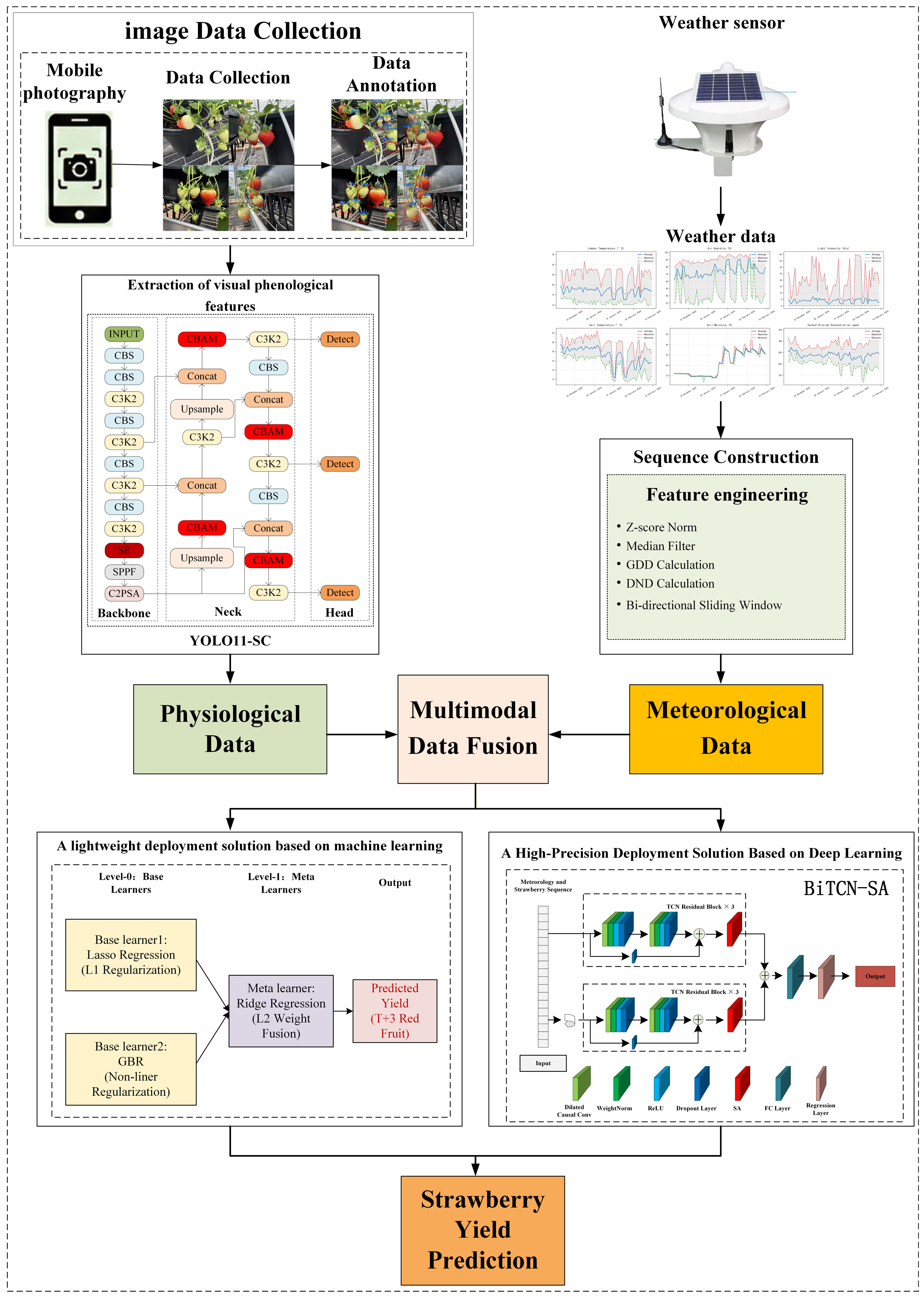
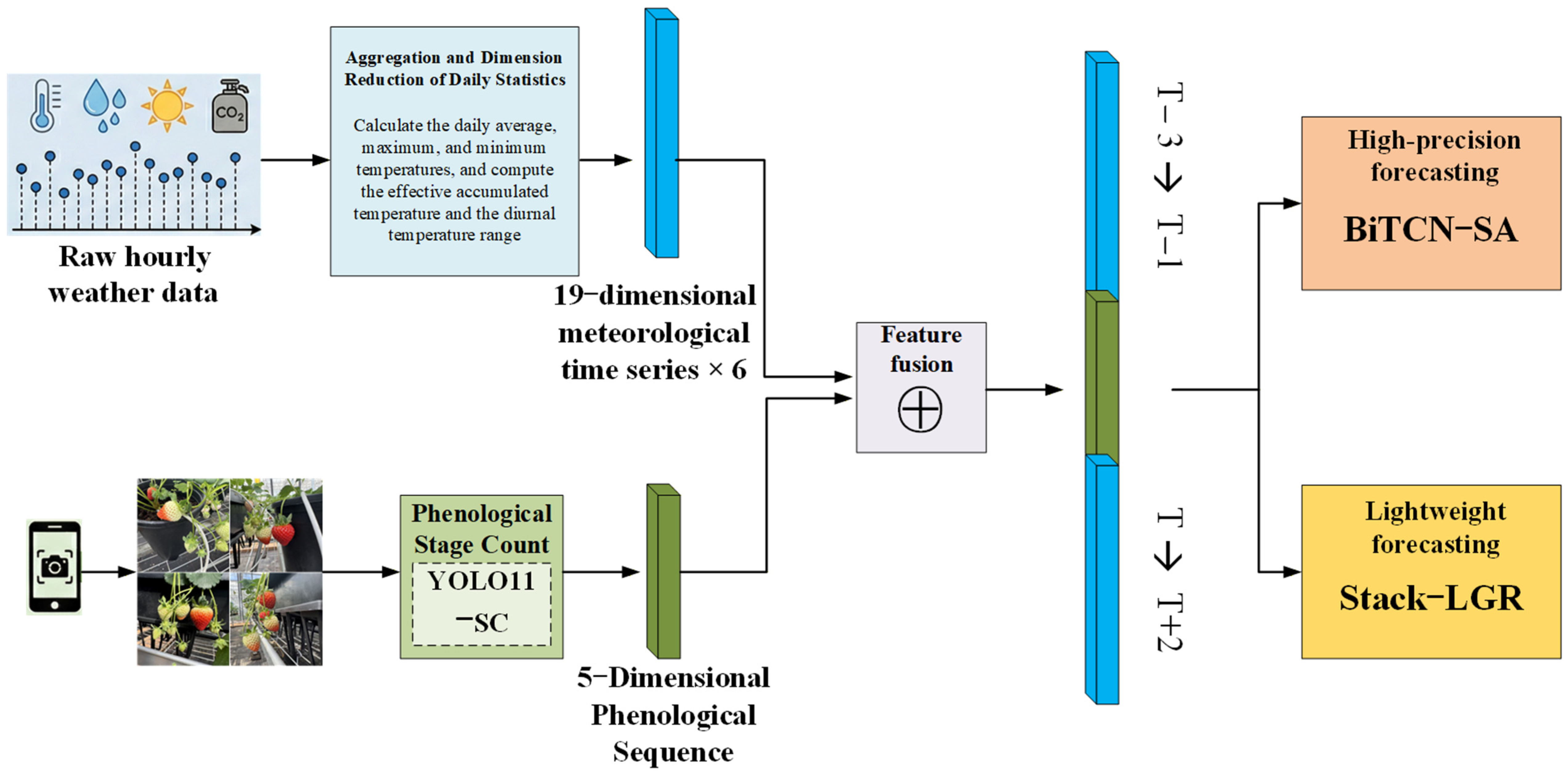
The overall architecture of the PRED-VPMS method is shown in Figure 1. The research process is primarily divided into three core stages: First, an improved object detection model is trained using image datasets collected and annotated in actual greenhouse environments, to achieve automated, high-precision extraction of physiological characteristics across multiple consecutive strawberry phenological stages. Second, microclimate meteorological sequences from the greenhouse are simultaneously acquired; through feature alignment and fusion techniques, a multi-source “meteorological–phenological” spatiotemporal sequence matrix is constructed, incorporating dynamic growth information and environmental drivers. Finally, to accommodate diverse computational requirements, this multimodal feature matrix is processed through either a deep learning model or an edge-deployed machine learning ensemble architecture, facilitating precise short-term strawberry yield prediction.

Under practical production conditions, strawberries are generally harvested at a three-day interval. Our approach adopts a three-day interval as the standard harvesting cycle. We utilize phenological information from the previous harvesting cycle, combined with meteorological sequences from both the current and preceding cycles, to predict the cumulative yield of mature fruit for the upcoming harvesting cycle.

2.1. Data Collection

The experimental data were collected from a smart agricultural glass greenhouse at Yunnan Agricultural University, Kunming, China, which features two distinct cultivation zones: potted cultivation and soilless beds mounted on lifting cultivation racks. The strawberry cultivar utilized in this study was ‘Benihoppe’. At the onset of the 72-day monitoring period, the plants were 4 months old and exhibited uniform growth. The cultivation substrate consisted of a standard commercial coconut coir mixture. Fertigation management followed a specialized nutrient solution protocol tailored for greenhouse strawberries; the electrical conductivity (EC) was strictly maintained between 0.8 and 1.2 dS/m, and the pH was adjusted to 5.8–6.2. The nutrient solution was delivered three times daily via an automated drip irrigation system (RAINGROW-M, XiaomaIOT, China). The macro-environmental control system operated under an automated ventilation schedule, which was triggered whenever ambient temperatures exceeded 28 °C.

To construct a stable image dataset for the YOLO11-SC object detector, images were actively collected from both cultivation zones. The potted strawberries were transplanted one month earlier and exhibited accelerated initial growth, facilitating early-stage phenological image acquisition. As the strawberries on the lifting racks matured, their images were subsequently captured and merged into the training repository, thereby enhancing dataset diversity across heterogeneous environmental backgrounds.

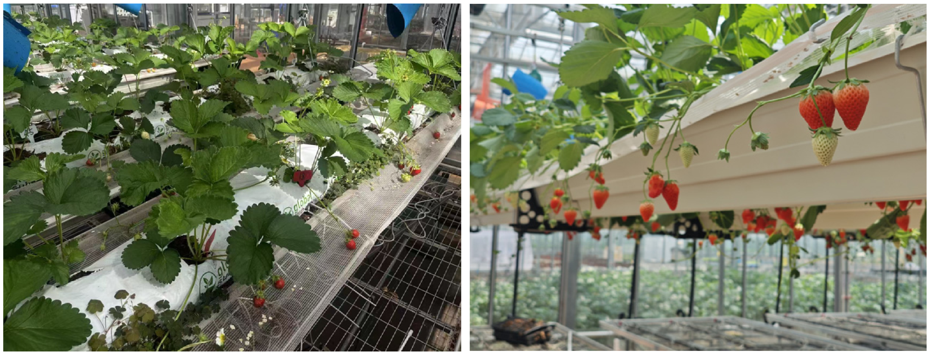
In contrast, the downstream multimodal yield prediction experiment focused exclusively on the lifting cultivation racks, as shown in Figure 2. This rack facility housed 119 soilless beds containing 595 strawberry plants, with five plants per bed. The potted cultivation zone was excluded from this yield prediction phase because it operated under a distinct fertilization management system and experienced a temporary technical issue with the soil sensor during the monitoring period. Including the potted zone would have introduced confounding environmental variables and irrecoverable data gaps. From the 595 plants on the lifting racks, 150 healthy individuals exhibiting standard growth were selected for the experimental dataset and closely monitored over the 72 days.

In this study, an individual strawberry plant was defined as the basic observational unit. The yield prediction task aimed to predict the number of red fruits produced by each strawberry plant during the next harvesting period. The complete dataset consisted of meteorological data and phenological information collected from 150 strawberry plants across 22 harvesting cycles. Each input sample corresponded to one individual strawberry plant at a specific harvesting cycle and consisted of the plant’s phenological characteristics and the corresponding 6-day meteorological data for that period. The 150 selected strawberry plants were partitioned into training and test sets at a ratio of 7:3, with 105 plants used for model training and 45 plants used for model testing. To reduce the risk of information leakage caused by spatial correlations among neighboring plants and to ensure reliable evaluation of the proposed model’s predictive performance, the 105 plants in the training set were used exclusively for model training, whereas the 45 plants in the test set were used solely for model testing.

2.1.1. Visual Phenology Data Collection and Processing

For the visual phenotyping of strawberries, on-site image acquisition was conducted in the greenhouse using a Huawei Mate 40 Pro smartphone (Huawei Technologies Co., Ltd., Shenzhen, China) with a 50-megapixel rear camera, capturing images at a standard resolution of 3840 × 2160 pixels. To ensure structural consistency and high dataset quality, a rigorous spatial protocol was maintained: the smartphone was positioned at a fixed distance of approximately 30–50 cm from the target strawberry canopy, maintaining an oblique top-down shooting angle of 45° to 60° relative to the horizontal plane of the cultivation bed to optimize the visibility of fruits.

These images were subsequently processed by the developed YOLO11-SC model for phenotypic feature extraction. The sampling period spanned from 15 December 2025, to 20 February 2026, totaling 68 days. During this period, an intermittent sampling strategy was adopted, with images of the experimental plants captured at regular three-day intervals. The core objective of this dataset is to support automated identification and quantification of various strawberry phenological stages (e.g., flower, green fruit, and pink fruit) using object detection models, thereby providing fine-grained physiological and phenotypic data for downstream yield prediction.

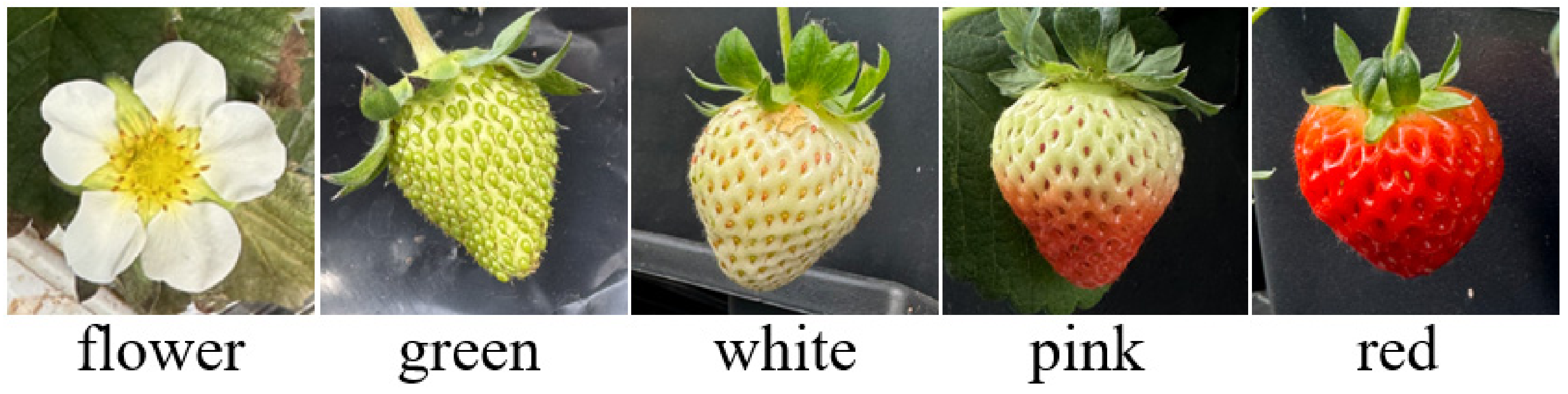
According to the developmental curve reported by Symons et al. [27], the major phenological stages of the strawberry plant exhibit significant visual differences. From flowering to maturity, strawberries primarily undergo the following stages: flower, small green, green, small white, large white, pink, and red. Because the “small green” and “green” stages exhibit high visual similarity, making accurate differentiation via computer vision challenging, these two stages were consolidated into a single “green” category. Likewise, the “small white” and “large white” stages were combined into a unified “white” category. Consequently, the final target classes for detection are defined as flower, green, white, pink, and red, as illustrated in Figure 3. The relationship between these extracted phenological features and yield prediction is detailed in

Table 1. Phenological classes used for detection and yield prediction.

Phenological Stage	Model Input Meaning	Temporal Role in Prediction
Flower	Early reproductive signal	Yield potential initialization
Green	Vegetative expansion stage	Growth accumulation phase
White	Pre-ripening transition	Sugar accumulation onset
Pink	Ripening transition state	High sensitivity to climate
Red	Harvest-ready fruit count	Final yield output

.

The image dataset was annotated using the open-source LabelMe software (version 5.1.1) to identify five strawberry phenological classes (flower, green, white, pink, and red) [28]. Each strawberry instance was manually labeled using polygon-based annotations to accurately delineate object boundaries in complex greenhouse environments. All images were annotated by a single trained annotator following a unified labeling protocol. To ensure annotation consistency, multiple rounds of internal quality checks were conducted after the initial annotation process. Specifically, randomly selected annotated images were repeatedly reviewed according to the predefined labeling criteria, and any identified inconsistencies were corrected. No independent expert validation was performed; therefore, the annotation quality control relied on the standardized annotation protocol and internal consistency assessment.

To ensure compatibility with the YOLO detection framework, a custom Python-based conversion pipeline based on Python 3.9 (Python Software Foundation, Wilmington, DE, USA) was developed to transform LabelMe JSON annotations into YOLO-format (.txt) labels. Specifically, polygonal annotations were first converted into axis-aligned bounding boxes by computing the minimum enclosing rectangle for each instance. The bounding box coordinates were then normalized with respect to image width and height and stored in the standard YOLO format as: (x_center, y_center, width, height).

This conversion procedure enables consistency between manual annotation and model training requirements while preserving spatial localization accuracy and maintaining the geometric integrity of annotated targets.

2.1.2. Collection and Processing of Meteorological Data

For meteorological data collection, a multi-parameter environmental monitoring station (ZMetpro-A, Beijing Zhiyang Technology Co., Ltd., Beijing, China) was installed in the smart agricultural glass greenhouse at Yunnan Agricultural University (102.756492° E, 25.133435° N) to systematically capture key environmental factors driving strawberry growth and development. The monitoring system integrates contact sensors deployed in the rhizosphere soil (to monitor soil temperature and moisture) and climate sensors installed on the greenhouse roof (to monitor atmospheric conditions). The system continuously monitored environmental parameters, including air temperature, soil temperature, relative humidity, soil moisture, light intensity, and CO₂ concentration. The monitoring station was calibrated according to the manufacturer’s specifications, ensuring reliable acquisition of environmental data. 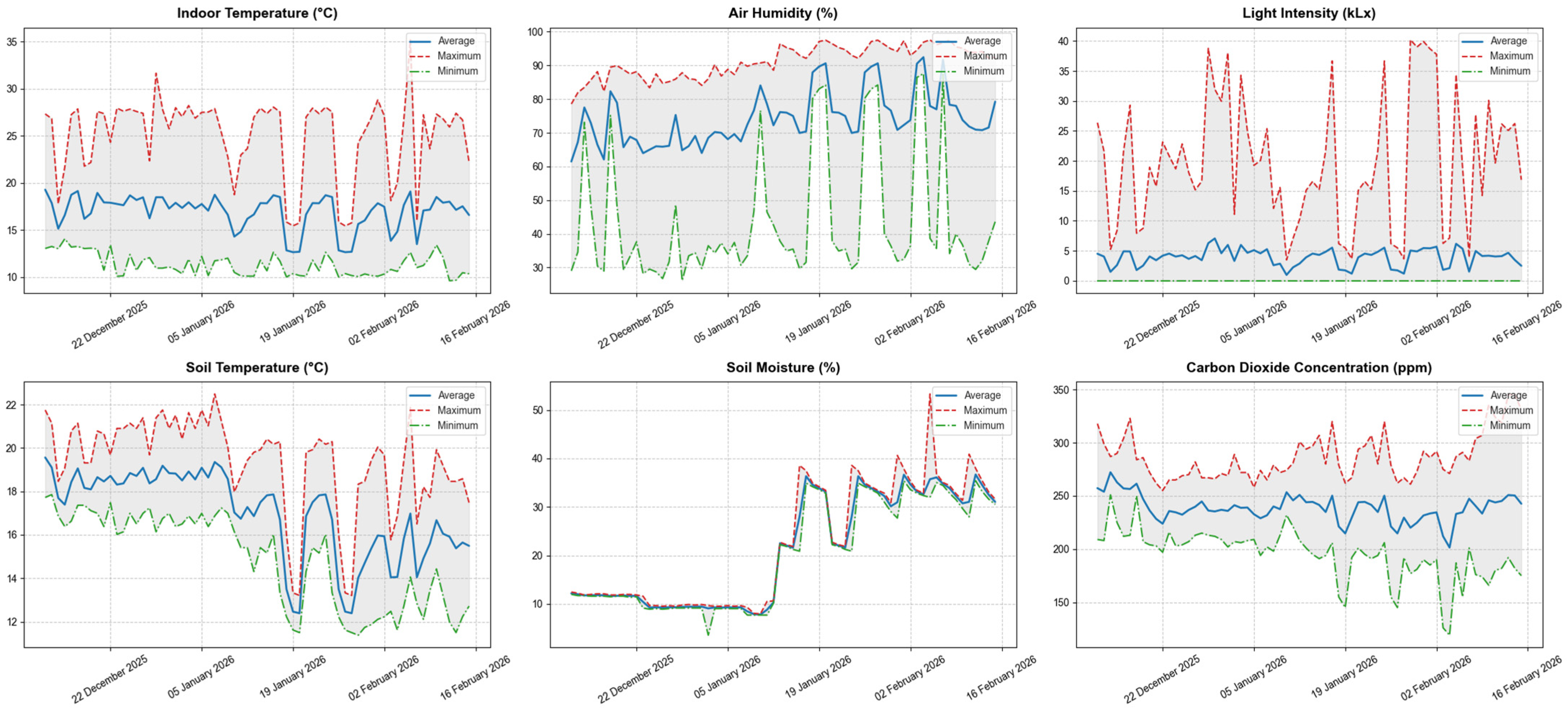The data collection frequency was set at 60-min intervals, with real-time monitoring parameters covering thermal factors (air and soil temperature), moisture factors (air humidity and soil moisture), energy factors (light intensity), and carbon source factors (CO₂ concentration). The meteorological observation period spanned from 11 December 2025 to 20 February 2026, comprising a continuous 72-day sequence, as illustrated in Figure 4.

2.2. Multi-Source Heterogeneous Data Processing and Feature Fusion

To ensure the numerical stability and phenological consistency of the input features, rigorous preprocessing and feature fusion were applied to the raw multi-source data. The specific steps are detailed as follows.

2.2.1. Meteorological Time Series Denoising and Spatio-Temporal Reconstruction

To address impulse noise and outliers caused by random environmental interference during sensor data acquisition, a sliding median filter was employed to reduce noise and smooth the data. Additionally, to address minor data gaps caused by transient communication interruptions, linear interpolation was utilized for data imputation. This process effectively eliminated abnormal fluctuations and ensured the spatiotemporal continuity of the feature matrix within subsequent sliding windows.

2.2.2. Time-Scale Alignment and Phenological Quantification

Due to the significant asymmetry in sampling frequencies between meteorological factors (60 min/reading) and visual phenological features (3 days/reading), an alignment strategy was implemented using the “day” as the base temporal unit:

• Meteorological Feature Aggregation: Meteorological data were first processed through statistical aggregation of high-frequency intraday sequences, from which daily mean, maximum, and minimum values were extracted. Based on the physiological characteristics of strawberry growth and development, biologically meaningful derived indicators, including Growing Degree Days (GDDs) and Day–Night Temperature Difference (DND), were further calculated. In this way, the raw meteorological observations were condensed into a 19-dimensional core environmental feature vector (since light intensity is zero at night, we calculated only the maximum and average light intensity values for the daily meteorological data). GDDs and DND were subsequently used as key meteorological predictors of yield.

Growing Degree Days (GDDs) were calculated using the mathematical expression shown in Equation (1).

$$GDD={\displaystyle \sum _{i=1}^n}\left({\displaystyle \frac{T_{\mathrm{m}\mathrm{a}\mathrm{x},i}+T_{\mathrm{m}\mathrm{i}\mathrm{n},i}}{2}}-T_b\right)$$

(1)

where $T_{\mathrm{m}\mathrm{a}\mathrm{x},i}$ and $T_{\mathrm{m}\mathrm{i}\mathrm{n},i}$ denote the daily maximum and minimum temperatures (°C), respectively, $T_b$ is the base temperature, and $n$ is the number of days. In this study, the base temperature for strawberries was set to 5 °C, which is widely used as the lower developmental threshold in horticultural growth modeling. The unit of GDD is °C day.

Day–Night Temperature Difference (DND) was mathematically defined asshown in Equation (2).

$$DND=T_{day}-T_{night}$$

(2)

where $T_{day}$ and $T_{night }$ represent the mean daytime and nighttime temperatures (°C), respectively.

These two indicators characterize thermal accumulation and diurnal temperature variation, both of which are critical environmental factors influencing strawberry growth, development, and fruit formation.

2.

Visual Phenological Feature Normalization: The five-dimensional phenological count vector, extracted via the developed YOLO11-SC model, was converted into a ratio vector characterizing the plant developmental status through relative abundance normalization. This step eliminated the influence of planting density variations, providing the model with phenological constraints in addition to environmental drivers.

2.2.3. Fusion Based on a “Backward–Forward” Time Window

A feature aggregation framework was constructed for $T+3$ yield prediction. The core logic of this framework lies in utilizing meteorological sequences from the 6 days preceding the prediction point to capture growth momentum, with the phenological features on day $T$ serving as the physiological anchor, as illustrated in Figure 5. The multimodal fusion occurs strictly after the object detection network and the meteorological time-series sequences are integrated only after the strawberry count features are output by the model.

• Construction of a Bidirectional Meteorological Time Series

To fully capture the microclimate dynamics affecting strawberries from fruit enlargement to color development and ripening, we extracted a 6-day meteorological time-series matrix $E\in R^{6\times 19}$ entered on the prediction base day ($T$). This matrix consists of two components: a pre-harvesting meteorological sequence ($T-3$ to $T-1$) and a post-harvesting meteorological sequence ($T$ to $T+2$). These data were obtained from sensor-based observations rather than weather forecasts. The meteorological data from the preceding three days are utilized to characterize the plant’s physiological accumulation and growth inertia during the prior stages; conversely, the meteorological data from the three days following harvesting are employed to drive the model’s estimation of the rate at which the fruit transitions to the red fruit stage. It should be noted that the meteorological data from $T$ to $T+2$ are not information available at the initial prediction time. Therefore, the current framework does not represent a fully operational forecasting system. For practical deployment, these observed meteorological data would need to be replaced with weather forecast data or prediction outputs from greenhouse climate models.

2.

Global Coupling of Heterogeneous Features

The 5-dimensional normalized phenological vector $P_T$ extracted on day $T$ is utilized as the global state feature and coupled with the 6-day meteorological sequence. Under this architecture, the 19-dimensional dynamic meteorological sequence captures the continuous evolution of environmental trends. At the same time, the 5-dimensional visual phenological information serves as a physiological background constraint, integrating with global meteorological features.

This combination yields a multimodal feature set comprising 6-day meteorological sequences and corresponding phenological information. This design achieves deep coupling between environmental drivers and actual crop load, enabling the model to effectively identify complex phenological responses characterized by differential physiological responses to identical thermal conditions, while significantly reducing data redundancy at the input layer. By integrating five-dimensional phenological information as global features with time-series meteorological observations, the model learns that, under a given current phenological state (e.g., a high proportion of pink-stage fruits), meteorological variations contribute to cumulative yield formation during the subsequent period from $T+1$ to $T+3$. This mechanism effectively alleviates the prediction lag issue commonly observed in meteorological-only models, which primarily results from their limited capability to incorporate crop physiological stages.

2.3. Methods for Extracting Visual Phenological Features

2.3.1. Base Model

In computer vision-based yield prediction systems, object detection accuracy is critical for determining the quality of the extracted phenological information for subsequent yield prediction. In this study, the YOLO11 architecture released by Ultralytics in 2024 was adopted as the base detector because it provides a favorable balance between detection accuracy, computational efficiency, and compatibility with the proposed multimodal yield prediction framework [29]. Furthermore, its lightweight design makes it well-suited for edge computing applications.

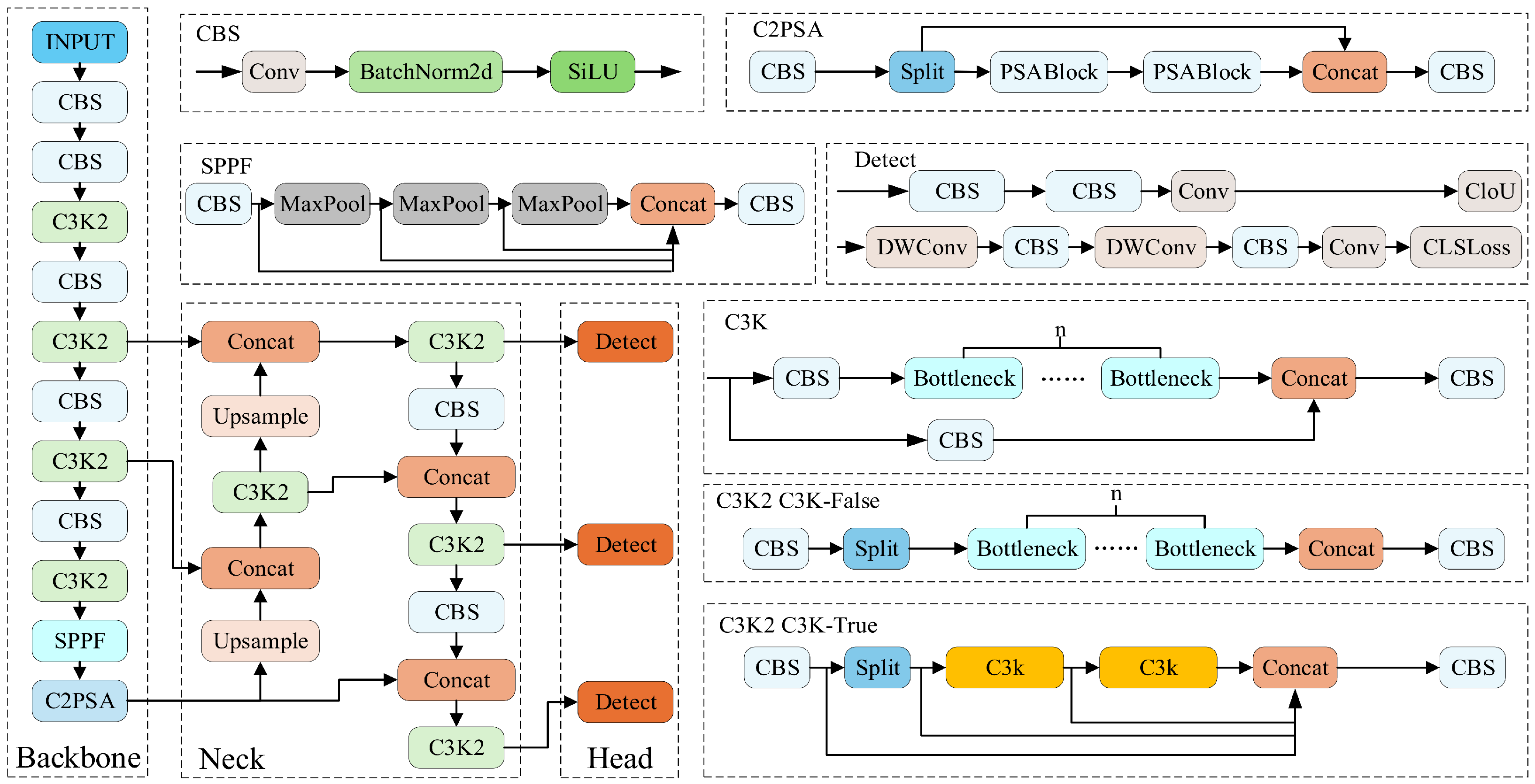
The YOLO11 series offers five scaled versions, ranging from YOLO11n to YOLO11x, to balance inference speed and computational complexity [30]. As illustrated in Figure 6, the algorithm adopts the standard “backbone–neck–head” architecture: the backbone extracts multidimensional features, the neck performs multi-scale feature fusion, and the head executes end-to-end detection. Key design components include the CBS module for enhancing feature extraction efficiency, the C3k2 module for strengthening feature representation, the SPPF module for capturing global context, and the detection head, which balances accuracy and computational overhead through lightweight depth-wise convolutions. This systematic architectural optimization improves the model’s detection performance in complex scenarios.

2.3.2. Model Improvement Strategies

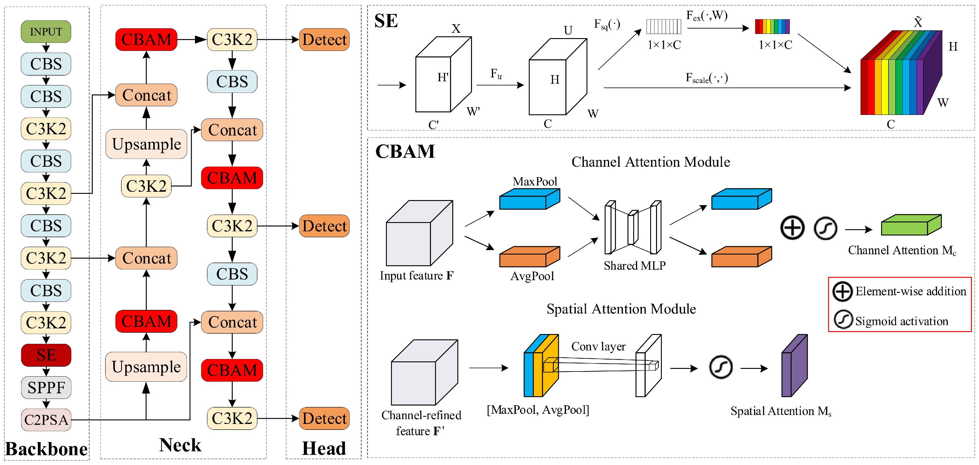
In greenhouse environments, accurately detecting strawberry targets faces two major challenges: first, fruits are frequently partially occluded by dense foliage or obstructions, leading to the loss of spatial features; second, unripe green fruits and background foliage exhibit high visual similarity. Traditional convolutional operations assign uniform weights to all channels and spatial regions during feature extraction, making it difficult for the network to prioritize salient features. To address this, we propose YOLO11-SC, a model optimized for visual phenological feature extraction tasks. This model is built on the YOLO11s baseline architecture and is illustrated in Figure 7. By strategically introducing a multi-scale attention mechanism during feature extraction and fusion, this design improves the model’s representational capabilities in complex backgrounds.

In the deep semantic representation stage of the backbone network, the Squeeze-and-Excitation (SE) attention module was integrated to dynamically recalibrate channel-wise feature responses [31]. Its mathematical formulation is expressed in Equation (3).

$$s=F_{ex}\left(z,\widehat{W}\right)=\sigma \left(g\left(z,\widehat{W}\right)\right)=\sigma \left(W_2\delta \left(W_{1}z\right)\right)$$

(3)

The SE module models channel dependencies through two core operations: Squeeze and Excitation. First, global average pooling is employed to compress the $H\times W\times C$ feature map into a $1\times 1\times C$ global descriptor, capturing the spatial distribution of the global information. Subsequently, a nonlinear mapping is constructed via two fully connected layers to generate attention weights for each channel. In the context of strawberry growth monitoring, ripe fruits (high-saturation red), canopy leaves (green), and plastic mulch (black/white) exhibit distinctly different response intensities across specific channels of the feature map. Through adaptive learning, the SE module updates the weights of channels associated with fruit phenotypic features (e.g., specific chromatic characteristics and spherical textures) while actively suppressing irrelevant background channels. This recalibration step ensures that the feature streams entering the SPPF spatial pyramid pooling layer possess high discriminative power, laying a stable foundation for subsequent high-level semantic extraction.

The Neck network serves as a central hub for multi-scale feature transmission and aggregation; however, its core challenge lies in the accumulation of noise induced by feature concatenation operations. To further improve representational precision during the feature fusion stage, we introduced the Convolutional Block Attention Module (CBAM) immediately following all concatenation operations [32]. This module adaptively refines the intermediate feature maps by sequentially deriving attention maps along both the channel and spatial dimensions. Specifically, assuming the input intermediate feature map is denoted as $F\in R^{C\times H\times W}$, the sequential processing steps of the CBAM are defined by Equations (4) and (5).

$$F^{\prime }=M_c\left(F\right)\otimes F$$

(4)

$$F^{″}=M_s\left(F^{\prime }\right)\otimes F^{\prime }$$

(5)

where $M_c\in R^{C\times 1\times 1}$ denotes the channel attention mapping vector, $M_s\in R^{1\times H\times W}$ denotes the spatial attention mapping matrix, and ⊗ denotes element-wise multiplication. In the above operations, the intermediate feature F first undergoes important feature filtering via the channel attention submodule (CAM) to generate a weighted feature map $F^{\prime }$; subsequently, $F^{\prime }$ is fed into the spatial attention submodule (SAM) for saliency region localization, ultimately outputting a refined feature representation $F^{″}$.

This sequential cascade architecture demonstrates significant advantages in the strawberry detection task: the channel-wise weight distribution derived from $M_c$ helps the model identify the phenotypic channels most discriminative for yield prediction after feature concatenation. Meanwhile, the introduction of $M_s$ enables the model to continue assigning higher activation weights to the key geometric pixels in exposed fruit regions, even under severe mutual occlusion, thereby producing stable local spatial features.

This ability to capture spatially salient regions guides the model to effectively bypass occluding elements (e.g., leaf margins and trellis wires). By precisely focusing its activation weights on exposed fruit areas, the network significantly reduces the false negative rate in densely clustered scenes.

2.4. Methods for Short-Term Strawberry Yield Prediction

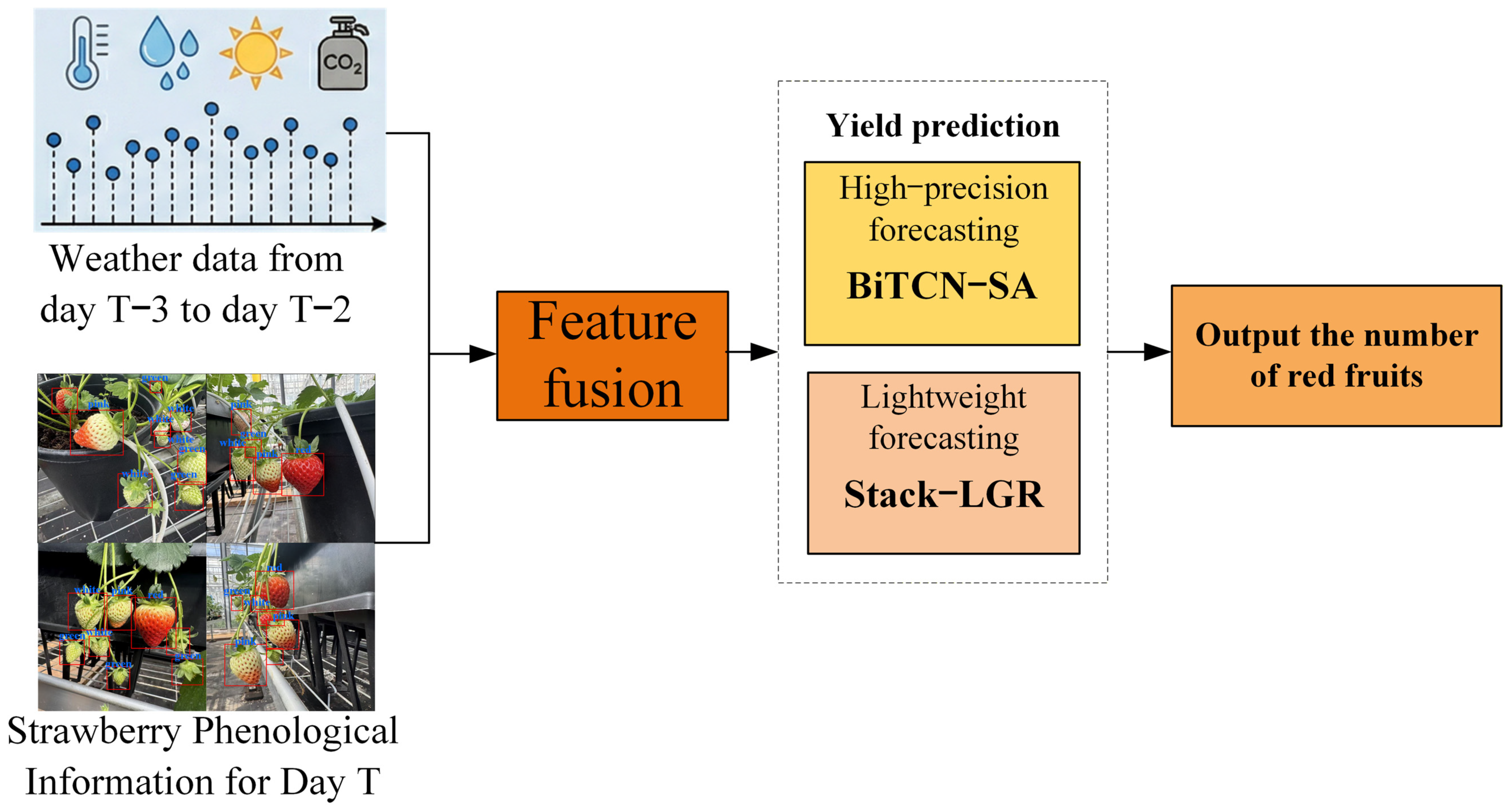
As depicted in Figure 8, the PRED-VPMS method performs short-term yield estimation by constructing a multi-source spatiotemporal feature matrix. This framework uses the meteorological data from the three days prior to harvesting and visual phenological information from multiple developmental stages of strawberries as a baseline, and deeply integrates meteorological data for the three days following harvesting (including the harvesting day) to achieve accurate predictions of the yield (the number of red fruits) of mature fruit over the next three days. Specifically, an object detection model is first employed to extract phenological statistics of strawberry plants, while environmental sensors deployed within the greenhouse continuously collect meteorological data. These phenological and meteorological data are then fused and input into the yield prediction model, which ultimately outputs the predicted number of red fruits. In this study, the training and evaluation of the yield prediction model were conducted using fruit counts generated by the YOLO-based detection model rather than manually annotated values; therefore, detection errors are propagated into the yield prediction model during both the training and testing stages.

2.4.1. A Lightweight Machine Learning-Based Yield Prediction Method

We propose a lightweight, short-term yield prediction framework that integrates computer vision-based phenotypic sensing with a bidirectional, time-series, environment-driven approach. This framework first enhances feature quality through rigorous data preprocessing protocols, and subsequently utilizes Stack-LGR to simultaneously account for growth inertia and meteorological data from the next harvesting period. This approach thereby achieves accurate predictions of red fruit yield on day $T+3$. 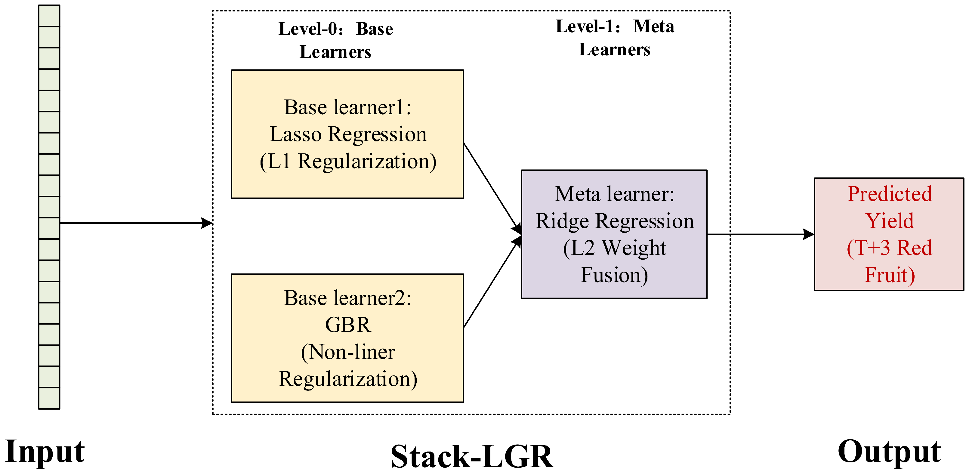As illustrated in Figure 9, the model architecture consists of two primary components: Level-0 base learners, responsible for the parallel extraction of heterogeneous feature representations, and a Level-1 meta-learner, which executes global weight optimization and nonlinear fusion.

The Stack-LGR model adopts a stacked ensemble architecture and employs a two-layer learning mechanism to deeply explore the nonlinear mapping relationships among heterogeneous multi-source information. Its mathematical formulation is given by Equation (6).

$$Y_{T+1\to T+3}=M_{meta}\left[\sum _{i=1}^n{B}_i\left(P_T,W_{T-3\to T-1},F_{T\to T+2}\right)\right]$$

(6)

Here, the output $Y_{T+1\to T+3}$ represents the cumulative yield of mature fruit over the current harvesting period (days $T+1$ to $T+3$). The input feature set consists of three components: $P_T$ denotes the five-stage phenological index values for strawberries extracted in real-time by the YOLO11-SC model on day $T$, forming the static physiological baseline for yield prediction; $W_{T-3\to T-1}$ represents the meteorological time series for the past three days (excluding the reference day), serving as the growth inertia that characterizes the recent accumulation of photosynthetic products in the crop; $F_{T\to T+2}$ represents the sensor-observed meteorological sequence collected over the period from day $T$ to $T+2$, which is incorporated as a dynamic environmental driver regulating fruit coloration and maturation. Importantly, all meteorological inputs are derived from in situ observations rather than forecasted data. $B_i$ and $M_{meta}$ represent the primary learners based on Lasso and gradient boosting regression (GBR), respectively, as well as the meta-learner based on ridge regression.

In the primary learning stage ($B_i$), we constructed a feature extraction mechanism driven by a heterogeneous algorithm in parallel. This mechanism achieves trend-fluctuation feature decoupling by integrating Lasso regression with GBR: on the one hand, it utilizes the L1 regularization property of Lasso regression to efficiently screen key factors from high-dimensional data, thereby stablely characterizing the linear baseline trend followed by crop growth development; on the other hand, it leverages the strengths of GBR in residual learning and nonlinear space exploration to capture complex nonlinear disturbances caused by sudden changes in greenhouse meteorological factors (such as abrupt changes in light intensity or CO₂ fluctuations). This complementary architecture of linear and nonlinear components lays a high-dimensional, phenologically interpretable feature foundation for subsequent global optimization of the meta-learner.

In the meta-learning stage ($M_{meta}$), we introduce ridge regression with L₂ regularization constraints to construct a secondary fusion architecture. Its core mechanism lies in mapping the prediction outputs of primary heterogeneous learners to a meta-feature space and dynamically optimizing weight allocations via regularization penalties to effectively suppress the model’s excessive sensitivity to specific meteorological disturbances or local data noise. This strategic weighted fusion mechanism not only mitigates the risk of overfitting in ensemble systems but also enables the model to achieve significantly superior generalization and predictive stability compared to individual base learners in complex, variable greenhouse environments.

2.4.2. A High-Precision Deep Learning-Based Yield Prediction Method

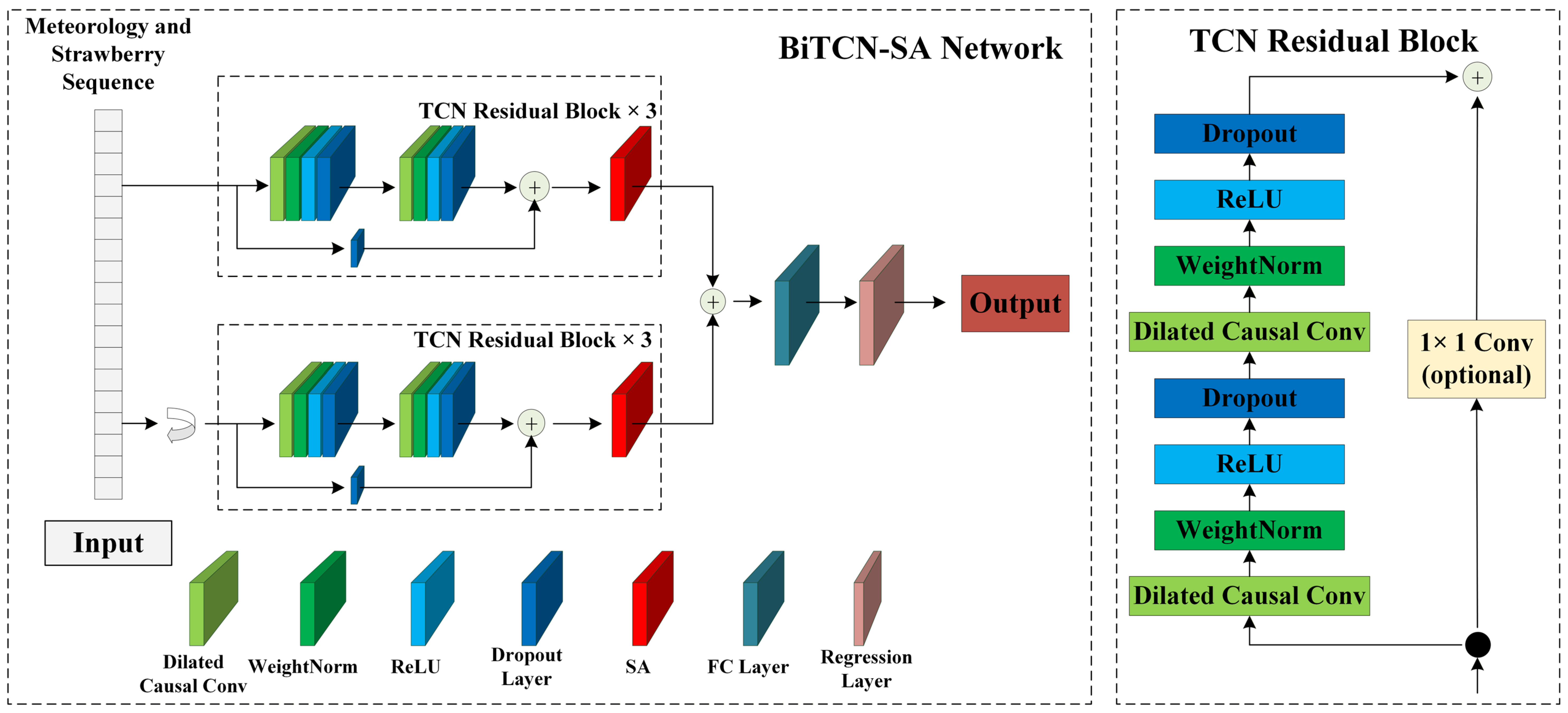
The meteorological and strawberry phenological data utilized in this study exhibit pronounced nonlinear time-series characteristics. To address the inherent time-lag and complexity of meteorological influences on strawberry growth, as well as the generalization challenges under specific greenhouse conditions, we propose a prediction architecture: the Bidirectional Temporal Convolutional Network with Self-Attention (BiTCN-SA). By embedding self-attention mechanisms into both the forward and reverse branches of the BiTCN, this architecture effectively captures long-range bidirectional temporal dependencies within sequences and improves global feature extraction. As illustrated in Figure 10, the model architecture comprises a sequence input layer, a core BiTCN-SA feature extraction module, a fully connected layer, and an output layer.

To capture bidirectional temporal dependencies in meteorological and phenological sequences, a Bidirectional Temporal Convolutional Network (BiTCN) is adopted. The model consists of two parallel temporal convolutional streams, namely a forward TCN branch and a backward TCN branch, which process the input sequence in the chronological and reverse temporal directions, respectively. Each branch is composed of N = 3 stacked residual TCN blocks. Within each block, causal 1D convolutions with kernel size k = 3 are employed, and dilation factors follow an exponential schedule d = {1, 2, 4} to enlarge the temporal receptive field. Residual connections are introduced to stabilize gradient propagation and improve feature reuse. To enhance feature representation, a spatial attention (SA) mechanism is inserted after each TCN residual block in both forward and backward branches. The SA module adaptively recalibrates feature responses by emphasizing informative temporal features and suppressing irrelevant noise in both spatial and channel dimensions. The outputs of the forward and backward branches are concatenated along the feature dimension to form a unified bidirectional representation. Finally, the fused features are passed through a fully connected regression layer to generate the final yield prediction.

Bidirectional Temporal Convolutional Network Module

Temporal convolutional networks (TCNs), introduced by Bai et al. [33], represent a significant architectural advancement over traditional Convolutional Neural Networks (CNNs) for sequence modeling, and have been widely adopted for time-series prediction in fields such as finance, power systems, and meteorology. TCNs utilize causal convolutions to strictly prevent future information leakage, dilated convolutions to exponentially expand the receptive field, and residual connections to mitigate gradient vanishing and overfitting issues. Furthermore, they support highly parallelized computation, efficient training, and stable modeling of long-term dependencies. For a data sequence $\left[X_0,X_1,\dots ,X_{t-1},X_t\right]$, after applying causal convolution, the output $y_t$ at time step $t$ depends exclusively on the input values at time step $t$ and prior time steps from the preceding layer. This mathematical relationship is defined in Equation (7).

$$y_t=f\left(X_0,X_1,\dots X_{t-1},X_t\right)$$

(7)

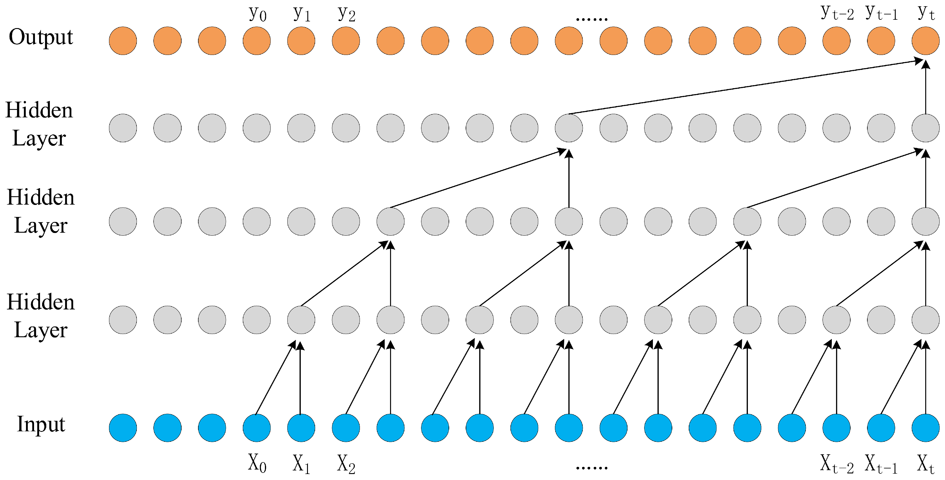
In the feature extraction stage, we employ Bidirectional Temporal Convolution (BiTCN) to process the input meteorological spatiotemporal sequence $X\in R^{T\times C}$. To effectively capture long-range temporal dependencies in meteorological sequences with fewer network layers, the BiTCN residual blocks incorporate dilated convolutional operators. As shown in Figure 11, dilated convolution expands the receptive field by inserting “holes” between the elements of the convolution kernel, thereby providing stronger feature representation capabilities compared to standard convolution without increasing the number of parameters or computational complexity. When processing a one-dimensional meteorological data sequence $\left[x_0,x_1,\dots ,x_{t-1}{,x}_t\right]$, the output value $h\left(t\right)$ of the hidden layer at time t is given by Equation (8).

$$h\left(t\right)=\left(x\ast df\right)\left(t\right)={\displaystyle \sum _{i=0}^{k-1}}f\left(i\right)·X_{t-d·i}$$

(8)

where $h\left(t\right)$ is the hidden layer output of the dilated convolution at time t, $f\left(i\right)$ represents the i-th element of the convolution kernel, $k$ is the kernel size, $d$ is the dilation factor, and $X_{t-d·i}$ is the corresponding sequence element after interval sampling. By doubling $d$ layer by layer, the model can effectively cover a 6-day observation period and capture global environmental features.

Furthermore, to enhance the model’s ability to predict meteorological trends, it employs a bidirectional architecture to perform temporal convolutions in parallel. It fuses the forward and backward features via concatenation (⊕). Its mathematical formula is shown in Equation (9).

$$H_{TCN}=\underset{h}{\to }\oplus \underset{h}{\leftarrow }$$

(9)

This design enables the generated feature map $H_{TCN}$ to simultaneously incorporate bidirectional dependencies—both past and future (relative to the current sequence point)—providing a stable feature foundation for yield prediction.

Self-Attention Mechanism Module

The self-attention mechanism simulates the brain’s process of selectively focusing on important information from a large volume of data. To address the issue of uneven contributions to yield by meteorological factors across different growth stages, we introduced the self-attention mechanism after BiTCN. This mechanism maps the feature map $H_{TCN}$ to a query matrix ($Q$), a key matrix ($K$), and a value matrix ($V$). Calculating the correlation weights within the time series enhances the importance of key information. Its mathematical formulation is given by Equation (10).

$$Attention\left(Q,K,V\right)=softmax\left({\displaystyle \frac{Q{K}^T}{\sqrt{d_k}}}\right)V$$

(10)

Here, $\sqrt{d_k}$ serves as a scaling factor to maintain gradient stability. In predictive practice, the SA module can automatically identify extreme temperature differences or changes in light intensity—such as those occurring 1–2 days before the prediction date—and assign them higher weights, thereby enhancing the model’s sensitivity to sudden environmental fluctuations.

3. Results

3.1. Visual Phenological Feature Extraction Model

3.1.1. Training Environment and Evaluation Metrics

To quantitatively assess the detection performance of the YOLO11-SC model, precision ($P$), recall ($R$), mean average precision ($mAP$), and F1-score (F1) were adopted as evaluation metrics. Their respective calculation formulas are defined in Equations (11)–(14).

$$P={\displaystyle \frac{TP}{TP+FP}}$$

(11)

$$R={\displaystyle \frac{TP}{TP+FN}}$$

(12)

$$mAP={\displaystyle \frac{{\displaystyle {\sum }_1^N}{\int }_0^{1}P\left(R\right)dR}{N}}$$

(13)

$$F1={\displaystyle \frac{2PR}{P+R}}$$

(14)

where $TP$ (True Positives) represents the number of correctly identified strawberry fruits, $FP$ (False Positives) is the number of incorrectly identified background instances as fruits, and $FN$ (False Negatives) denotes the number of missed strawberry targets. $N$ indicates the total number of test sample categories, which is set to $N=5$. Furthermore, $mAP@0.5$ denotes the $mAP$ value evaluated at an Intersection over Union (IoU) threshold of 0.5, whereas $mAP@[0.5:0.95]$ represents the average $mAP$ calculated across various IoU thresholds (ranging from 0.5 to 0.95 in increments of 0.05).

3.1.2. Analysis of Model Testing Results

The dataset utilized for strawberry phenological stage detection comprised 784 original images, with each image containing between 1 and 8 detectable strawberry instances across five phenological categories (flower, green, white, pink, and red). To ensure balanced representation of all categories, the distribution of annotated instances before and after data augmentation is summarized in

Table 2. Distribution of strawberry phenological classes before and after data augmentation.

Phenological Class	Original Dataset	Augmented Dataset
Flower	394	1598
Green	1121	4458
White	806	3160
Pink	592	2368
Red	762	3050

. All samples in the dataset were annotated by a single trained annotator following a unified labeling protocol to ensure consistency across phenological categories.

To mitigate overfitting and improve model generalization, data augmentation was applied exclusively to the training set, including geometric transformations and photometric variations. After augmentation, the number of annotated instances increased significantly, resulting in a more balanced class distribution, as shown in Table 2. Specifically, the augmented dataset contains 1598 flower instances, 4458 green instances, 3160 white instances, 2368 pink instances, and 3050 red instances.

The dataset was split into training and test sets at an 8:2 ratio, yielding 3135 training images and 157 test images. This stratified construction ensures that all phenological stages are adequately represented in both the training and evaluation phases, thereby improving the stability of the proposed YOLO11-SC model under complex greenhouse conditions.

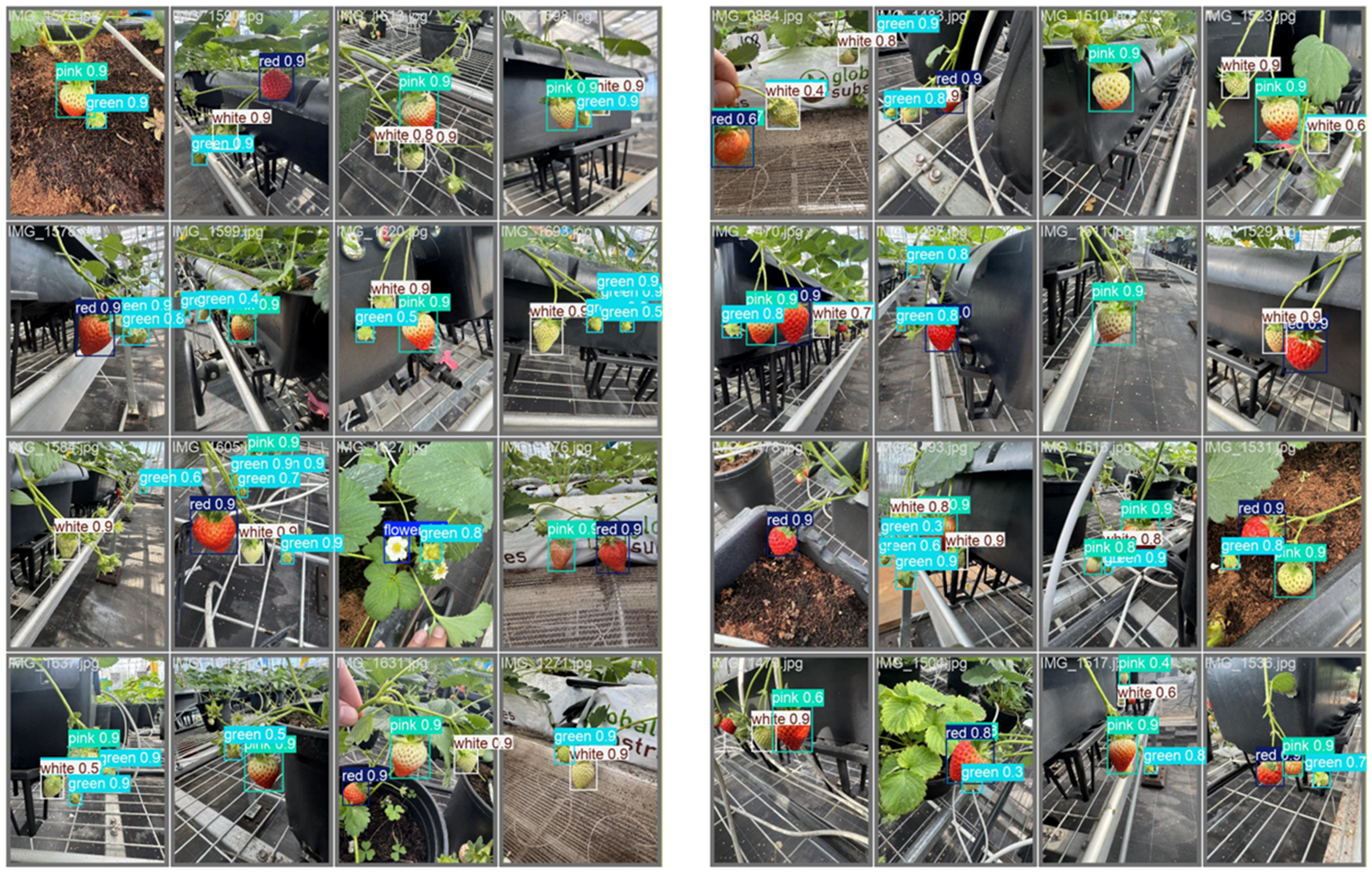
As illustrated in Figure 12, the system effectively recognized the diverse phenological stages. Flowers exhibited the highest detection confidence (ranging from 0.9 to 1.0) owing to their highly distinct morphological divergence from other targets. Green fruits were consistently detected with confidence scores ranging from 0.3 to 0.9. Because the phenotypic transition from green to white fruit involves subtle visual differentiation, the confidence lower bound for white fruits was correspondingly lower (0.4 to 0.9). Conversely, pink and red fruits exhibit highly distinctive chromatic signatures, facilitating clear separation from the other categories. Their confidence levels ranged from 0.4 to 0.9 and from 0.6 to 1.0, respectively, providing a highly reliable basis for visual tracking of the periodic volatility inherent in actual red fruit production cycles.

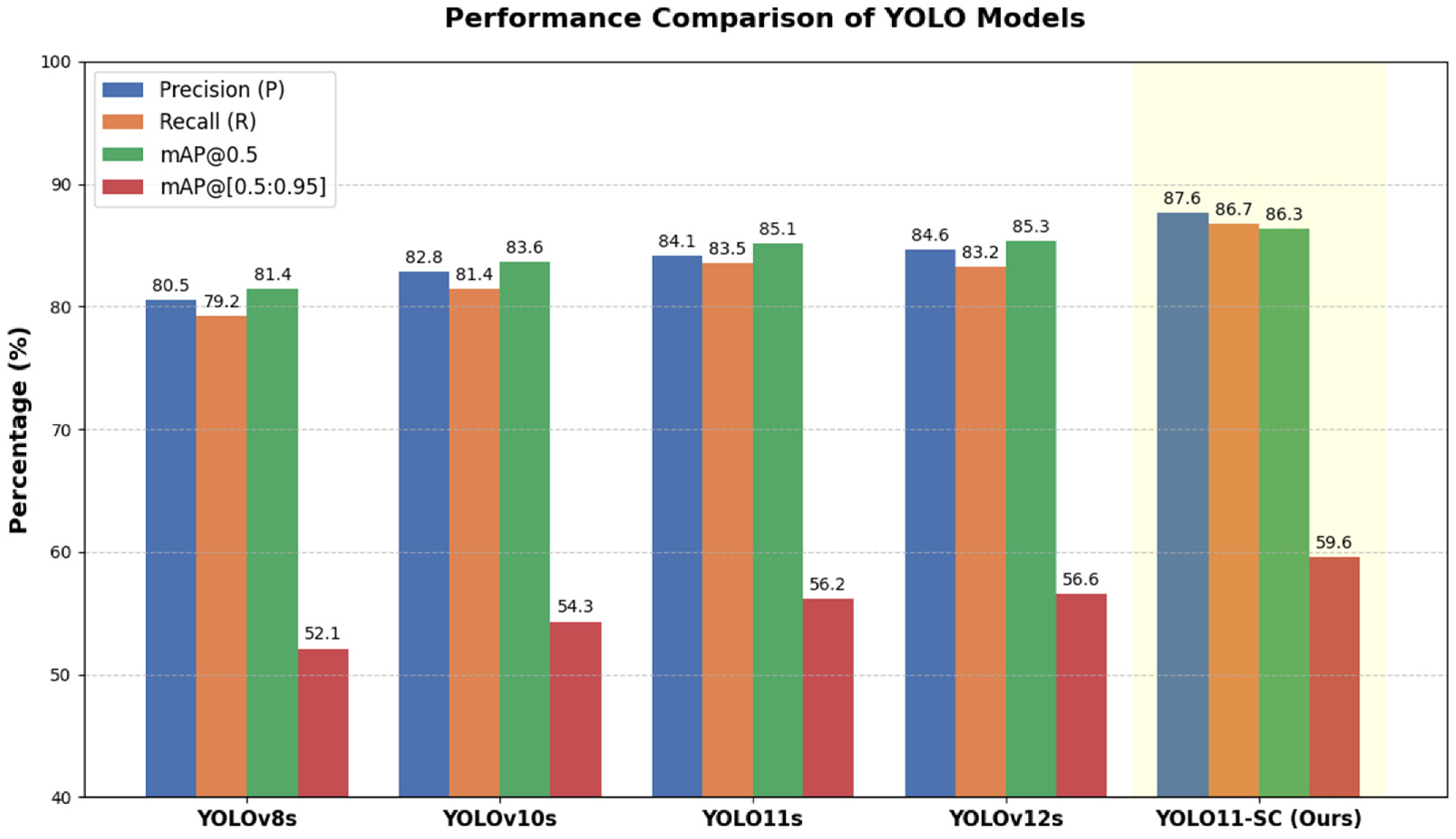
The proposed YOLO11-SC, along with the baseline YOLOv8, YOLOv10, YOLOv11, and YOLOv12 models, was trained on the augmented training set and subsequently evaluated on the independent test set. The evaluation metrics, including precision ($P$), recall ($R$), $mAP@0.5$, and $mAP@[0.5:0.95]$, were calculated for each of the five architectures. To ensure a fair comparison and mitigate the confounding effects of varying network capacities, the small (‘s’) scaling variants were uniformly selected for both the proposed model and all baseline configurations, thereby comprehensively balancing detection accuracy and model size. The comparative test results are comprehensively summarized in

Table 3. Quantitative comparison of the detection performance of different models.

Model	P/%	R/%	F1/%	mAP@0.5/%	mAP@[0.5:0.95]/%
YOLOv8s	80.5	79.2	79.8	81.4	52.1
YOLOv10s	82.8	81.4	82.1	83.6	54.3
YOLO11s	84.1	83.5	83.8	85.1	56.2
YOLOv12s	84.6	83.2	83.9	85.3	56.6
YOLO11-SC	87.6	86.7	87.1	86.3	59.6

and illustrated in Figure 13.

An analysis of the experimental metrics reveals that the proposed YOLO11-SC model achieves a Precision ($P$) of 87.6%, a Recall ($R$) of 86.7%, an $mAP@0.5$ of 86.3%, and an $mAP@[0.5:0.95]$ of 59.6%. Compared with baseline models, YOLO11-SC demonstrates consistent improvements across most evaluation metrics, suggesting better detection and localization performance in complex greenhouse environments.

3.1.3. Ablation Studies

To evaluate the individual and synergistic contributions of the SE and CBAMs within the proposed YOLO11-SC architecture, ablation studies were conducted on the test set. We systematically compared the baseline YOLO11s, the YOLO11s integrated exclusively with the SE module (Model 1), the YOLO11s integrated exclusively with the CBAM (Model 2), and the final YOLO11-SC model. The quantitative results of these experiments are summarized in

Table 4. Comparison of ablation experiment results.

Model	SE Module	CBAM	P/%	R/%	mAP@0.5/%	Params/M	GFLOPs	FPS/ms
YOLO11s	×	×	84.1 ± 0.18	83.5 ± 0.21	85.1 ± 0.16	9.5	22.1	9.87
Model 1	√	×	84.7 ± 0.15	84.2 ± 0.19	84.4 ± 0.20	13.7	43.0	9.37
Model 2	×	√	85.3 ± 0.17	84.5 ± 0.16	85.7 ± 0.14	13.8	42.1	9.20
YOLO11-SC	√	√	87.6 ± 0.12	86.7 ± 0.15	86.3 ± 0.13	14.2	45.6	9.05

, where “√” indicates that the corresponding module was included, whereas “×” indicates that it was not included. The ablation experiments were repeated three times using different random seeds, and the results are reported as mean ± standard deviation to evaluate model stability and reduce the influence of random initialization.

The ablation study results and computational efficiency analysis jointly provide a comprehensive evaluation of the proposed YOLO11-SC framework. As shown in the experimental results, compared with the baseline YOLO11s model, incorporating only the SE module (Model 1) leads to a slight decrease in mAP@0.5, despite marginal improvements in precision and recall. This suggests that although SE enhances channel-wise feature recalibration, it may suppress fine-grained spatial information that is critical for detecting small, densely distributed fruits under occlusion and complex lighting conditions. In contrast, the CBAM-only model (Model 2) consistently improves all evaluation metrics, indicating that the additional spatial attention mechanism effectively strengthens feature representation by jointly modeling channel and spatial dependencies.

Notably, the proposed YOLO11-SC model, which integrates both SE and CBAM attention mechanisms, achieves the best overall performance among all variants, reaching an mAP@0.5 of 86.3% (mean value). This improvement indicates that the two attention mechanisms provide complementary feature enhancement rather than redundant information. Specifically, SE enhances channel-wise feature recalibration by emphasizing more informative feature responses, whereas CBAM further incorporates spatial attention to improve the localization of discriminative regions. The combination of channel and spatial feature refinement enables YOLO11-SC to achieve more accurate strawberry phenological detection.

In terms of computational efficiency, the baseline YOLO11s model contains 9.5M parameters and 22.1 GFLOPs, with an inference time of 9.87 ms per image. After introducing the SE module (Model 1), the model complexity increases to 13.7M parameters and 43.0 GFLOPs, accompanied by a slight reduction in inference time to 9.37 ms per image. Similarly, the CBAM-enhanced model (Model 2) contains 13.8M parameters and 42.1 GFLOPs, with an inference time of 9.20 ms per image. These results indicate that incorporating attention mechanisms inevitably introduces additional computational overhead due to the increased feature refinement operations.

The proposed YOLO11-SC model further integrates SE and CBAMs into different feature extraction stages, resulting in 14.2M parameters and 45.6 GFLOPs, with an inference time of 9.05 ms per image. Although the hybrid attention architecture introduces slightly higher computational complexity compared with the single-attention variants, this additional cost is accompanied by the highest detection performance. The marginal increase in inference latency demonstrates that YOLO11-SC effectively balances enhanced feature representation capability and computational efficiency while maintaining near real-time inference capability.

Overall, YOLO11-SC achieves a favorable trade-off between detection accuracy and model complexity. By jointly exploiting channel-wise feature recalibration and spatial attention enhancement, the proposed framework improves strawberry phenological detection performance without causing substantial degradation in inference efficiency, making it suitable for practical strawberry phenological monitoring applications.

3.1.4. Visual Analysis of Attention Mechanisms

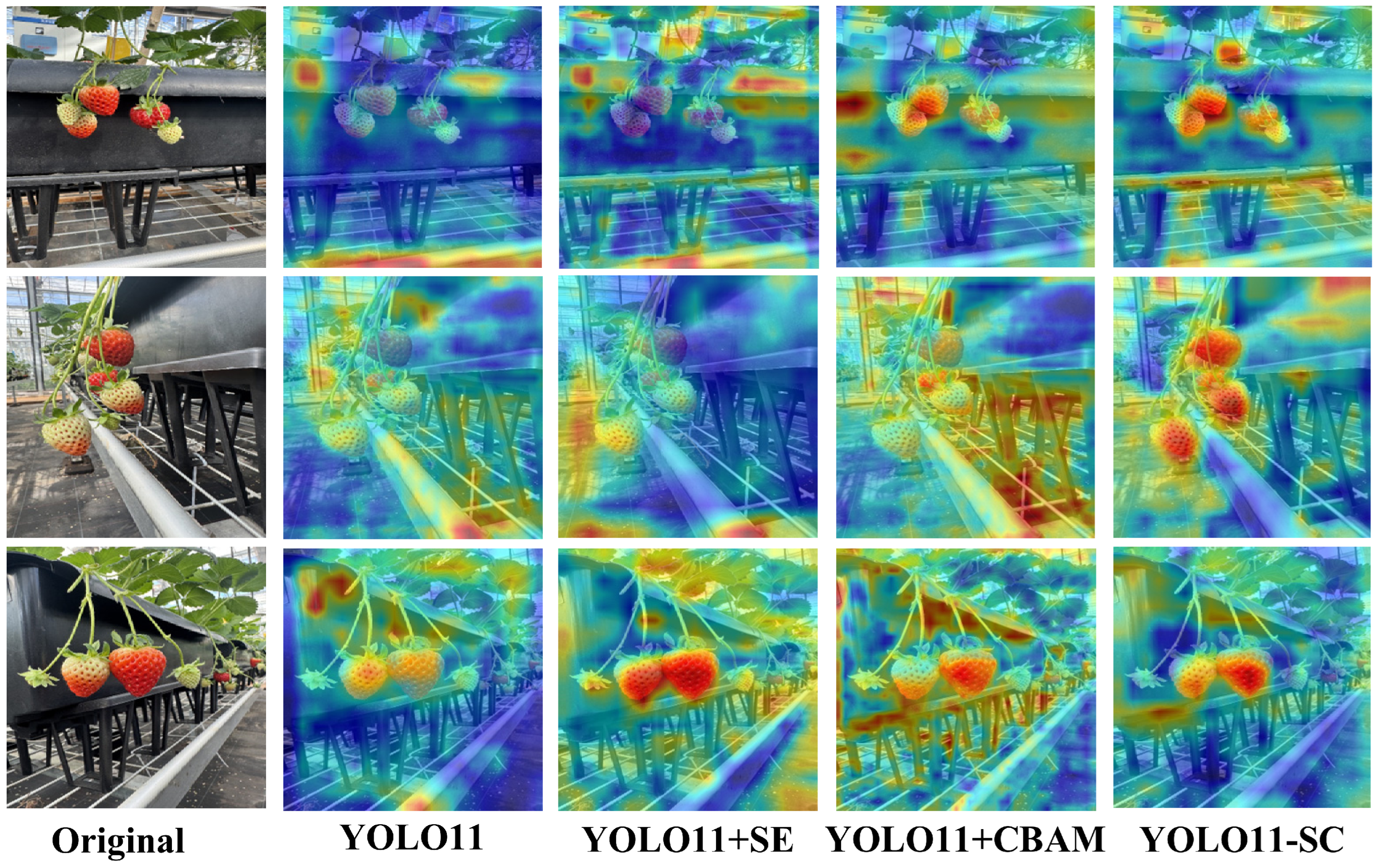
To further elucidate the underlying mechanisms by which the different attention modules modulate feature extraction in greenhouse strawberries, Gradient-weighted Class Activation Mapping (Grad-CAM) was employed [34]. As illustrated in Figure 14, this technique visualizes and compares the spatial activation heatmaps across the various stages of the ablation experiments. In these heatmaps, warmer colors (e.g., red) indicate regions where the network assigns the highest activation weights and focuses its attention. Conversely, cooler colors (e.g., blue) denote areas of diminished attention or active background suppression.

Specifically, Grad-CAM was applied to the final convolutional feature layer of the detection head in the YOLO11-SC model, as this layer preserves high-level semantic information while maintaining spatial localization capability. For visualization analysis, three representative images exhibiting fruit occlusion and diverse phenological stages were selected from the test set.

The comparative visualization in Figure 14 shows a progressive improvement in the network’s feature-focusing capabilities. Initially, when confronted with complex controlled-environment agriculture settings, the feature activation regions of the baseline YOLO11s architecture exhibit pronounced spatial dispersion and boundary spillover. Specifically, in areas obscured by foliage or characterized by cluttered backgrounds, the baseline model erroneously assigns excessive activation weights to non-informative regions, leading to insufficient focus on the actual strawberry targets.

Following the integration of standalone attention mechanisms, the network’s perceptual capabilities were enhanced across distinct dimensions. Benefiting from channel-wise weight recalibration via the Squeeze-and-Excitation module, the YOLO11s+SE variant (Model 1) demonstrated significantly improved sensitivity to strawberry-specific features (such as chromatic signatures and surface textures). This was evidenced by a marked increase in peak activation intensities within the heatmaps; however, its spatial boundaries remained relatively diffuse. In contrast, by introducing a spatial attention sub-module, the YOLO11s+CBAM variant (Model 2) exhibited superior boundary delineation in scenarios involving densely overlapping fruits, effectively decoupling the features of adjacent targets. Nevertheless, it still demonstrated limitations in capturing global semantic context under conditions of severe occlusion.

Ultimately, through the synergistic integration of the dual attention mechanisms, the proposed YOLO11-SC architecture demonstrated the most refined and stable feature representation capabilities. As evidenced in the rightmost column of the heatmaps, regardless of challenging scenarios involving dense fruit overlapping, severe canopy occlusion, or extreme non-uniform illumination, the peak activation regions of the YOLO11-SC converge precisely and compactly onto the exposed geometries of the strawberry targets. Concurrently, complex background environmental noise is maximally suppressed, resulting in distinctly cooler spectral tones.

These visualization results mechanistically validate the quantitative accuracy improvements detailed in Table 4 by elucidating the underlying nature of the deep learning feature responses. Specifically, the synergistic interaction between the SE and CBAMs successfully mitigates the inherent limitations of standard convolutional operations. This highly focused visual perception capability enables the network to accurately and automatically extract the multi-stage phenological evolutionary traits of the strawberries. Consequently, it establishes a highly reliable data foundation for the downstream construction of high-dimensional spatiotemporal feature matrices and, ultimately, precise short-term yield prediction.

3.2. A Lightweight Machine Learning-Based Yield Prediction Method

3.2.1. Performance Evaluation and Comparison of the Stack-LGR Model

All machine learning experiments were implemented in Python using scikit-learn (version 1.3.0). To ensure reproducibility and prevent feature scale bias, all input variables were normalized using StandardScaler before model training.

The base learners include Lasso regression, gradient boosting regression (GBR), and ridge regression. The hyperparameters are defined as follows: Lasso (alpha = 0.001), ridge (alpha = 1.0), and GBR (n_estimators = 100, learning_rate = 0.05, max_depth = 5, subsample = 0.8). The meta-learner adopts ridge regression for final prediction fusion.

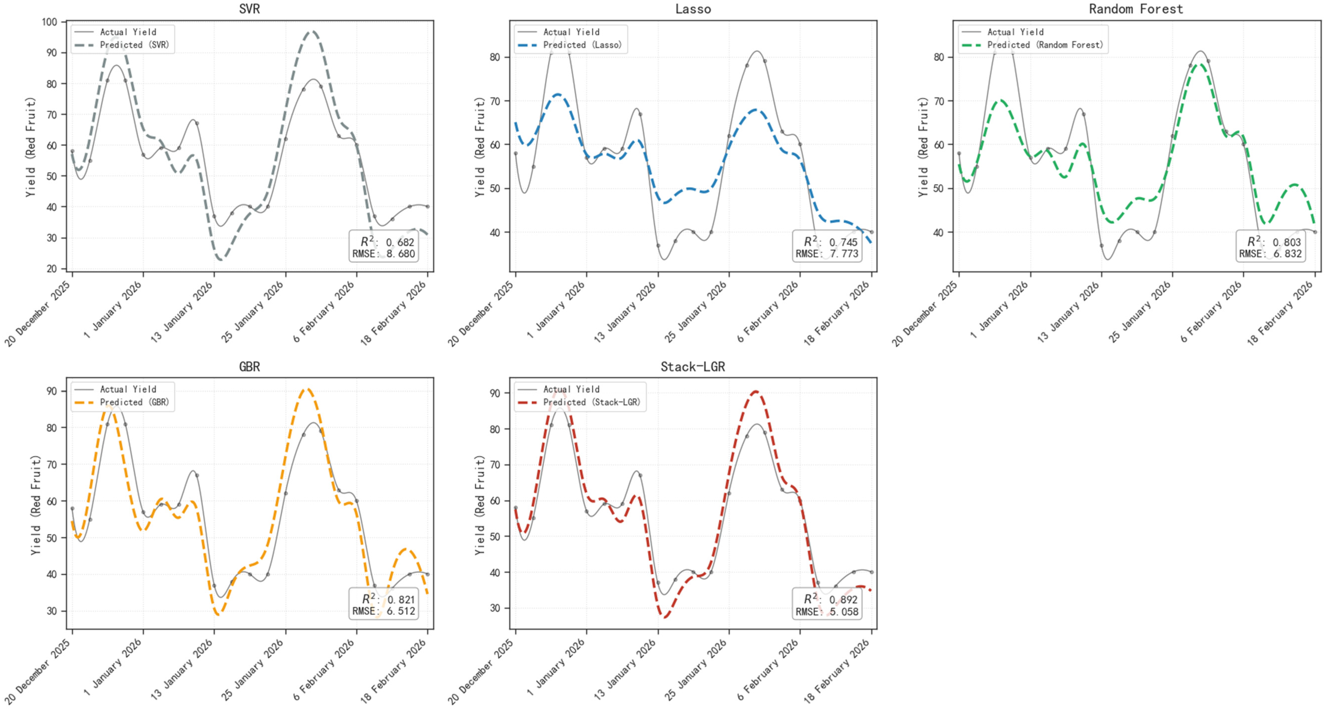
To comprehensively evaluate the effectiveness of the proposed two-layer ensemble architecture for short-term strawberry yield prediction, we conducted a comparison against its constituent base learners (Lasso regression and gradient boosting regression, GBR) alongside traditional machine learning baselines (support vector regression, SVR, and Random Forest, RF), as illustrated in Figure 15. The evaluation metrics adopted for this assessment include the coefficient of determination ($R^2$), root mean square error (RMSE), and Mean Absolute Error (MAE), where both RMSE and MAE are expressed in units of fruit per plant (fruit/plant). Their respective calculation formulas are defined in Equations (15)–(17). The quantitative experimental results of this comparative analysis are comprehensively summarized in

Table 5. Comparison of yield prediction performance among different prediction models.

Model	R2	RMSE	MAE
SVR	0.682	8.680	7.205
Lasso Regression	0.745	7.773	6.042
Random Forest	0.803	6.832	5.642
GBR	0.821	6.512	5.185
Stack-LGR	0.892	5.058	3.865

.

$$R^2=1-{\displaystyle \frac{{\sum }_{i=1}^n{\left(y_i-\widehat{y_i}\right)}^2}{{\sum }_{i=1}^n{\left(y_i-\overline{y}\right)}^2}}$$

(15)

$$RMSE=\sqrt{{\displaystyle \frac{1}{n}}\sum _{i=1}^n{\left(y_i-\widehat{y_i}\right)}^2}$$

(16)

$$MAE={\displaystyle \frac{1}{n}}\sum _{i=1}^n\left|y_i-\widehat{y_i}\right|$$

(17)

The experimental results indicate that the proposed Stack-LGR architecture significantly outperforms all comparative models across the evaluated metrics. Specifically, when compared to the best-performing individual base learner (GBR), the Stack-LGR model achieves a superior $R^2$ of 0.892, alongside substantial reductions in RMSE (by 22.3%, from 6.512 to 5.058) and MAE (by 25.5%, from 5.185 to 3.865). Furthermore, when benchmarked against the Lasso model—which is intrinsically constrained to linear feature selection—the generalization superiority of the ensemble approach becomes even more pronounced, evidenced by an approximate 19.7% increase in $R^2$ and a 34.9% decrease in RMSE.

This significant performance gain is primarily attributed to the Stack-LGR model’s capacity to synergistically fuse the decision boundaries of its heterogeneous base learners. Traditional standalone models often struggle to capture the complex dynamics of greenhouse environments. For instance, linear models such as Lasso struggle to capture the highly nonlinear impacts of meteorological factors—such as sudden diurnal temperature shifts and the nonlinear progression of effective accumulated temperature (GDD)—on strawberry yield. Conversely, while tree-based algorithms like GBR and RF possess stable nonlinear fitting capabilities, they remain highly susceptible to overfitting induced by localized data noise and transient microclimate anomalies.

By introducing a ridge regression model with $L_2$ regularization constraints as the meta-learner (Level-1), the architecture dynamically redistributes global weights between the linear baseline trends and the nonlinear residual fluctuations extracted by the base learners. This secondary calibration mechanism not only effectively suppresses the prediction bias inherent to individual base learners but also synergistically utilizes their complementary feature representations. Ultimately, when confronted with high-dimensional, non-stationary meteorologically driven time series, the model can stably capture the crop’s growth inertia while smoothing out errors induced by local environmental disturbances. This effectively mitigates the generalization bottlenecks that plague traditional standalone models in complex, nonlinear agricultural systems.

3.2.2. Stability Analysis of Stack-LGR via Five-Fold Cross-Validation

To evaluate the robustness and generalization of the proposed Stack-LGR model, a 5-fold cross-validation (CV) was conducted, as shown in

Table 6. Five-fold cross-validation results of the Stack-LGR model.

Fold	R2	RMSE	MAE
Flod1	0.887	5.132	3.902
Flod2	0.895	5.041	3.854
Flod3	0.890	5.089	3.873
Flod4	0.899	4.976	3.821
Flod5	0.889	5.072	3.872
Mean ± Std	0.892 ± 0.004	5.062 ± 0.058	3.865 ± 0.028

. The dataset was partitioned into five mutually exclusive subsets at the plant level. All temporal samples derived from the same strawberry plant were assigned exclusively to the same subset to prevent potential information leakage caused by overlapping temporal windows. In each fold, four subsets of strawberry plants were used for model training, while the remaining subset was used for testing. This process was repeated five times so that each subset served once as the test set.

The experimental results demonstrate that the Stack-LGR model exhibits relatively stable performance across different data partitions. Specifically, the R² values range from 0.887 to 0.899, with a mean value of 0.892 ± 0.004. The RMSE values vary from 4.976 to 5.132, yielding an average of 5.062 ± 0.058. Similarly, the MAE values range from 3.821 to 3.902, with a mean of 3.865 ± 0.028. These results indicate that the proposed model maintains consistent predictive performance under different training–testing splits.

Overall, the low standard deviations across all evaluation metrics confirm that the Stack-LGR model is relatively stable and not overly sensitive to data partitioning. This further demonstrates its robustness and reliability in yield prediction tasks under limited-sample conditions.

3.2.3. Feature Contribution and Interpretability Analysis

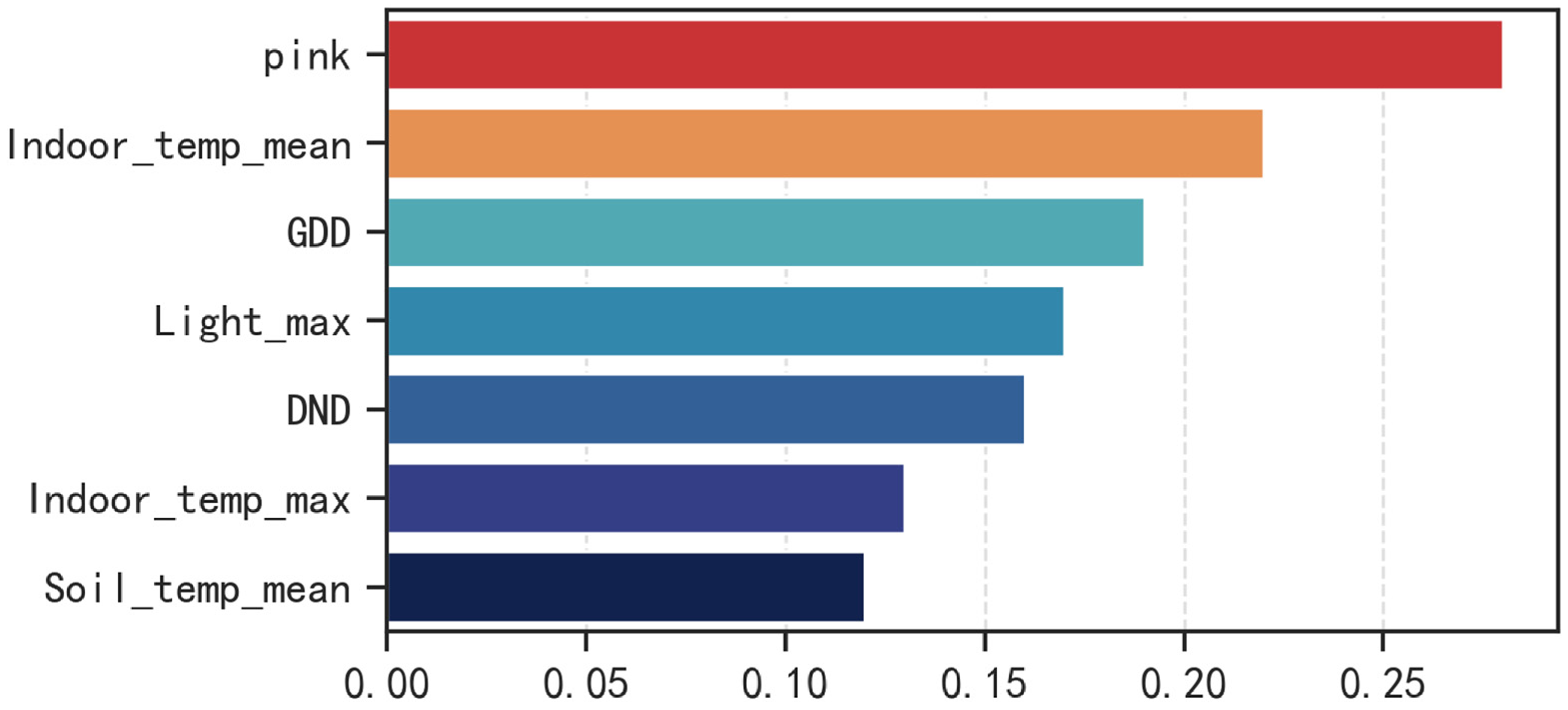
To elucidate the underlying agronomic rationale of the Stack-LGR model’s internal decision-making mechanics, we extracted the standardized weight contributions of each input feature within the Level-1 ridge meta-learner, as illustrated in Figure 16. The results indicate that the architecture not only achieves stable predictive accuracy from an algorithmic perspective but also exhibits a feature weight distribution that closely aligns with the actual phenological progression and growth dynamics of strawberries in controlled greenhouse environments.

As shown in Figure 16, the feature weight distribution within the model aligns closely with the agronomic mechanisms governing short-term yield formation over the $T+1$ to $T+3$ prediction window. Notably, the computer-vision-extracted pink fruit count (contribution weight: 0.28) dominates the feature importance hierarchy. As the direct biological precursor to harvestable red fruits, it firmly anchors the static physiological baseline for potential yield. Indoor average temperature (0.22) and effective accumulated temperature follow closely, accurately reflecting the physiological thermal engine required to drive rapid fruit coloration and ripening. Concurrently, solar irradiance and diurnal temperature amplitude are assigned proportional weights, representing the nonlinear regulation of dry matter accumulation and fruit quality by light-temperature synergy. Conversely, soil temperature receives diminished weight in this short-term prediction context due to its pronounced temporal lag effect on phenotypic progression, functioning primarily as a background constraint on basal metabolism. In summary, the Stack-LGR deconstructs the hidden internal decision mechanisms of machine learning, autonomously constructing a physiologically interpretable logic that is centered on pink fruit reserves, driven by thermal accumulation, and dynamically regulated by microclimatic synergy.

3.2.4. Spatial Distribution of Errors and Residual Diagnosis

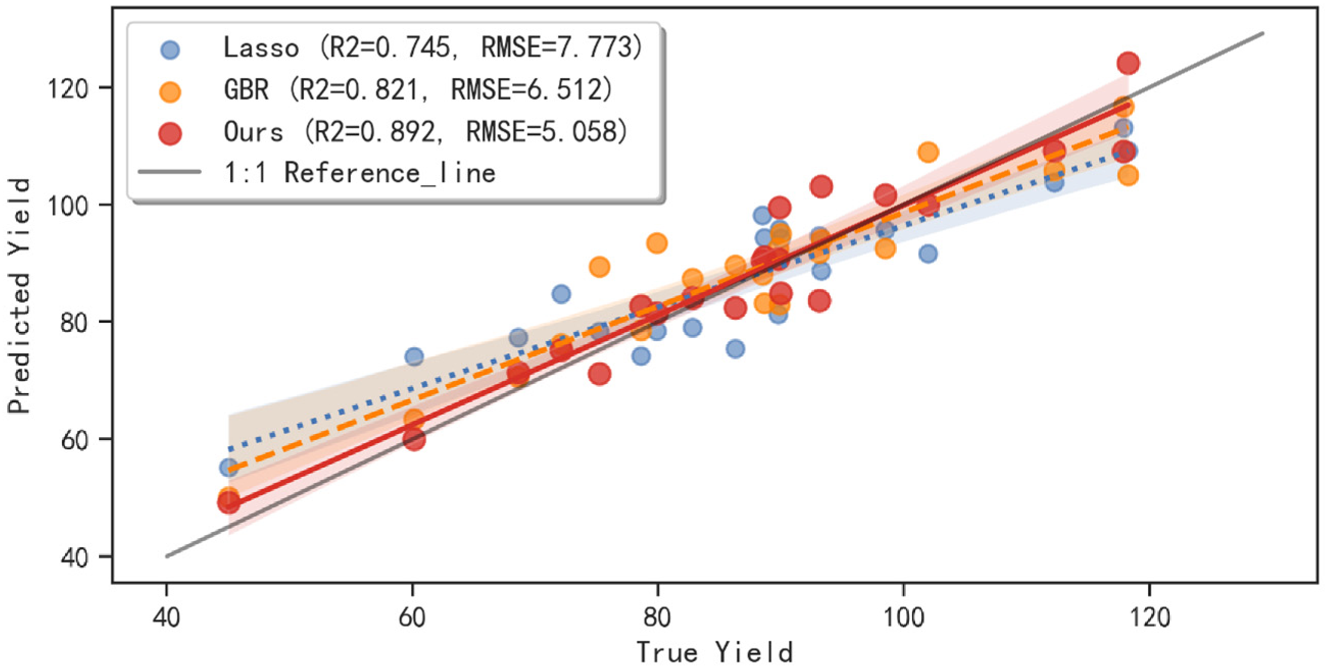
To visually assess the predictive stability of the different models across various yield ranges, scatter plots of predicted versus observed values were generated for the individual base learners (Lasso, GBR) and the proposed Stack-LGR model using the validation set, as illustrated in Figure 17. The solid black line in the figure represents the 1:1 identity line. The closer the fitted regression line aligns with this reference line, and the tighter the clustering of data points around it, the higher the model’s predictive accuracy and the lower its inherent bias.

As evidenced by the scatter plots and error distributions in Figure 17, the proposed Stack-LGR architecture ($R^2$ = 0.892, RMSE = 5.058) demonstrates the highest predictive stability. Its predicted distribution closely adheres to the 1:1 identity line, successfully overcoming the structural limitations inherent to standalone baselines. Specifically, the Lasso model ($R^2$ = 0.745), strictly constrained by linear assumptions, exhibits pronounced systematic bias at the yield extremes—overestimating low yields and underestimating high yields. Conversely, while the GBR model ($R^2$ = 0.821) improves nonlinear mapping, it remains susceptible to high-frequency meteorological noise, leading to greater predictive variance. The exceptional generalization capability of the Stack-LGR ensemble is primarily attributed to its two-layer reconstruction mechanism. The Level-0 heterogeneous base learners decouple the linear growth inertia from nonlinear climatic disturbances, whereas the Level-1 ridge meta-learner executes a global $L_2$-regularized weight calibration to rectify base-level prediction biases. This synergistic mechanism effectively neutralizes the systematic errors typical of individual models and smooths out local microclimatic noise, ultimately delivering high-precision, unbiased predictions across the entire yield spectrum.

3.3. Deep Learning-Based High-Precision Yield Prediction Methods

3.3.1. Performance Evaluation and Comparison of the BiTCN-SA Model

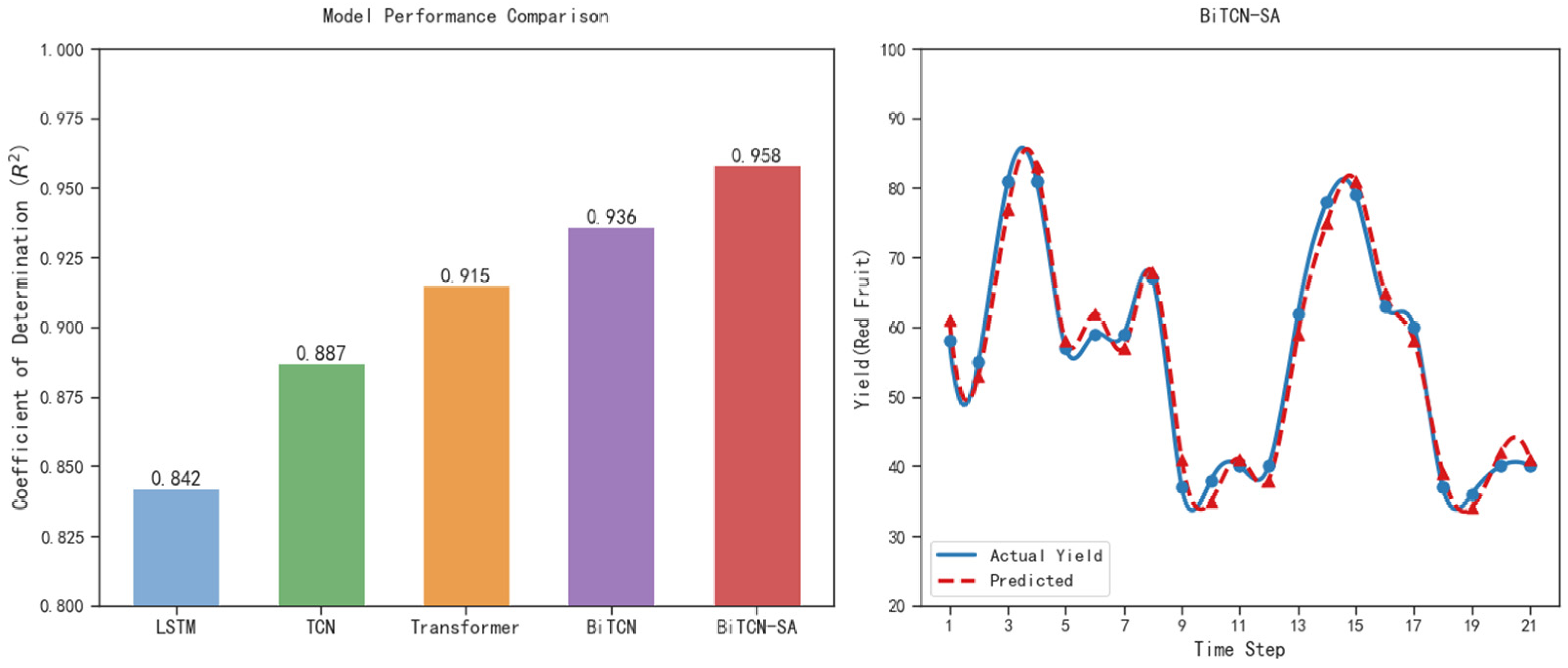
To rigorously evaluate the predictive efficacy of the proposed BiTCN-SA model for short-term strawberry yield prediction (i.e., for the next harvesting cycle), we conducted a systematic comparison against standard baseline models, including LSTM, TCN, Transformer, and the basic BiTCN. As illustrated in Figure 18 and summarized in

Table 7. Comparison of yield prediction performance among deep learning models.

Model	R2	RMSE	MAE
LSTM	0.842	6.118	4.350
TCN	0.887	5.174	3.831
Transformer	0.915	4.488	3.276
BiTCN	0.936	3.894	2.685
BiTCN-SA	0.958	3.154	2.049

, the input for all evaluated models consisted of identically constructed multivariate meteorological–phenological time-series sequences $X\in R^{T\times C}$. These sequences encompass critical meteorological statistics (averages, maximums, and minimums) alongside key agronomic indices such as effective accumulated temperature (GDD) and diurnal temperature differences (DNDs).

The experimental results indicate that the standard LSTM baseline yields suboptimal performance compared to the other evaluated deep learning architectures ($R^2$ = 0.842, RMSE = 4.350). Mechanistically, this underperformance is attributed to the complex nature of strawberry yield, which is synergistically driven by both prolonged meteorological trends and transient extreme weather events. The unidirectional nature of the LSTM’s gating mechanism makes it highly susceptible to progressive information attenuation when processing extended temporal sequences. Consequently, it struggles to accurately capture sudden, short-term nonlinear microclimatic fluctuations, ultimately justifying the need to replace standard LSTM models with more advanced BiTCN architectures.

In contrast, the TCN architecture, which is based on causal dilated convolutions ($R^2$ = 0.887), effectively mitigates the progressive information attenuation inherent to the standard LSTM baseline. By expanding the receptive field and incorporating residual connections, the TCN achieves a 15.4% reduction in RMSE compared to the LSTM. However, because the TCN relies exclusively on unidirectional historical data, it fails to fully exploit the backward contextual constraints provided by meteorological data from the next harvesting period. Notably, the Transformer model, relying purely on global self-attention mechanisms, demonstrates highly competitive performance ($R^2$ = 0.915). By computing parallel attention across the entire sequence, it significantly outperforms the unidirectional TCN at modeling global feature interactions. Nevertheless, due to the Transformer’s inherent lack of inductive bias for local temporal dynamics (e.g., an abrupt temperature drop over two consecutive days), it remains inadequate in capturing the strict localized temporal continuity of strawberry growth.

By introducing a bidirectional temporal convolutional branch, the baseline BiTCN architecture ($R^2$ = 0.936) seamlessly synthesizes the cumulative biological inertia of past growth with the retroactive environmental constraints of future weather predictions. This integration achieves error metrics that are significantly lower than those of both the Transformer and the unidirectional TCN. Building upon this stable foundation, the proposed BiTCN-SA model delivers superior predictive accuracy, registering an unprecedented $R^2$ of 0.958 while driving RMSE and MAE down to optimal minimums of 3.154 and 2.049, respectively. When benchmarked against the standalone BiTCN without the attention mechanism, the RMSE is reduced by an additional 19%. From a mechanistic perspective, this substantial improvement proves that the self-attention module effectively mitigates the inherent inflexibility of static convolutional kernels. It empowers the network to adaptively allocate attention weights to critical temporal junctures that trigger severe yield volatility—specifically, anomalous shifts in effective accumulated temperature (GDD) or diurnal temperature differences (DND). Consequently, the BiTCN-SA architecture achieves maximum predictive fidelity and stability within highly complex, coupled agrometeorological environments.

3.3.2. Stability Analysis of BiTCN-SA via Five-Fold Cross-Validation

To assess whether the BiTCN-SA model suffered from overfitting and to further evaluate its robustness and generalization capability, a 5-fold cross-validation experiment was conducted, as shown in

Table 8. Five-fold cross-validation results of the BiTCN-SA model.

Fold	R2	RMSE	MAE
Flod1	0.952	3.232	2.074
Flod2	0.963	3.086	2.028
Flod3	0.956	3.178	2.060
Flod4	0.965	3.071	2.018
Flod5	0.955	3.203	2.067
Mean ± Std	0.958 ± 0.005	3.154 ± 0.047	2.049 ± 0.017

. The dataset was partitioned into five mutually exclusive subsets at the plant level. All temporal samples generated from the same strawberry plant were assigned exclusively to the same subset to prevent information leakage caused by overlapping temporal windows. In each fold, four subsets of plants were used for model training, while the remaining subset was used for testing. This process was repeated five times so that each subset served once as the test set.

The experimental results demonstrate stable performance across all folds. Specifically, the R² values range from 0.952 to 0.965, with a mean of 0.958 ± 0.005. The RMSE values vary from 3.071 to 3.232, yielding an average of 3.154 ± 0.065. Similarly, the MAE values range from 2.018 to 2.074, with a mean of 2.049 ± 0.024. These results indicate that the proposed BiTCN-SA model maintains consistent predictive performance across different data partitions.

Overall, the low standard deviation across all evaluation metrics confirms the model’s stability and robustness, suggesting that the BiTCN-SA framework is not highly sensitive to data splitting and exhibits strong generalization under limited-sample conditions.

3.3.3. Discussion of Model Decision Mechanisms and Attention Visualization Analysis

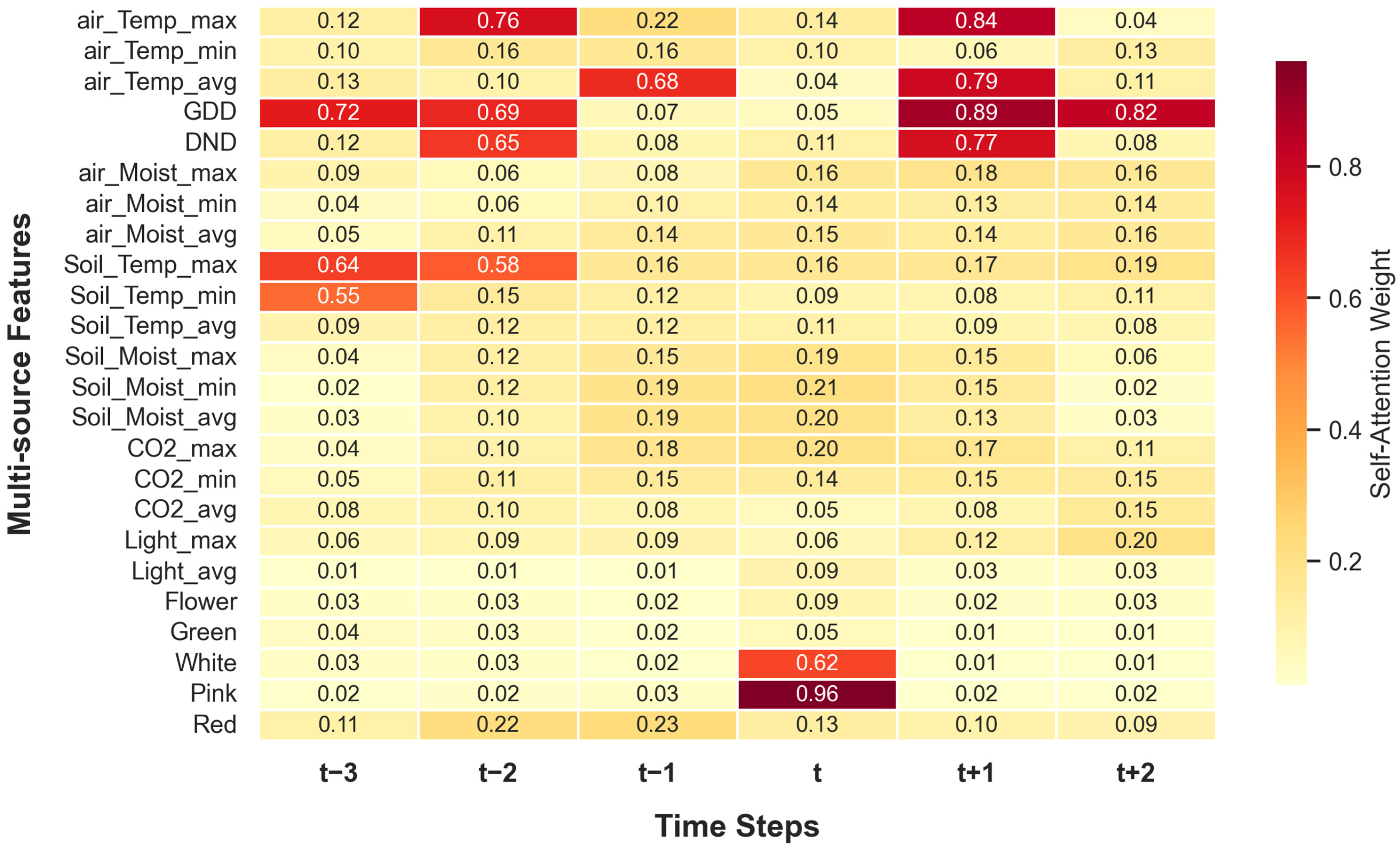
In practical agricultural applications, deep learning models often lack decision transparency due to their inherent opacity. To verify whether the proposed BiTCN-SA model genuinely captures the underlying mechanistic relationships linking meteorological drivers to strawberry phenological development, we extracted self-attention weight distributions from test-set samples during the short-term yield prediction phase. As illustrated in Figure 19, these dynamic weight allocations were subsequently visualized as feature-temporal attention heatmaps.

The self-attention weight matrix clearly reveals that the BiTCN-SA model has autonomously identified the primary drivers of short-term strawberry yield. First, among the visual phenotypes inputted at a static temporal juncture, the network allocates peak attention weights (reaching 0.96) to the inventory of pink fruits at the current day ($t$). This data-driven focus perfectly corroborates the established objective phenological trajectory, whereby pink fruits systematically transition to the mature red stage within a 1-to-3-day window.

Second, within the meteorological environment matrix, the model exhibits pronounced sensitivity to specific microclimatic indicators. As illustrated in Figure 19, the network assigns relatively higher weights to Air Temperature, Growing Degree Days (GDDs), and diurnal temperature differences (DNDs) within the observed meteorological sequence, indicating that these variables play dominant roles in characterizing short-term strawberry yield dynamics. Meanwhile, root-zone soil temperature receives greater attention during the preceding lag phase, reflecting its contribution to the accumulation of thermal conditions during earlier growth stages. Mechanistically, this weight distribution suggests that the network successfully captures the environmental coupling relationships underlying strawberry ripening processes. Specifically, the model integrates three critical components: historical root-zone thermal conditions, the current inventory of transitional (pink) fruits, and observed meteorological variations associated with thermal accumulation and diurnal temperature fluctuations. Together, these factors provide complementary information for explaining the short-term transition from immature and transitional fruits to harvestable red fruit yield.

3.4. Comprehensive Comparison and Discussion of the Applicability of Machine Learning and Deep Learning Prediction Methods

To comprehensively evaluate multi-source data-driven solutions for short-term strawberry yield prediction, this section provides a systematic comparative analysis of the proposed machine learning ensemble (Stack-LGR) and the deep learning architecture (BiTCN-SA). As detailed in

Table 9. Performance comparison between the proposed BiTCN-SA and the baseline Stack-LGR model.

Metrics	Stack-LGR	BiTCN-SA
$R^2$	0.892	0.958
RMSE	5.058	3.154
MAE	3.865	2.049
Feature extraction	Manual engineering	Automated coupling
Model size	27 KB	1.3 MB
Computational cost	49K FLOPs	4M FLOPs

, this comparison evaluates predictive efficacy, inherent feature discovery mechanisms, and the potential for practical agricultural deployment.

In terms of overall prediction accuracy, the deep learning model BiTCN-SA exhibits a pronounced advantage ($R^2$ = 0.958, representing a 6.6% improvement over the Stack-LGR ensemble). This significant performance gap stems primarily from fundamental differences in how the two architectures process multivariate meteorological time series. Although the machine learning Stack-LGR architecture significantly mitigates the generalization error of individual base learners through multi-model fusion, thereby establishing a stable predictive baseline (RMSE = 5.058), it remains inherently reliant on hand-crafted feature engineering. Consequently, when confronted with highly volatile meteorological environments (e.g., extreme Day–Night Temperature Differences, DNDs) and complex visual phenological data, the traditional machine learning paradigm struggles to autonomously extract nonlinear, dynamic coupling relationships across extended temporal horizons. In stark contrast, the BiTCN-SA architecture, leveraging dilated causal convolutions, natively processes high-dimensional matrix inputs. It demonstrates a sensitivity that far surpasses that of statistical models when fitting the extreme nonlinear trajectories associated with strawberries entering exponential red fruit burst phases or experiencing cold-stress-induced developmental stagnation.

Regarding agronomic interpretability and response mechanisms, the two methodological paradigms exhibit distinct focuses. Machine learning architectures, such as the ensemble of the tree-based GBR and linear Lasso models, excel at capturing immediate environmental stimuli and offer intrinsic interpretability through explicit feature importance rankings. However, the maturation of non-climacteric fruits, such as strawberries, is fundamentally driven by prior thermal accumulation and exhibits pronounced meteorological lag effects. The bidirectional temporal convolutions within the BiTCN-SA architecture not only seamlessly integrate historical growth states (e.g., accumulated photosynthetic assimilation) with retroactive meteorological data from the next harvesting period constraints, but also actively demystify the inherent opacity of traditional deep learning through its self-attention mechanism. As evidenced by the preceding heatmaps, the BiTCN-SA autonomously focuses on the Growing Degree Days (GDDs) from three days prior ($t-3$) and the transitional white and pink fruit counts from the preceding day ($t-1$). This automated attention allocation along the phenological progression ladder represents a profound level of deep feature representation that remains fundamentally unattainable by traditional machine learning methodologies.

In real-world smart agriculture deployments, computational overhead and hardware constraints are critical factors that determine a model’s practical applicability. A quantitative complexity analysis reveals that the BiTCN-SA architecture—integrating bidirectional temporal convolutions and dual-path self-attention—contains approximately $3.2\times {10}^5$ trainable parameters. Considering the relatively limited dataset size in this study, which consisted of observations collected from 150 individual strawberry plants, the potential risk of overfitting was carefully considered. To assess the generalization capability and evaluate potential overfitting, a five-fold cross-validation (CV) experiment was conducted. As shown in Table 8, the BiTCN-SA model achieved stable performance across all validation folds, with an average $R^2$ of 0.958 ± 0.005, RMSE of 3.154 ± 0.047, and MAE of 2.049 ± 0.017. The low variability among different folds indicates that the model maintained consistent predictive performance despite its relatively complex architecture. Although this sophisticated architecture provides strong nonlinear feature representation capability and enhances predictive accuracy, a single inference step incurs a computational cost of approximately 4 MFLOPs. This computational burden is primarily attributed to the matrix dot-product operations involved in the self-attention mechanism and the dense computations associated with high-dimensional convolutional kernels. Consequently, this deep learning framework requires hardware acceleration (e.g., GPU support) and is more suitable for deployment on server platforms with sufficient computational resources.

In stark contrast, the proposed Stack-LGR framework exhibits a highly lightweight computational footprint. By integrating shallow decision trees in the Gradient Boosting Regression component with sparse linear regression models, the model is overall highly efficient in terms of computation. For the complete dataset collected from 150 individual strawberry plants across 22 harvesting cycles, the total computational cost is approximately 4.9 × 10⁴ FLOPs. Overall, the proposed framework achieves a strong balance between predictive performance and computational efficiency, making it well-suited for low-sample, resource-constrained scenarios. The reduced computational demand lowers hardware requirements and enhances deployment feasibility in edge-computing-based agricultural IoT systems. Even in decentralized greenhouse environments with limited computing power or unstable network connectivity, the model can still provide stable, real-time yield predictions, enabling timely decision-making.

In summary, rather than being mutually exclusive, machine learning and deep learning represent highly complementary methodological paradigms for yield estimation tasks in modern controlled-environment agriculture. The BiTCN-SA architecture establishes the ultimate predictive ceiling when processing high-dimensional, multi-source data streams. Conversely, the Stack-LGR ensemble enables stable baseline reliability and operational feasibility across complex, resource-constrained deployment environments.

3.5. Analysis of Multimodal Fusion Effectiveness

To validate the necessity of the multimodal fusion strategy, we conducted rigorous modality ablation experiments to compare the model’s predictive performance across various input combinations. For the phenological data, fruit developmental information was quantified as numerical features by recording the number of fruits at different growth stages (flower, green, white, pink, and red). These numerical representations were subsequently used as inputs for model training and prediction. As shown in Figure 20, the predictive performance was evaluated under four input configurations: meteorological data only, pink fruit count only, phenological data only, and the integrated meteorological–phenological fusion strategy.

The results indicate that different modalities provide complementary information for yield prediction. When only meteorological data were used, the predictive performance was relatively limited, with $R^2$ values of 0.605 for Stack-LGR and 0.671 for BiTCN-SA, suggesting that environmental variables alone may not sufficiently describe the physiological development process of strawberry plants. The pink fruit-only input achieved higher predictive performance, with $R^2$ values of 0.698 and 0.742 for Stack-LGR and BiTCN-SA, respectively, indicating that fruit developmental status provides useful information for yield estimation. However, a single phenological indicator may not fully represent the complex developmental characteristics of strawberry plants.

When the complete phenological information was incorporated, the $R^2$ values increased to 0.759 for Stack-LGR and 0.813 for BiTCN-SA, suggesting that multi-dimensional phenological features can provide a more comprehensive representation of fruit development compared with a single indicator. Furthermore, combining meteorological and phenological information further improved the prediction performance of BiTCN-SA, with the $R^2$ value increasing from 0.813 under the phenology-only condition to 0.958 under the multimodal fusion condition. This result indicates that meteorological information can provide additional environmental context and contribute to capturing the dynamic changes associated with strawberry ripening and yield formation.

From the perspective of model architecture, BiTCN-SA consistently achieved higher $R^2$ values than Stack-LGR under all input configurations, indicating its potential advantage in extracting nonlinear relationships and integrating multi-source information. Under the multimodal fusion condition, BiTCN-SA achieved an $R^2$ value of 0.958, compared with 0.892 for Stack-LGR, suggesting that the proposed temporal attention-based framework is effective in modeling the interactions between phenological development and environmental factors. Overall, the integration of phenological and meteorological information provides complementary features for short-term greenhouse strawberry yield prediction, while BiTCN-SA offers an effective approach for utilizing these multi-source data.

4. Discussion

To further validate the effectiveness and validity of the PRED-VPMS method proposed in this study, we have categorized existing research on short-term yield prediction for greenhouse strawberries and related cash crops into three major technical approaches for systematic evaluation. By quantitatively comparing their algorithmic mechanisms, achieved results, and prediction accuracy, we thoroughly examine the technical bottlenecks of each approach and highlight the breakthroughs of this study.

4.1. Vision-Only Yield Prediction

In vision-only yield prediction, researchers primarily rely on computer vision (CV) techniques. By performing high-precision detection, segmentation, and dynamic counting of strawberry organs such as flowers and fruits in images, they infer current yield potential based on the physical fruit load.

In complex environments, to address yield estimation errors caused by dense overlapping and severe occlusion in greenhouses, Li et al. [35] proposed the YOLOv5-ASFF algorithm based on adaptive spatial feature fusion, which achieved an average precision (AP) of up to 98.77% for strawberries at maturity. Regarding more refined pixel-level instance segmentation, Ghose et al. [36] combined YOLO with the Segment-Anything (SAM) large model to achieve precise extraction of strawberry fruits in complex backgrounds under few-shot learning conditions, achieving a Dice coefficient of 0.95. In the realm of dynamic tracking and deduplication counting, to address the issue of overestimated yields caused by duplicate counts in video streams or continuous sampling, Vaishnavi et al. [37] utilized Mask R-CNN combined with the Deep SORT multi-object tracking algorithm, maintaining a true physical count accuracy of 92.3% in dense canopies; Wang et al. [38] introduced a region-based tracking algorithm into greenhouse tomato yield estimation using a lightweight YOLO11n model, successfully reducing the mean counting error (MCE) to 6.6%. In edge computing research, the RTF-YOLO model developed by Shen et al. [39] maintained a mean average precision (mAP) of 90.24% while ensuring ultra-fast inference. Furthermore, Aldakn et al. [40] utilized YOLOv12 in conjunction with drone imagery to not only achieve target counting but also directly construct a nonlinear regression mapping from fruit geometric dimensions to weight, with a coefficient of determination ($R^2$) as high as 0.99 and an absolute error in weight estimation as low as 2.9–5%.

Although current vision-only models have achieved extremely high accuracy in estimating static fruit inventory, the core limitation of this approach is that its output reflects only a static physical snapshot of the crop. Simple computer vision algorithms cannot dynamically perceive environmental variables. They cannot predict how sudden changes in temperature and humidity over the coming days will accelerate or inhibit the fruit ripening cycle. In contrast, while the YOLO11-SC model in this study improves feature extraction capabilities by introducing a dual attention mechanism (SE+CBAM), it is not designed as an end-to-end yield estimation model at the system architecture level. We perform feature dimensionality reduction on the high-weighted counts of pink and white fruits extracted from visual data, converting them into static baselines that characterize the plant’s developmental potential, and feed these into downstream temporal networks (Stack-LGR and BiTCN-SA) for processing. This design mitigates the limitation of vision-only models, which capture only current stock but cannot predict future conversion rates. It lays the foundation for subsequent meteorology-driven multimodal temporal prediction.

4.2. Yield Prediction Using Only Meteorological Environmental Sequences

Yield prediction using only meteorological environmental sequences eliminates the need for image-based phenotyping, instead focusing on in-depth analysis of microclimate indicators—such as light, temperature, water, and air—or energy input sequences within the greenhouse. It employs only data-driven algorithms to fit the nonlinear mapping between environmental trends and final yield.

To address the complexity of greenhouse microclimate fluctuations, Yamazaki et al. [41] employed a generalized additive model (GAM) to perform nonparametric statistical regression on temporal features such as diurnal temperature range. While they managed to keep the mean absolute percentage error (MAPE) at 0.18 within a stationary period, their adjusted coefficient of determination (R²) was only 0.72, making it difficult to effectively cope with sudden environmental stresses. Recognizing the significant noise present in instantaneous meteorological data, some researchers introduced cumulative energy metrics. Alvarado et al. [42] quantitatively assessed the effective accumulated temperature (GDD) for strawberries at different phenological stages. They found a very high positive correlation (r > 0.9) between GDD and the developmental progress of strawberry flowering and fruiting, thereby confirming the scientific value of cumulative energy metrics. When handling complex, long-term microclimate time series, Li et al. [43] used Long Short-Term Memory (LSTM) networks to estimate yield for greenhouse crops. Although this approach effectively captured the lag effects of meteorological factors, its root mean square error (RMSE) still showed significant fluctuations during sudden extreme temperature changes. Addressing the high dimensionality and nonlinearity of microclimate data, Liu et al. [44] further demonstrated that Time Convolutional Networks (TCNs) offer significant advantages for identifying high-frequency environmental fluctuations.

Despite continuous iterations of only meteorological models, they struggle to capture the actual fruit-bearing stock of the crop, thereby inevitably introducing systematic errors. In their study on the relationship between strawberry yield and meteorological conditions, VC et al. [45] explicitly highlighted the theoretical challenge of “same temperature, different effects” from an agro-meteorological perspective: maximum temperature shows a significant positive correlation with yield from strawberry planting to the early stage of inflorescence emergence, but the same maximum temperature exhibits a significant negative correlation with yield from flowering to fruit set. This implies that, if a model lacks visual phenological information (i.e., the current developmental stage of the strawberry plants), it cannot accurately assess the true catalytic or inhibitory effects of current meteorological conditions on final yield. Due to a lack of awareness of the plants’ actual fruit-bearing status, only meteorological models—even those employing deep LSTM or TCN architectures—are prone to reaching their inherent upper limits of predictive accuracy.

4.3. Yield Prediction by Integrating Visual Images and Meteorological Data

The multimodal fusion approach represents the cutting edge of yield estimation in smart agriculture, aiming to simultaneously leverage the synergistic effects of image-based phenological perception and meteorological time-series insights to overcome the accuracy bottlenecks of single-modal methods.

In the realm of multimodal fusion, Shamsuddin et al. [46] demonstrated that a DNN model incorporating intermediate-layer multimodal feature fusion (R² = 0.73) that integrates RGB images, crop phenotypes, and microclimate data significantly outperforms single-modal networks. To prevent the loss of visual features during fusion, Mia et al. [47] used CNNs to extract canopy-image features. They integrated them with weekly meteorological time series, effectively improving the lower bound of yield estimation in complex field environments. Cutting-edge research is increasingly focusing on the temporal asymmetry of fused data. Jiang et al. [48] noted that “post-image weather” conditions following the capture of visual snapshots can significantly affect the final yield. To address this, the UAV framework they developed explicitly accounted for meteorological sequences following image acquisition, successfully increasing the coefficient of determination ($R^2$) to 0.61. PhenoYieldNet, developed by Luo et al. [49], further demonstrated that modeling how meteorological drivers dynamically regulate specific phenological stages is essential to address complex nonlinear agricultural habitats. Furthermore, to address the curse of dimensionality caused by high-dimensional heterogeneous features, Yewle et al. [50] developed the RicEns-Net deep ensemble learning framework, which validated the strong stability of multiple machine learning-based classifiers in yield estimation through multi-source data fusion.

Although existing multimodal studies [46,47,48,49,50] have demonstrated the effectiveness of integrating heterogeneous agricultural data sources, such as remote sensing imagery, meteorological variables, and environmental factors, their reported performances should be interpreted considering differences in dataset characteristics, prediction objectives, and evaluation protocols. Most existing approaches rely on feature-level fusion or static temporal alignment strategies, where visual observations and environmental variables are generally treated as concurrent inputs. However, crop yield formation is a dynamic physiological process involving delayed responses between environmental stimuli and fruit maturation. Therefore, such fusion strategies may have limited capability in capturing meteorological lag effects caused by cumulative thermal conditions and short-term climatic fluctuations. Moreover, differences in crop species, cultivation environments, sampling intervals, prediction horizons, and validation strategies may also contribute to the variation in reported performance among different studies.

The relatively lower prediction performance reported in some previous studies may be attributed to several factors. First, many existing multimodal frameworks were developed for field-scale crop yield estimation, where environmental heterogeneity and irregular sampling conditions introduce additional uncertainties. Second, image and meteorological information were often aligned according to the same observation time, limiting the ability of these models to characterize future yield conversion processes. Third, some approaches employ general feature fusion mechanisms without explicitly incorporating crop phenological states as physiological constraints. Consequently, although multimodal learning improves information utilization, the absence of explicit physiological guidance may restrict the model’s ability to interpret how environmental changes influence fruit development at different growth stages.

In comparison, the proposed PRED-VPMS framework differs from previous studies in both feature representation and temporal modeling strategies. Rather than treating visual and meteorological information as synchronous independent features, this study introduces a phenology-guided temporal fusion mechanism. Specifically, the five-dimensional phenological vector extracted by YOLO11-SC provides the current physiological baseline of strawberry plants, while the six-day bidirectional meteorological window captures both historical growth accumulation effects and future environmental regulation. This design enables the model to better characterize the delayed relationship between meteorological variations and fruit maturation, thereby overcoming the limitations of vision-only models that only reflect current fruit inventory and meteorology-only models that lack awareness of crop physiological states.

Furthermore, the proposed dual-deployment architecture provides flexibility for different agricultural computing scenarios. For server-side applications with sufficient computational resources, the BiTCN-SA model utilizes bidirectional temporal convolution and self-attention mechanisms to capture complex spatiotemporal dependencies among meteorological variations and phenological distributions, achieving an R² value of 0.958. For resource-constrained agricultural IoT edge devices, the Stack-LGR lightweight architecture provides an efficient alternative. By combining heterogeneous base learners with two-layer regularization, Stack-LGR effectively reduces the influence of local meteorological noise and achieves stable prediction performance (R² = 0.892) with only approximately 49K FLOPs during inference. These results demonstrate that the proposed framework not only improves prediction accuracy through effective multimodal temporal fusion but also provides practical deployment flexibility under heterogeneous hardware conditions.

5. Conclusions

To address industry pain points, such as the challenges of short-term yield prediction and delayed meteorological responses in modern protected strawberry production, we proposed and validated a short-term yield prediction method for greenhouse strawberries that integrates visual phenology and meteorological sequences. First, by optimizing the YOLO11 object detection network with the introduction of attention mechanisms, we effectively overcame the challenge of fruit occlusion in complex greenhouse environments, achieving high-precision automated extraction of five consecutive strawberry phenological stages. The deep fusion of these visual phenological features with meteorological sequences constructed a highly valuable high-dimensional spatiotemporal feature matrix for downstream prediction. Based on this feature engineering, our designed BiTCN-SA deep learning model demonstrated strong performance in predicting red fruit yield within the next harvesting cycle ($R^2$ = 0.958, RMSE = 3.154), successfully corroborating the synergistic developmental laws of early thermal accumulation drives and the recent transition from pink/white to red fruit at the biological mechanism level. Furthermore, considering the practical deployment needs of smart agriculture, systematic evaluation confirmed that the high-precision BiTCN-SA model is suitable for server platforms with ample computational resources. Meanwhile, the synchronously constructed Stack-LGR model, owing to its extremely low computational complexity and strong anti-overfitting stability, provides a reliable, lightweight alternative for resource-constrained agricultural Internet of Things (IoT) edge devices. In summary, our research resolved the challenge of short-term agricultural multi-source data fusion for yield prediction at the algorithmic level, providing decision support for just-in-time harvest scheduling and cold chain optimization.

Although the proposed multimodal framework demonstrates promising performance for short-term strawberry yield estimation, several limitations should be acknowledged. First, the current study relies on observed meteorological sequences after the reference day and therefore does not represent a fully operational forecasting system. In practical deployment scenarios, the meteorological data from T to T + 2 would need to be obtained from weather forecasting models or greenhouse climate prediction systems. Second, the data collection was conducted at a single greenhouse site during one growing season, and the relatively limited dataset size may restrict the generalizability and stability of the proposed framework under diverse environmental conditions, cultivation practices, or strawberry cultivars. Furthermore, external validation across multiple geographic locations was not performed, which is essential for evaluating the robustness of the model under regional climate variability. Future studies will focus on integrating numerical weather forecasts, greenhouse climate-control prediction models, and multi-site datasets to enable real-time deployment and further improve the generalization capability of the proposed framework.

To address these issues, future work will focus on expanding the dataset to encompass multi-site, multi-year observations and incorporating ensemble-based probabilistic weather forecasting to better account for meteorological uncertainties. Additionally, we aim to validate the model’s transferability by testing it against diverse greenhouse management practices to ensure its broad applicability in precision agriculture. Moreover, we conduct comparative experiments against several representative strawberry detection models to further evaluate the effectiveness and robustness of the proposed method. Future work will also extend the prediction horizon to longer-term forecasts, such as 7-day and 14-day yield prediction, while further investigating the growth dynamics of weak and underperforming seedlings to improve model robustness and prediction accuracy under heterogeneous plant vigor conditions, and systematically evaluating model robustness under challenging conditions, including occlusion and low illumination, along with class-wise confusion matrix analysis, and alternative fruit feature representations (absolute count, ratio, and their combination) to further enhance predictive performance, and will further validate the proposed method on other cultures.