Interpretable Multidimensional Meteorological Memory Modeling for Diamondback Moth Forecasting

Abstract

Diamondback moth (DBM, Plutella xylostella) outbreaks are shaped by delayed meteorological conditions, yet most forecasting models compress weather into a few monthly summaries and provide limited ecological interpretation. We propose MeteoSCOPE, an ontology-aware sparse Perceiver framework for interpretable, multi-horizon retrospective forecasting of DBM abundance from historical pest records and rich meteorological descriptors. Each feature-lag value is encoded as a token carrying feature identity, ecological group, descriptor type, lag position, and seasonal information; in the rich setting, 138 descriptors across 12 months yield 1656 tokens per sample. Sparse cross-attention compresses these tokens into a compact latent representation, while horizon-specific queries produce one- to four-month-ahead forecasts. Attention tensors and a common-plus-residual branch are aggregated into feature-, group-, descriptor-, lag-, horizon-, and residual-level explanations. Using DBM records from Huiyang and Shantou, Guangdong, MeteoSCOPE achieved the strongest overall retrospective performance, with robust gains at Shantou and metric-dependent gains at Huiyang. The explanations identified pest history as the leading attended group at both sites and surfaced site-specific secondary attributions for soil moisture, weather state, wind, soil temperature, and humidity, treated as model evidence rather than causal ecological effects and corroborated by independent occlusion and KernelSHAP analyses. Strict zero-shot cross-site transfer degrades substantially, so prospective field validation and broader multi-site testing remain required before operational deployment. MeteoSCOPE thus provides a transferable methodological framework (not a deployable forecaster) for interpretable analysis of high-dimensional agricultural time series.

1. Introduction

Pest outbreaks are often the delayed outcome of environmental conditions accumulated over weeks or months. For integrated pest management, this delay creates an opportunity: if meteorological conditions preceding an outbreak can be detected early, pest control can shift from reactive pesticide application toward anticipatory intervention, thereby achieving more efficient pesticide use and reducing environmental pressure.

In data-driven pest forecasting, meteorological variables are especially important because insect population dynamics are strongly affected by temperature, rainfall, humidity, wind, radiation, and related ecological conditions. Existing meteorological data-based pest forecasting studies can be broadly grouped into three streams: traditional machine-learning and statistical models, recurrent and hybrid deep-learning models, and emerging multimodal or spatial-temporal models.

The diamondback moth (DBM), Plutella xylostella (L.) (Lepidoptera: Plutellidae), is a major pest of Brassica vegetables and oilseed crops worldwide. Its rapid development, multiple generations per year, and widespread insecticide resistance make it difficult to manage once populations increase. The annual economic burden associated with DBM control and crop damage has been estimated at USD 4–5 billion [1,2]. DBM population dynamics are strongly shaped by weather: temperature affects development and reproduction [3,4], rainfall can reduce egg and larval survival [5], humidity and soil-water conditions influence host-plant and microhabitat quality, and wind can contribute to adult dispersal [6].

Early data-driven pest forecasting studies mainly used statistical or conventional machine-learning models, combining meteorological observations with crop or host-plant variables to predict infestation for crops such as rice, citrus, and brown planthopper hosts [7,8,9,10]. These studies confirmed that meteorological and ecological covariates carry useful predictive signals, but most relied on shallow feature representations and had limited capacity to capture nonlinear temporal dependencies, delayed weather effects, and feature interactions.

Deep-learning models, particularly LSTM and Bi-LSTM variants, have since been applied to cotton, rice, and vegetable pest forecasting using climate, atmospheric-circulation, and host-plant inputs [11,12,13,14,15]. These recurrent architectures improve temporal modeling over static machine-learning baselines, but they compress sequential information into hidden states with limited intrinsic interpretability and typically rely on a compact set of meteorological variables rather than rich ecological descriptors.

More recent work has moved toward multimodal, spatial-temporal, and decomposition-based forecasting—combining graph convolution with attention-based LSTM for planthopper migration [16], satellite imagery, and vegetation indices with SHAP-based explanation for olive fruit fly [17,18], and exponential smoothing decomposition with multi-stream neural architectures for rice stem borer [13]. Their explanations, however, remain largely post hoc or restricted to model-level feature importance, and their input representations are not designed for very high-dimensional, rich meteorological descriptors. For DBM specifically, Wang and Zhang’s ALIC model [19] integrates feature attention, LSTM temporal encoding, and an Interaction CNN over compact monthly meteorological variables and historical pest abundance, and is the closest methodological predecessor to the present study.

Historical pest abundance is also a critical forecasting signal rather than merely an auxiliary covariate. Current DBM abundance reflects survival from previous generations, reproductive carryover, host-plant availability, local control pressure, and seasonal recurrence. Multi-lag pest history can therefore encode both short-term persistence and longer seasonal memory. Existing recurrent and interaction-based pest-forecasting models can incorporate historical abundance, but the temporal evidence is usually compressed into hidden states or compact lag vectors. This makes it difficult to determine which historical months contribute to a forecast. MeteoSCOPE addresses this limitation by representing every pest-history and meteorological value at each lag as an explicit annotated token, preserving lag identity for both forecasting and interpretation.

Although deep-learning models have improved pest forecasting accuracy, their black-box nature limits their usefulness in pest management decision support. For agricultural decision-makers, an accurate forecast is insufficient if the model cannot explain which meteorological drivers, lag periods, or ecological conditions contribute to the predicted pest risk. Explainable deep learning can be broadly divided into post hoc explanation methods and intrinsic explanation methods [20]. Post hoc methods such as LIME [21] and SHAP [22] explain trained models after prediction by approximating local decision boundaries or estimating feature contributions. These tools are useful for model diagnosis, but they are not part of the forecasting architecture itself. Intrinsic methods, by contrast, embed interpretability into model design, for example, through attention mechanisms, sparse routing, modular decomposition, or structured intermediate representations.

Attention mechanisms are particularly relevant for interpretable pest forecasting because they assign explicit importance to input variables, time steps, and feature groups. The Transformer architecture [23] established self-attention as a general sequence- modeling mechanism, but scales quadratically with sequence length, which is problematic for long, multivariate, or high-dimensional inputs. Subsequent efficient time-series Transformers—including Informer, Autoformer, FEDformer, PatchTST, and iTransformer [24,25,26,27,28]—address this through sparse attention, decomposition, frequency-domain representation, patch tokenization, or variate-as-token reformulations, demonstrating that the cost-versus-expressiveness trade-off can be managed for long-sequence forecasting.

Despite this progress, two limitations hold back rich-descriptor pest forecasting. First, existing models still compress meteorological evidence into a small set of monthly averages or totals, hiding the extremes, within-month variability, dry spells, vapor pressure deficit, soil microclimate and weather-state transitions that drive pest physiology and survival; naive expansion to richer descriptors creates a feature-lag space with hundreds of cells per sample (e.g., 138 descriptors over 12 lookback months yields 1656 inputs) that threatens both statistical control and interpretability. Second, the explanations produced by current pest-forecasting models are typically post hoc feature rankings or attention weights over compact inputs; they rarely preserve the multidimensional structure of agricultural monitoring data, in which descriptors are simultaneously indexed by ecological group, descriptor type, lag period, season, and forecast horizon. Bridging this gap requires a forecasting architecture that can absorb rich meteorological evidence under controlled statistical complexity and produce explanations grounded in ecological metadata rather than added after training.

To address this gap, we propose MeteoSCOPE, a Meteorological Sparse Cross-attention Ontology-aware Perceiver for interpretable DBM forecasting. MeteoSCOPE represents each meteorological or pest-history value at each historical lag as an annotated feature-lag token. The annotation records the feature identity, ecological group, descriptor type, feature category, lag position, and seasonal month. Sparse Perceiver-style cross-attention compresses these tokens into a compact set of learned summary slots, and horizon-specific queries generate one- to four-month-ahead forecasts. The same attention structure is aggregated into feature-, ecological-group-, descriptor-type-, lag-, and horizon-level explanations, while a common-plus-residual branch indicates whether enriched descriptors increase or suppress predicted pest risk.

This study addresses two research questions: (1) How can rich meteorological descriptors and historical pest observations be encoded so that the multivariate and multidimensional structure of agricultural monitoring data is retained? (2) Can a sparse latent-bottleneck model improve multi-horizon DBM forecasting while producing explanations that are meaningful to pest-management specialists?

The contributions are threefold. First, we reformulate DBM forecasting as a structured agricultural data-analysis task based on ontology-aware feature-lag tokens. Second, we adapt sparse Perceiver-style attention to compress high-dimensional meteorological inputs while retaining interpretable ecological metadata. Third, we evaluate MeteoSCOPE on DBM records from Huiyang and Shantou, Guangdong, benchmark it against classical machine-learning, recurrent, attention-based, Transformer, and ALIC baselines, and interpret the resulting forecasts across sites, ecological groups, and lag periods.

2. Materials and Methods

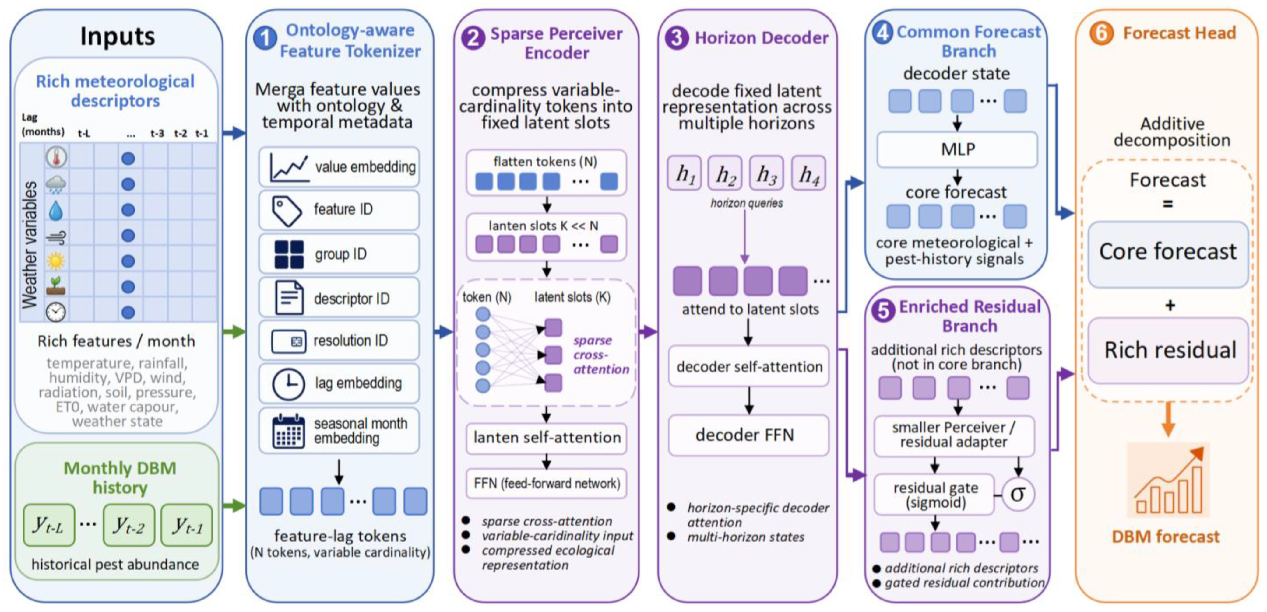
This section defines the forecasting task, descriptor ontology, model architecture, training procedure, and interpretation module. It specifies how the input data are organized, how the large set of lagged weather descriptors is compressed, how forecasts are generated, and how model evidence is summarized. MeteoSCOPE uses monthly DBM abundance and meteorological descriptors from previous months to predict abundance one to four months ahead. Its main design principle is to keep the ecological identity of each descriptor instead of treating the data as an anonymous vector. A schematic overview is shown in Figure 1.

2.1. Forecasting Task and Data Structure

For each site and month, the model receives the previous 12 months of pest and meteorological information and predicts DBM abundance for the next four months. The notation below defines this supervised forecasting task.

Let $t$ denote the current anchor month, $L$ the historical lookback length, and $H$ the number of forecast horizons. In this study, the main forecasting task uses a twelve-month lookback window $L=12$, and four forecast horizons, $H=4$, corresponding to one- to four-month-ahead DBM abundance prediction. For each anchor month $t$, the model receives a lagged rich-feature matrix

$${\mathit{X}}_t={\left[x_{t-\tau ,j}\right]}_{\tau =1,\dots ,L;\hspace{0.25em}j=1,\dots ,F}\in {\mathbb{R}}^{L\times F}.$$

Here, $x_{t-\tau ,j}$ denotes the value of the feature $j$ observed $\tau$ months before the anchor month, and $F$ is the number of meteorological and pest-history features available at each lag. The multi-horizon target vector is defined as:

$${\mathit{y}}_t={\left[y_{t+1},y_{t+2},\dots ,y_{t+H}\right]}^{\mathrm{\top }}\in {\mathbb{R}}^H.$$

In this formulation, $y_{t+H}$ denotes the observed DBM abundance at forecast horizon h, where h = 1, …, H. Because DBM abundance is non-negative and may be highly skewed during outbreak periods, the model is trained on the log-transformed target:

$$z_{t,h}=\mathrm{l}\mathrm{o}\mathrm{g}\left(1+y_{t+h}\right).$$

After inference, forecasts are transformed back to the original abundance scale as

$${\widehat{y}}_{t+h}=\mathrm{e}\mathrm{x}\mathrm{p}\left({\widehat{z}}_{t,h}\right)-1.$$

This formulation defines DBM forecasting as supervised multi-horizon regression from an ecologically annotated feature-lag input to a future abundance vector. The following sections describe how MeteoSCOPE converts each feature-lag cell into an ontology-aware token, compresses the high-dimensional token set through sparse Perceiver-style cross-attention, and decomposes each prediction into a core forecast and enriched residual contribution.

Throughout the manuscript, $t$ denotes the forecast anchor month, $L$ denotes the historical lookback length, $F$ denotes the number of descriptors at each lag, $H$ denotes the number of forecast horizons, $\tau$ indexes historical lag months, and $j$ indexes input descriptors. The matrix $X_t$ denotes the lagged feature table for the anchor month $t$, and $y_{t+h}$ denotes observed DBM abundance at forecast horizon $h.$ In the model architecture, $K$ denotes the number of Perceiver summary slots, while $c_{t,h\prime }{r}_{t,h\prime }$ and ${\widehat{y}}_{t,h}$ denote the core forecast component, enriched residual contribution, and final transformed-scale prediction for the horizon $h$, respectively.

In practical terms, each sample is a structured feature-lag table rather than a flat list of variables. Rows correspond to past months, columns correspond to weather or pest descriptors, and the output contains four future pest-abundance values. This structure is preserved throughout the model so that predictions can later be traced back to ecologically meaningful variables and lag periods.

2.2. Meteorological Descriptor Ontology

The meteorological inputs are designed to describe each month in ecological terms, not only through conventional averages. In addition to levels and totals, the descriptor set includes variability, late-month values, amplitudes, thermal extremes, rainfall intensity, rainy-day rate, dry-spell duration, wind-direction concentration, soil-gradient features, and weather-state frequencies. These descriptors summarize processes that may affect DBM development, survival, host-plant condition, and dispersal.

Each feature is assigned three pieces of metadata that are used by the model and by the interpretation module:

$${\mathcal{M}}_j=\left(g_j,d_j,r_j\right)$$

Here, g_j denotes the ecological group, d_j denotes the descriptor type, and r_j denotes the feature type. Ecological groups include pest history, air temperature, rainfall, humidity and dew point, vapor pressure deficit, wind speed and gust, wind direction, radiation, cloud cover, soil moisture, soil temperature, soil gradient, pressure, boundary-layer height, evapotranspiration, atmospheric water vapor, and weather-state rate. This ontology allows the model to distinguish, for example, temperature extremes from temperature levels, rainfall totals from dry spells, and shallow soil moisture from soil-temperature gradients.

The descriptors are also divided into a core subset and an enriched subset. The core subset contains conventional signals used in pest forecasting, such as temperature, rainfall, relative humidity, wind speed, radiation, shallow soil moisture, and historical pest abundance. The enriched subset contains additional descriptors such as extremes, variability, vapor pressure deficit, cloud cover, deep soil temperature, pressure, evapotranspiration, atmospheric water vapor, and weather-state indicators. This division lets the model estimate a stable core forecast and then measure whether the richer descriptors add or suppress pest risk.

2.3. Model Overview

MeteoSCOPE comprises six components. A tokenizer first converts each feature-lag value into a compact numerical representation that incorporates its ecological metadata, after which the valid tokens are collected into a sequence and missing values are masked. Two sparse Perceiver encoders, one per branch, share an identical architecture but maintain separate parameters and latent slots; each compresses its token sequence into a small set of learned summary slots. Horizon-specific decoders then read from these slots to produce one- to four-month-ahead forecasts. The common branch generates the main forecast from core ecological information, while an enriched residual branch estimates whether the additional descriptors should adjust that forecast upward or downward.

Two design principles guide this architecture. The first is dimensionality control: the model should not require a separate parameter for every lagged descriptor. The second is interpretability: the same structure used for prediction should also support summaries by feature, ecological group, descriptor type, lag period, forecast horizon, and residual contribution.

2.4. Ontology-Aware Feature Tokenizer

The tokenizer is the step that turns raw input values into model-ready tokens. For each anchor month, lag, and feature, the standardized scalar value is combined with learned labels for feature identity, ecological group, descriptor type, feature type, lag position, and seasonal month:

$$u_{t,\tau ,j}=\mathrm{L}\mathrm{N}\left({\varphi }_v\left({\tilde{x}}_{t-\tau ,j}\right)+e_j^{\mathrm{f}\mathrm{e}\mathrm{a}\mathrm{t}}+e_{g_j}^{\mathrm{g}\mathrm{r}\mathrm{p}}+e_{d_j}^{\mathrm{d}\mathrm{e}\mathrm{s}\mathrm{c}}+e_{r_j}^{\mathrm{t}\mathrm{y}\mathrm{p}\mathrm{e}}+e_{\tau }^{\mathrm{l}\mathrm{a}\mathrm{g}}+e_{m_t}^{\mathrm{m}\mathrm{o}\mathrm{n}}\right)$$

In this expression, phi_v(.) is a small value-embedding network; the e-terms are learned embeddings for feature identity, ecological group, descriptor type, feature type, lag position, and seasonal month; and LN denotes layer normalization. The purpose is simple: two values with the same numerical magnitude can still mean different things if they come from different weather processes or different seasons.

Seasonality is included because the same weather condition can have a different biological meaning in different months. For example, a warm month near a seasonal population peak may not play the same role as a warm month in a low-risk period. The anchor month is therefore encoded using a sinusoidal seasonal representation [23]:

$$e_{m_t}^{\mathrm{m}\mathrm{o}\mathrm{n}}=W_m\left[\mathrm{s}\mathrm{i}\mathrm{n}\left(2\pi m_t/12\right),\mathrm{c}\mathrm{o}\mathrm{s}\left(2\pi m_t/12\right)\right]$$

After tokenization, all valid feature-lag tokens are collected into a single sequence:

$$U_t=\left[u_{t,1,1},\dots ,u_{t,1,F},\dots ,u_{t,L,1},\dots ,u_{t,L,F}\right]\in {\mathbb{R}}^{N\times d}, N=L\times F$$

With 12 lag months and 138 descriptors, each sample contains 1656 feature-lag tokens. A binary mask identifies missing or invalid values so that they are not used during attention. This representation keeps the data structured while still allowing the model to process the full rich descriptor set.

2.5. Sparse Perceiver Encoder for Dimensionality Reduction

If every token were compared with every other token, the model would be computationally heavy and prone to overfitting. MeteoSCOPE instead uses a Perceiver-style encoder [29,30]. The encoder introduces a small number of learned summary slots that attend to the input tokens and absorb the most relevant information:

$$Z^{\left(0\right)}=\left[z_1^{\left(0\right)},z_2^{\left(0\right)},\dots ,z_K^{\left(0\right)}\right]\in {\mathbb{R}}^{K\times d}, K\ll N$$

At encoder layer ℓ, the latent slots attend to the input tokens through masked sparse cross-attention:

$$A^{\left(\mathcal{l}\right)}=\mathrm{s}\mathrm{p}\mathrm{a}\mathrm{r}\mathrm{s}\mathrm{e}\mathrm{m}\mathrm{a}\mathrm{x}\left({\displaystyle \frac{\left(Z^{\left(\mathcal{l}-1\right)}{W}_Q\right){\left(U_t{W}_K\right)}^{\mathrm{\top }}}{\sqrt{d}}}+{\Omega }_t\right)$$

Here, the attention mask removes invalid tokens before normalization. Sparsemax [31] is used instead of softmax because it can assign exact zero weights to uninformative tokens. This is useful when many rich weather descriptors are correlated or irrelevant for a particular forecast.

The cross-attended latent representation is computed as:

$${\tilde{Z}}^{\left(\mathcal{l}\right)}=\mathrm{L}\mathrm{N}\left(Z^{\left(\mathcal{l}-1\right)}+A^{\left(\mathcal{l}\right)}\left(U_t{W}_V\right)W_O\right)$$

A latent self-attention block and a feed-forward network are then applied:

$${\overline{Z}}^{\left(\mathcal{l}\right)}=\mathrm{L}\mathrm{N}\left({\tilde{Z}}^{\left(\mathcal{l}\right)}+\mathrm{M}\mathrm{H}\mathrm{A}\left({\tilde{Z}}^{\left(\mathcal{l}\right)}\right)\right)$$

$$Z^{\left(\mathcal{l}\right)}=\mathrm{L}\mathrm{N}\left({\overline{Z}}^{\left(\mathcal{l}\right)}+\mathrm{F}\mathrm{F}\mathrm{N}\left({\overline{Z}}^{\left(\mathcal{l}\right)}\right)\right)$$

The final representation summarizes all pest history and meteorological tokens through a fixed number of summary slots. Its attention cost grows mainly with the number of summary slots and input tokens, rather than with all possible token-token pairs. This makes the architecture suitable for small monthly pest datasets with many lagged descriptors.

2.6. Core Forecast and Enriched Residual Branch

The model separates conventional pest-weather evidence from additional rich descriptors. This is useful because core variables such as pest history, temperature, rainfall, and humidity are expected to provide stable information, whereas enriched descriptors may be redundant or site-specific. The common and enriched branches use two separate Perceiver encoders with branch-specific descriptor subsets and separate parameters, and therefore maintain independent latent slot tensors. The common branch contains historical pest abundance together with the core meteorological variables, so the pest-history-conditioned core forecast is produced there. The enriched branch is not an independent pest-population model: it processes only the additional rich descriptors and produces a gated candidate residual that can adjust, but not replace, the pest-history-conditioned core forecast. Both encoders share the architecture described in Section 2.5. The common branch estimates the core forecast:

$$Z_t^c={\mathrm{P}\mathrm{e}\mathrm{r}\mathrm{c}\mathrm{e}\mathrm{i}\mathrm{v}\mathrm{e}\mathrm{r}}_c\left(U_t^c\right)$$

The enriched branch processes the additional descriptors and produces a candidate correction to the core forecast:

$$Z_t^e={\mathrm{P}\mathrm{e}\mathrm{r}\mathrm{c}\mathrm{e}\mathrm{i}\mathrm{v}\mathrm{e}\mathrm{r}}_e\left(U_t^e\right)$$

For each forecast horizon, a learned query reads the common summary slots. This allows the one-month forecast and the four-month forecast to rely on different parts of the same encoded evidence:

$${\beta }_h^c=\mathrm{s}\mathrm{p}\mathrm{a}\mathrm{r}\mathrm{s}\mathrm{e}\mathrm{m}\mathrm{a}\mathrm{x}\left({\displaystyle \frac{q_h{\left(Z_t^c{W}_{K,h}^c\right)}^{\mathrm{\top }}}{\sqrt{d}}}\right)$$

$$s_{t,h}^c={\displaystyle \sum _{k=1}^K}{\beta }_{h,k}^c{z}_{t,k}^c$$

$$c_{t,h}=f_h^c\left(s_{t,h}^c\right)$$

The enriched branch is decoded in the same spirit, but its output is treated as a correction rather than as a complete forecast:

$${\beta }_h^e=\mathrm{s}\mathrm{p}\mathrm{a}\mathrm{r}\mathrm{s}\mathrm{e}\mathrm{m}\mathrm{a}\mathrm{x}\left({\displaystyle \frac{q_h{\left(Z_t^e{W}_{K,h}^e\right)}^{\mathrm{\top }}}{\sqrt{d}}}\right)$$

$$s_{t,h}^e={\displaystyle \sum _{k=1}^K}{\beta }_{h,k}^e{z}_{t,k}^e$$

$${\delta }_{t,h}=f_h^e\left(s_{t,h}^e\right)$$

A gate controls the size of this correction so that enriched descriptors do not dominate the forecast merely because they are numerous:

$$g_{t,h}=\sigma \left(f_h^g\left(\left[s_{t,h}^c;s_{t,h}^e;q_h\right]\right)\right)$$

$$r_{t,h}=g_{t,h}{\delta }_{t,h}$$

The residual term provides a signed diagnostic. A positive residual means that enriched descriptors increase the predicted pest risk relative to the core forecast; a negative residual means that they reduce it. Thus, the branch is both predictive and interpretable.

2.7. Multi-Horizon Forecasting Head

MeteoSCOPE predicts all four horizons jointly. Separate horizon queries are used because short-term forecasts may rely more on recent pest abundance and recent rainfall, whereas longer-term forecasts may rely more on seasonal temperature patterns, soil moisture, dry spells, vapor pressure deficit, or delayed meteorological effects.

The final prediction on the transformed scale is defined as:

$${\widehat{z}}_{t,h}=b_h+c_{t,h}+r_{t,h}, h=1,2,3,4$$

The predicted DBM abundance on the original scale is obtained by inverse transformation:

$${\widehat{y}}_{t+h}=\mathrm{e}\mathrm{x}\mathrm{p}\left({\widehat{z}}_{t,h}\right)-1$$

This additive form makes the final forecast easier to audit: one part comes from the core ecological forecast, and the other from a gated correction based on richer descriptors.

2.8. Interpretation of Model Evidence

MeteoSCOPE produces explanations by projecting attention back to the annotated feature-lag tokens. Token importance combines two steps: how strongly each summary slot attends to an input token, and how strongly each forecast horizon reads from that summary slot:

$$I_{h,n}={\displaystyle \sum _{k=1}^K}{\beta }_{h,k}{\overline{A}}_{k,n}$$

Because each token corresponds to one feature at one historical lag, token importance can be rearranged into a feature-by-lag map. Summing this map over lags gives feature-level importance:

$$I_{h,j}^{\mathrm{f}\mathrm{e}\mathrm{a}\mathrm{t}}={\displaystyle \sum _{\tau =1}^L}{I}_{h,\tau ,j}$$

Lag-level importance is obtained by summing over features:

$$I_{h,\tau }^{\mathrm{l}\mathrm{a}\mathrm{g}}={\displaystyle \sum _{j=1}^F}{I}_{h,\tau ,j}$$

Group-level and descriptor-level importance are computed by aggregating over the corresponding ontology labels:

$$I_{h,g}^{\mathrm{g}\mathrm{r}\mathrm{p}}={\displaystyle \sum _{\tau =1}^L}\sum _{j:g_j=g}{I}_{h,\tau ,j}$$

$$I_{h,d}^{\mathrm{d}\mathrm{e}\mathrm{s}\mathrm{c}}={\displaystyle \sum _{\tau =1}^L}\sum _{j:d_j=d}{I}_{h,\tau ,j}$$

The importance values are normalized within each forecast horizon using horizon-wise L1 normalization. Specifically, for horizon h, token-level importance is normalized as:

$${\tilde{I}}_{t,h,j,\tau }={\displaystyle \frac{I_{t,h,j,\tau }}{{\displaystyle {\sum }_{j=1}^F}{\displaystyle {\sum }_{\tau =1}^L}{I}_{t,h,j,\tau }+ϵ}}$$

where I_t,h,j,τ is the unnormalized token importance and $\mathsf{ϵ}=10$⁻⁸ prevents division by zero. Feature-, group-, descriptor-, and lag-level scores are then computed by summing Ĩ_t,h,j,τ over the relevant ontology labels or lag indices; therefore, the normalized scores within each horizon sum to one.

Because attention should be interpreted as model evidence rather than causal proof, we also define a feature-set occlusion check. In this check, a group of tokens, such as rainfall, soil moisture, or a specific lag window, is masked, and the forecast is recomputed:

$${\mathrm{\Delta }}_{S,h}={\widehat{z}}_{t,h}\left({\mathit{X}}_t\right)-{\widehat{z}}_{t,h}\left({\mathit{X}}_t^{\left(-S\right)}\right)$$

A positive occlusion contribution indicates that the feature set increases the forecast, whereas a negative contribution indicates that it suppresses the forecast. This perturbation check can be used to test whether attention-based explanations are consistent with changes in predicted abundance.

2.9. Model Training and Regularization

The model is trained on the log-transformed abundance scale. We use the Huber loss because DBM abundance can contain outbreak peaks: the loss is stable for ordinary errors but less sensitive to extreme peaks than squared error alone.

$${\mathcal{L}}_{\mathrm{p}\mathrm{r}\mathrm{e}\mathrm{d}}={\displaystyle \frac{1}{H}}{\displaystyle \sum _{h=1}^H}{\mathrm{H}\mathrm{u}\mathrm{b}\mathrm{e}\mathrm{r}}_{\delta }\left(z_{t,h}-{\widehat{z}}_{t,h}\right)$$

To discourage the enriched residual branch from overfitting noisy or redundant descriptors, the magnitude of the residual correction is penalized:

$${\mathcal{L}}_{\mathrm{r}\mathrm{e}\mathrm{s}}={\displaystyle \frac{1}{H}}{\displaystyle \sum _{h=1}^H}{r}_{t,h}^2$$

The total training objective combines the forecast loss, the residual penalty, and weight decay:

$$\mathcal{L}\left(\Theta \right)={\mathcal{L}}_{\mathrm{p}\mathrm{r}\mathrm{e}\mathrm{d}}+{\lambda }_{\mathrm{r}\mathrm{e}\mathrm{s}}{\mathcal{L}}_{\mathrm{r}\mathrm{e}\mathrm{s}}+{\lambda }_{\mathrm{w}\mathrm{d}}\parallel \Theta {\parallel }_2^2$$

Here, Θ denotes all trainable parameters, λ_res controls the residual penalty, and λ_wd is the weight-decay coefficient. Dropout is applied to token embeddings, summary representations, and feed-forward layers. Feature-group dropout can also be used by randomly masking whole ecological groups during training, which reduces over-reliance on any single meteorological family.

3. Results

This section reports the experimental evaluation of MeteoSCOPE for monthly DBM abundance forecasting at Huiyang and Shantou. Section 3.1 and Section 3.2 describe the experimental setting and evaluation protocol, while Section 3.3 and Section 3.4 present forecasting performance and interpretability results.

3.1. Experimental Settings

We evaluated MeteoSCOPE on monthly DBM abundance records, expressed as DBM larvae per 100 plants, from two stations in Guangdong Province, China: Huiyang (190 observations, March 2005–December 2020) and Shantou (177 observations, April 2006–December 2020). Pest records were provided by the Crop Pest Forecast and Control Center of Guangdong Province, and co-located meteorological observations by the China Meteorological Data Service Center. Each supervised example used a 12-month historical window (L = 12) to predict DBM abundance over the next four months (H = 4), mapping 12 × 138 lagged descriptor values to one-, two-, three-, and four-month-ahead forecasts.

To preserve temporal causality, we partitioned the data chronologically by anchor month into 60/20/20 train, validation, and test sets, fixed at the outset and held constant across all models.

Table 1. Chronological train/validation/test partitions for the Huiyang and Shantou sites.

Partition	Windows	Anchor-Month Span
Huiyang
Train	105–109	September 2005–November 2014
Validation	35–36	October 2014–October 2017
Test	35–36	October 2017–September 2020
Shantou
Train	98–100	October 2006–May 2015
Validation	32–34	February 2015–January 2018
Test	32–34	December 2017–September 2020

reports the resulting partition sizes and anchor-month spans; cutoffs were enforced on the anchor month so that lag features for any test window came strictly from before the held-out period, preventing temporal leakage. Feature scaling and target standardization were fit on the training partition only. Unless otherwise stated, experiments used the rich feature setting (138 descriptors per lag, 1656 feature-lag tokens per sample), with each descriptor annotated by ecological metadata used by the ontology-aware tokenizer and Section 3.4 interpretation analyses: 18 ecological groups and descriptor labels distinguishing summary types (level, variability, extremes, totals, dry-spell duration, late-month values, and weather-state frequencies). Neural models were trained on the transformed target scale (Section 2.1) with metrics computed after inverse transformation, optimized with Adam for up to 300 epochs and early stopping after 20 epochs without validation-MAE improvement. Learning rate, weight decay, batch size, and MeteoSCOPE-specific architectural parameters were tuned with Optuna’s Tree-structured Parzen Estimator on the validation set.

For every site and model, the operating configuration was selected by validation MAE; the test set was used only for final evaluation. Each selected configuration was retrained under ten random seeds (40–49), and the reported results summarize the resulting seed-level distribution.

MeteoSCOPE was compared against ten baselines: Decision Tree, Random Forest, Support Vector Regression, and XGBoost from classical and ensemble learning; and a fully connected ANN, LSTM [32], GRU, Attention-LSTM, Transformer [23], and ALIC [19], an attention-LSTM interaction-CNN model previously developed for explainable DBM forecasting, from deep learning. All baselines were trained and tuned under the same feature scope, chronological split, validation criterion, seed grid, and hyperparameter-search budget as MeteoSCOPE.

All models were implemented in Python 3.12.2. The deep-learning models (MeteoSCOPE, ANN, LSTM, GRU, Attention-LSTM, and Transformer) were built with PyTorch 2.4.1; XGBoost 3.0.2 was used for gradient-boosted trees; scikit-learn 1.6.0 for the Decision Tree, Random Forest, and SVR baselines; Optuna 4.1.0 for hyperparameter optimization; the SHAP package 0.51.0 for KernelSHAP attribution; and SciPy 1.14.1/statsmodels 0.14.4 for the Diebold–Mariano, Wilcoxon signed-rank, and bootstrap analyses. Figures were generated with Matplotlib 3.10.0.

3.2. Evaluation Metrics

Forecasting accuracy was evaluated on the original DBM abundance scale using four regression metrics: mean absolute error (MAE), root mean squared error (RMSE), mean absolute percentage error (MAPE), and coefficient of determination (R²). MAE and RMSE were treated as primary metrics because they are defined for zero-abundance values and are directly interpretable on the abundance scale. MAPE was retained as a secondary relative-error diagnostic because it is sensitive to small non-zero pest counts. R² was used as a complementary measure of explained variation. The horizon-specific metrics were defined as follows:

$$\mathrm{M}\mathrm{A}\mathrm{E}={\displaystyle \frac{1}{N}}{\displaystyle \sum _{i=1}^N}\left|y_i-{\widehat{y}}_i\right|$$

$$\mathrm{R}\mathrm{M}\mathrm{S}\mathrm{E}=\sqrt{{\displaystyle \frac{1}{N}}{\displaystyle \sum _{i=1}^N}{\left(y_i-{\widehat{y}}_i\right)}^2}$$

$$\mathrm{M}\mathrm{A}\mathrm{P}\mathrm{E}={\displaystyle \frac{100}{N^{\prime }}}\sum _{i\in \mathcal{I}}{\displaystyle \frac{\left|y_i-{\widehat{y}}_i\right|}{\left|y_i\right|}}, \mathcal{I}=\{i:y_i\ne 0\}$$

$$R^2=1-{\displaystyle \frac{{\displaystyle {\sum }_{i=1}^N}{\left(y_i-{\widehat{y}}_i\right)}^2}{{\displaystyle {\sum }_{i=1}^N}{\left(y_i-\bar{y}\right)}^2}}$$

where I is the set of non-zero ground-truth observations and N′ = |I|. MAE, RMSE, and MAPE are lower-is-better; R² is higher-is-better and is unbounded below. To avoid undefined ratios, MAPE is computed only over samples with non-zero DBM abundance counts.

For each site, model, and seed, metrics were first computed separately at each forecast horizon. The headline value for a given seed was then obtained by averaging over the four horizons:

$${\overline{m}}_s={\displaystyle \frac{1}{H}}{\displaystyle \sum _{h=1}^H}{m}_{s,h}.$$

The final reported value was the mean across the ten seeds:

$$\overline{m}={\displaystyle \frac{1}{S}}{\displaystyle \sum _{s=1}^S}{\overline{m}}_s,$$

The accompanying uncertainty term is the standard deviation across the ten seed-level horizon-averaged values. This aggregation reports performance over the full one- to four-month forecasting block while preserving seed-level variation for paired statistical analysis.

Pairwise statistical comparisons were conducted between MeteoSCOPE and each baseline separately for each site and metric. For error metrics, the effect size was baseline minus MeteoSCOPE; for R², it was MeteoSCOPE minus baseline. Thus, positive values always indicate an advantage for MeteoSCOPE.

Three complementary statistical procedures were used. First, horizon-specific Diebold-Mariano tests were applied to ordered test-window loss differentials. For a baseline model b, the loss differential at horizon h was defined as:

$$d_{i,h}^{\left(b\right)}=\mathcal{l}\left(y_{i,h},{\widehat{y}}_{i,h}^{\left(b\right)}\right)-\mathcal{l}\left(y_{i,h},{\widehat{y}}_{i,h}^{\left(\mathrm{MeteoSCOPE}\right)}\right).$$

The loss function was absolute error for MAE, squared error for RMSE and R², and absolute percentage error for MAPE after excluding zero-abundance observations. The Diebold-Mariano statistic used the Harvey-Leybourne-Newbold small-sample correction and a Newey–West heteroskedasticity- and autocorrelation-consistent variance estimator with Bartlett kernel bandwidth h − 1, reflecting serial dependence induced by overlapping multi-step forecast windows. The directional alternative was that MeteoSCOPE had a lower expected loss than the baseline. Second, seed-level robustness was assessed with Wilcoxon signed-rank tests on paired horizon-averaged metric values across ten random seeds. Third, effect-size uncertainty was quantified with 95% percentile bootstrap confidence intervals computed from 10,000 paired seed-level resamples.

Multiple-testing correction was applied within each site–metric family. Aggregated pairwise comparisons against the ten baselines were corrected using the Holm–Bonferroni procedure. Horizon-specific Diebold–Mariano comparisons, covering ten baselines across four horizons, were corrected using the Benjamini–Hochberg false-discovery-rate procedure. Forecasting performance is therefore interpreted using three pieces of evidence jointly: the magnitude of the effect size, the bootstrap confidence interval, and the corrected paired-test results.

3.3. Overall Forecasting Performance Against Benchmark Models

Table 2. Multi-horizon DBM forecasting performance of MeteoSCOPE and benchmark models under the rich feature setting.

Model	MAE	RMSE	MAPE (%)	R2
Huiyang
Decision Tree	51.46 ± 1.42 ***	85.60 ± 1.38 ***	291.8 ± 47.0	0.121 ± 0.032 ***
Random Forest	40.95 ± 0.29 *	71.38 ± 0.38	255.1 ± 6.0 **	0.410 ± 0.006
SVR	49.36 ± 0.00 ***	94.46 ± 0.00 ***	208.1 ± 0.0	−0.033 ± 0.000 ***
XGBoost	43.24 ± 0.00 *	69.75 ± 0.00	360.8 ± 0.0 ***	0.434 ± 0.000
ANN	42.69 ± 1.92 *	72.84 ± 2.75	160.2 ± 17.8	0.383 ± 0.047
LSTM	41.05 ± 2.91 *	71.35 ± 3.99	185.6 ± 38.0	0.408 ± 0.068
GRU	52.38 ± 4.25 ***	72.60 ± 3.46	543.4 ± 110.4 ***	0.378 ± 0.063
Attn-LSTM	47.33 ± 4.97 **	79.49 ± 8.17 **	197.4 ± 72.8	0.251 ± 0.151 **
Transformer	50.56 ± 4.37 ***	75.59 ± 4.37 ***	473.3 ± 109.5 ***	0.333 ± 0.077 ***
ALIC	41.76 ± 2.11 *	70.18 ± 2.82	201.5 ± 33.9	0.427 ± 0.046
MeteoSCOPE (ours)	38.86 ± 3.85	69.14 ± 4.98	206.9 ± 79.7	0.442 ± 0.078
Shantou
Decision Tree	37.20 ± 0.69 **	47.18 ± 0.92 **	50.4 ± 0.7 ***	0.114 ± 0.035 **
Random Forest	32.32 ± 0.41 *	39.19 ± 0.44 *	46.7 ± 0.5 ***	0.386 ± 0.014 *
SVR	52.31 ± 0.00 ***	58.74 ± 0.00 ***	80.2 ± 0.0 ***	−0.328 ± 0.000 ***
XGBoost	33.89 ± 0.00 **	40.45 ± 0.00 *	45.7 ± 0.0 ***	0.343 ± 0.000 *
ANN	46.20 ± 4.09 ***	52.56 ± 4.54 ***	68.4 ± 7.2 ***	−0.084 ± 0.205 ***
LSTM	42.60 ± 5.24 ***	51.17 ± 5.54 ***	56.3 ± 7.4 ***	−0.018 ± 0.222 ***
GRU	33.14 ± 4.35 **	40.52 ± 5.09 *	46.0 ± 6.3 ***	0.342 ± 0.172 *
Attn-LSTM	41.93 ± 6.64 ***	52.41 ± 8.40 ***	62.7 ± 11.1 ***	−0.111 ± 0.334 ***
Transformer	32.69 ± 3.40 **	40.71 ± 3.67 *	47.2 ± 6.4 ***	0.339 ± 0.120 *
ALIC	35.72 ± 5.70 ***	44.32 ± 6.41 ***	48.8 ± 8.3 ***	0.226 ± 0.223 ***
MeteoSCOPE (ours)	28.54 ± 2.77	35.63 ± 3.33	35.7 ± 5.3	0.473 ± 0.104

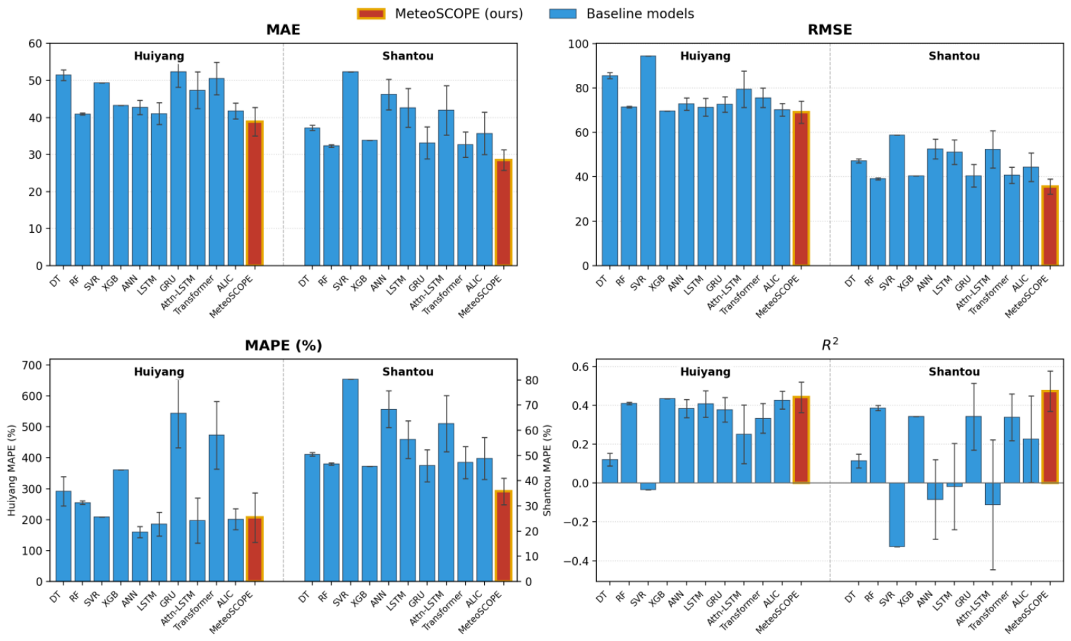
Notes: Values are mean ± standard deviation across ten random seeds after averaging over four forecast horizons. Bold indicates the best model within each site-metric block, and underlining indicates the second-best model. Superscripts indicate Holm-corrected one-sided Diebold-Mariano significance against MeteoSCOPE (* p < 0.05, ** p < 0.01, *** p < 0.001).

and Figure 2 summarize the four-horizon forecasting performance of MeteoSCOPE and ten benchmark models under the rich-feature, 12-month lookback setting. The baselines span classical regressors (Decision Tree, Random Forest, SVR, and XGBoost), generic neural sequence models (ANN, LSTM, GRU, Attention-LSTM, and Transformer), and ALIC, the closest pest-specific comparator, which combines feature attention, recurrent temporal encoding, and an interaction-CNN module for meteorological and historical pest inputs [19].

MeteoSCOPE provides the best overall error profile across the two monitoring sites, although the magnitude and stability of the gains are site-dependent. On Huiyang, it achieves the lowest MAE and RMSE. The MAE decreases from 40.95 for the strongest baseline, Random Forest, to 38.86, a 5.1% reduction, while RMSE decreases to 69.14 relative to 69.75 for XGBoost and 70.18 for ALIC. These gains indicate a lower absolute forecasting error, but they are modest in variance-sensitive terms, and MeteoSCOPE is not the leading model under MAPE.

The Shantou results are more pronounced. MeteoSCOPE is the best-performing model on all four metrics, reducing MAE from 32.32 for Random Forest to 28.54 (an 11.7% reduction), RMSE from 39.19 to 35.63, and MAPE from 45.7% for XGBoost to 35.7%. It also increases R² from 0.386 for Random Forest to 0.473. This broader improvement suggests that, at Shantou, the ontology-aware sparse Perceiver is particularly effective at combining recent pest history with site-specific meteorological evidence.

The benchmark comparison further shows that competitive performance is distributed across model families rather than concentrated in a single alternative. Random Forest is the strongest non-neural comparator for MAE, XGBoost remains competitive for Huiyang RMSE and R², and GRU and Transformer are competitive on selected Shantou metrics. ALIC remains an informative pest-specific baseline, but its compact interaction design does not match MeteoSCOPE when the input is expanded into a high-dimensional set of structured feature-lag tokens. This pattern supports the central premise of the proposed architecture: rich meteorological descriptors require a controlled compression mechanism that preserves ecological structure while avoiding an unconstrained dense representation of all lagged variables.

Because DBM abundance is sparse and can approach zero in some months, MAPE is more volatile than MAE or RMSE and should not be treated as the primary performance criterion. We therefore interpret MAE and RMSE as the main accuracy measures and retain MAPE as a scale-normalized diagnostic. This distinction is especially important for Huiyang, where MeteoSCOPE improves both primary absolute-error metrics but does not minimize percentage error.

From a high-dimensional data-analysis perspective, these results indicate that the performance gain is not produced merely by increasing the number of meteorological inputs. The same rich feature space is available to all models, yet MeteoSCOPE is better able to organize this information through feature-lag tokenization, latent-bottleneck compression, and horizon-specific decoding. The comparison therefore supports the methodological claim that high-dimensional agricultural monitoring data require architectures that preserve ecological structure while controlling statistical complexity.

3.4. Interpretability of MeteoSCOPE

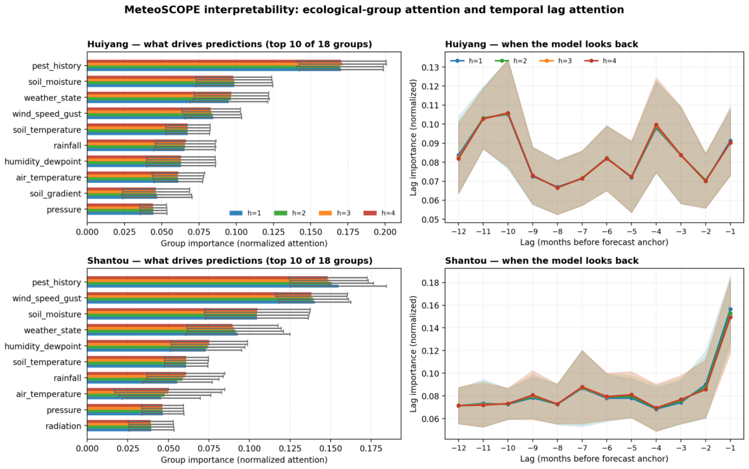
MeteoSCOPE’s interpretation module was designed as a multidimensional decomposition of model evidence. Because each input token corresponds to a specific feature-lag cell and carries metadata for feature identity, ecological group, descriptor type, feature category, lag position, and seasonal month, attention weights can be projected back onto agronomically meaningful axes (

Table 3. Multidimensional interpretation summary for MeteoSCOPE.

Site	Dominant Ecological Groups	Dominant Lags
Huiyang	Pest history; soil moisture; weather state; wind speed/gust; soil temperature	−10, −11, −4
Shantou	Pest history; wind speed/gust; soil moisture; weather state; humidity/dew point	−1, −7, −2

Notes: Dominant ecological groups and dominant lags are normalized attention averages across test windows, forecast horizons, and ten random seeds.

). The resulting explanations summarize model evidence across ecological groups, descriptor families, temporal lags, forecast horizons, and branch-level residual contributions (Figure 3). This converts the latent routing behavior of the sparse Perceiver into auditable summaries that can be inspected by agronomists and pest-management specialists.

Interpretations were averaged across held-out test windows and ten random seeds. The main text focuses on three explanation levels that are directly auditable and biologically interpretable: ecological-group attribution, temporal-lag attribution, and horizon-level stability. Descriptor-level and individual token-level tensors are generated by the same attention map and are vailable from the authors upon reasonable request when feature-by-feature agronomic inspection is required.

3.4.1. Ecological-Group Attribution

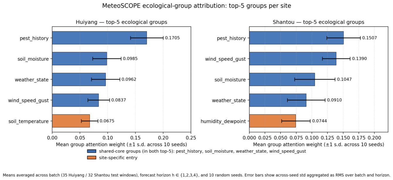
Figure 4 summarizes ecological-group attribution across sites. Pest history is the dominant group in both cases, accounting for 17.0% of normalized group attention on Huiyang and 15.1% on Shantou. This result confirms that DBM forecasting is strongly autoregressive: recent and historical abundance provides the most informative evidence for future population levels.

The secondary ecological signals are site-specific. At Huiyang, the leading non-pest groups are soil moisture, weather-state indicators, wind speed/gust, and soil temperature, suggesting a regime shaped by pest persistence, soil-water status, and seasonal thermal context. At Shantou, wind speed/gust rises to second place, followed by soil moisture, weather-state indicators, and humidity/dew point. This pattern is consistent with a coastal setting in which maritime moisture and wind conditions may influence adult movement, survival, and host-plant microclimate.

These contrasts illustrate why ontology-level attribution is preferable to a flat list of covariates. A flat ranking would identify individual variables, but it would not reveal that the model evidence suggests different site-specific regimes: a soil-temperature and seasonal-memory regime at Huiyang, and a wind-humidity, short-range regime at Shantou.

3.4.2. Temporal-Lag Attribution

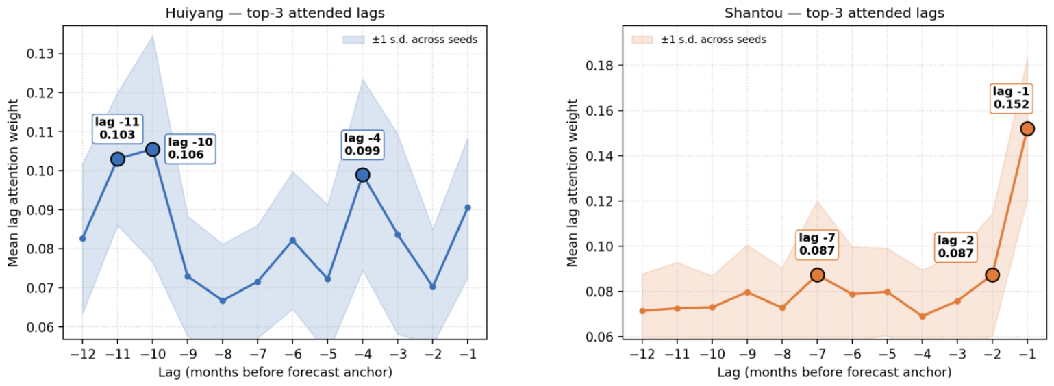
Figure 5 shows the corresponding temporal-lag attribution. Huiyang places most attention on longer lags, especially lag −10 and lag −11, with an additional contribution from lag −4. This pattern suggests that the model uses year-on-year seasonal memory, inferring current pest risk partly from conditions close to the same season in the previous annual cycle.

Shantou exhibits a shorter memory structure. The largest lag attribution occurs at lag −1, which receives approximately 15.2% of the lag-attention budget, followed by secondary peaks near lag −7 and lag −2. Forecasting at this site therefore resembles structured nowcasting: recent pest and meteorological conditions dominate, while a weaker mid-range seasonal signal remains detectable.

Together, the group and lag attributions show that MeteoSCOPE does not impose a single universal explanation across sites. Instead, it learns site-specific ecological evidence patterns while retaining a common architecture, feature ontology, and attribution procedure.

3.4.3. Horizon-Level Behavior

The horizon-level overlays show that the dominant groups and lag peaks remain largely stable from one to four months ahead. On Huiyang, pest history, soil moisture, and weather-state indicators remain the principal groups across horizons; on Shantou, pest history, wind speed/gust, and soil moisture remain dominant. The lag-attention profiles also shift only modestly across forecast horizons.

This stability suggests that MeteoSCOPE learns a shared site-specific ecological representation and then projects it through horizon-specific output queries, rather than learning four unrelated forecasting mechanisms. For decision support, this is useful: pest managers can audit one dominant ecological regime per site while still receiving separate forecasts for each planning horizon.

3.4.4. Validation of Attention Attributions by Independent Methods

Although the attention-derived feature importances are biologically plausible, attention weights do not inherently guarantee causal significance or robust output impact. To rigorously test whether the identified attention profiles reflect genuine model reliance, we conducted two independent post hoc perturbation tests, namely Feature-Set Occlusion and Group-Level KernelSHAP, applied to the ten multi-seed checkpoints without retraining.

To systematically implement these empirical checks, we designed two distinct mapping mechanisms. For the feature-set occlusion protocol, all input tokens belonging to a target ecological group were sequentially masked using the training-time mask Ω_t (forcing attention weights to zero). The resulting signed output divergence, Δ_t,g,h = ẑ_t,h(X_t) − ẑ_t,h(X_t∖S_g), was computed across all test windows, random seeds, and forecast horizons. For the group-level KernelSHAP protocol, each of the 18 ecological groups was treated as a binary super-feature toggled via the same Ω_t mask. To manage computational complexity while preserving validation fidelity, Shapley values were derived using 100 sampled coalitions per point against a background of 50 k-means clusters of training set means, evaluated specifically at the first forecast horizon (h = 1). For both validation methods, the importance of each group was aggregated as the mean absolute contribution across all evaluation windows and seeds, with rank consistency quantified using Spearman rank correlation (ρ) and top-k intersection counts.

The statistical alignments summarized in

Table 4. (a) Consistency and rank agreement between attention-based group attributions, feature-set occlusion, and KernelSHAP. (b) Top-3 ecological-group rankings at horizon h = 1 across verification methods.

(a)
Site		Horizon	Method	Spearman ρ		p-Value	Top-3 Overlap		Top-5 Overlap
Huiyang		h = 1	Occlusion	0.822		2.8 × 10−5	2/3		2/5
			KernelSHAP	0.713		8.9 × 10−4	2/3		2/5
		h = 2	Occlusion	0.814		3.9 × 10−5	2/3		2/5
		h = 3	Occlusion	0.785		1.1 × 10−4	2/3		2/5
		h = 4	Occlusion	0.827		2.3 × 10−5	2/3		2/5
Shantou		h = 1	Occlusion	0.868		3.1 × 10−6	2/3		4/5
			KernelSHAP	0.670		2.4 × 10−3	2/3		4/5
		h = 2	Occlusion	0.872		2.4 × 10−6	2/3		3/5
		h = 3	Occlusion	0.903		2.9 × 10−7	2/3		4/5
		h = 4	Occlusion	0.864		3.9 × 10−6	2/3		4/5
(b)
Site	Attention Top-3		Occlusion Top-3		SHAP Top-3			Agreed Across All Three
Huiyang	pest_history, soil_moisture, weather_state		pest_history, weather_state, air_temperature		pest_history, weather_state, air_temperature			pest_history, weather_state
Shantou	pest_history, wind_speed_gust, soil_moisture		pest_history, wind_speed_gust, weather_state		wind_speed_gust, pest_history, soil_gradient			pest_history, wind_speed_gust

a,b confirm that the baseline attention attributions are highly robust and heavily corroborated by independent output-perturbation tests. Specifically, the Spearman rank correlation between attention intensity and occlusion-driven importance is uniformly strong across all four forecast horizons, with ρ ranging from 0.79 to 0.83 at Huiyang and from 0.86 to 0.90 at Shantou (p < 0.0001). Furthermore, the KernelSHAP evaluations at h = 1 strongly resonate with these distributions, yielding significant correlations of ρ = 0.713 (p = 0.00089) at Huiyang and ρ = 0.670 (p = 0.0024) at Shantou. This cross-method intersection reveals that the primary pest history component is consistently identified as the leading predictive driver across all three distinct evaluation frameworks at Huiyang. For the coastal Shantou regime, while the baseline attention and occlusion frameworks rank pest history first, KernelSHAP elevates wind speed and gust to the top tier, with pest history as a close second. Despite minor internal rank variations among secondary meteorological factors, the collective convergence among these complementary counterfactual approaches—ranging from leave-one-out masking to coalition-weighted Shapley expectations—substantiates the structural interpretations established in Section 3.4.1. This multi-angle verification verifies that MeteoSCOPE captures authentic, site-specific environmental signatures rather than localized attention artifacts, bounding the explanatory framework within an auditable, scientifically sound scope.

3.5. Ablation Study

To quantify the individual contribution of each architectural component within MeteoSCOPE, we conducted a controlled ablation study consisting of seven variants. The detailed configurations of these variants are formalized in

Table 5. Configuration of the seven ablation variants.

Variant	Architectural Change
(a) Full MeteoSCOPE	Reference. All architectural components enabled as in Section 2.4, Section 2.5, Section 2.6 and Section 2.7.
(b) Ontology metadata embeddings	Feature-identity, ecological-group, descriptor-type, feature-type and seasonal-month embeddings are removed; the tokenizer outputs the value-MLP projection ϕ_v plus the lag embedding only.
(c) Sparsemax → softmax	Sparsemax replaced by softmax in the cross-attention of both Perceiver encoders.
(d) Dual-branch enriched residual	Enriched encoder, residual decoder, gating MLP and residual penalty λ_res removed; the prediction is the common-branch output only.
(e) Horizon-specific queries	Four horizon-specific queries q_h replaced by a single shared query broadcast over the H horizons.
(f) Reduced K = 4 in both encoders	Latent slot count fixed to K = 4 (defaults: K = 26 common, K = 16 enriched).
(g) Core (compact) feature input	Input restricted to the 10 conventional monthly meteorological signals plus the one-month-lagged pest history (132 tokens at L = 12).

. All variants were systematically trained and evaluated under the identical chronological dataset split (60/20/20), feature settings, and multi-seed hyperparameter optimization workflow described in Section 3.1 and Section 3.3. All performance metrics were calculated on the original insect abundance scale, horizon-averaged per seed, and subsequently aggregated across ten random seeds.

Table 6. Multi-horizon DBM forecasting performance under each ablation variant. Values represent the mean ± standard deviation across ten random seeds after horizon averaging. Significance stars (* p_Holm < 0.05) indicate pairs derived from a two-sided Wilcoxon signed-rank test against the full baseline (a) within each (site × metric) family.

Variant	Huiyang MAE	Huiyang RMSE	Huiyang MAPE	Huiyang R2	Shantou MAE	Shantou RMSE	Shantou MAPE	Shantou R2
(a) Full	41.76 ± 6.20	69.33 ± 4.11	297.9	0.438	30.15 ± 3.94	38.16 ± 4.73	40.88	0.406
(b) Ontology	42.76 ± 1.76	76.20 ± 3.01	211.9	0.325	46.29 *	53.01 *	67.69 *	−0.119 *
(c) Sparsemax	39.14 ± 3.07	67.75 ± 4.11	256.3	0.462	43.66 *	51.32 *	63.14 *	−0.056 *
(d) Dual branch	40.02 ± 1.96	69.21 ± 1.89	205.9	0.444	38.07	45.63	51.83	0.138
(e) Horizon queries	39.91 ± 2.16	69.30 ± 4.37	195.6	0.439	35.48 *	44.10	46.26	0.225
(f) K = 4	41.88 ± 3.32	69.86 ± 5.44	262.0	0.429	36.51	43.80	51.47	0.209
(g) Core feature input	40.69 ± 3.27	70.20 ± 4.79	216.9	0.423	33.86	42.14	46.00	0.293

details the horizon-averaged forecasting performance for each ablation variant across both experimental sites. Statistical significance was evaluated relative to the full MeteoSCOPE baseline, with key structural variants demonstrating distinct site-specific impacts.

For the Shantou site, four of the six ablations severely degraded predictive accuracy. Strikingly, removing the ontology metadata embeddings (variant b) increased the MAE by 53.5% and collapsed the R² from 0.406 to −0.119 (p_Holm = 0.012). A comparable degradation occurred when replacing the sparsemax attention with standard softmax (variant c; MAE +44.8%, p_Holm = 0.020), underscoring the necessity of sparse attention in filtering meteorological noise. The shared-query decoder (variant e) also exhibited significant performance loss (MAE +17.7%, p_Holm = 0.039). While the removal of the dual-branch structure (variant d) displayed a directional performance drop (MAE +26.3%), it did not achieve strict statistical significance (p_Holm = 0.082) under the 10-seed constraint. In contrast, no architectural ablation reached statistical significance at the Huiyang site. The most pronounced change was observed in variant (b) with a marginal 2.4% increase in MAE, which remains well within the baseline seed-to-seed variance (±6.20). This minimal sensitivity conforms to the insights from Section 3.3 and Section 3.4: because Huiyang’s diamondback moth dynamics are predominantly autoregressive (dominated by historical pest density), variations in the meteorological processing components yield limited leverage over the final forecast. In summary, ontology-aware tokenization and sparse cross-attention represent the primary drivers of MeteoSCOPE’s forecasting proficiency in scenarios with complex environmental backdrops (Shantou), whereas horizon-specific decoding acts as a meaningful secondary contributor. Regarding experimental boundaries, we note that the seasonal-month embedding was unactivated across all runs due to data-adapter constraints (meaning variant b isolates the core ontology effect), and variant (e) introduces a minor 192-parameter reduction. However, these boundary conditions do not materially alter the structural insights gained from this ablation.

3.6. Learning-Curve Analysis

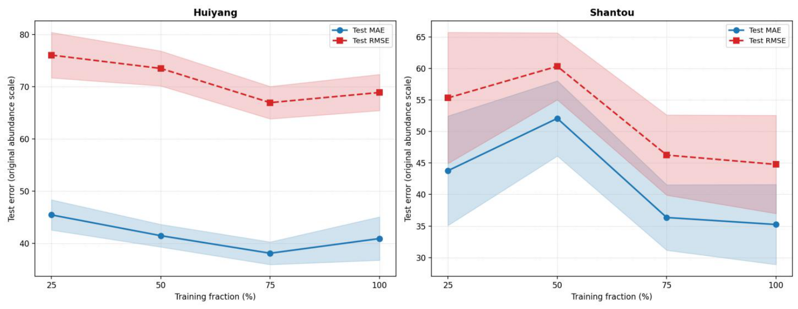
To investigate whether the 1656-token MeteoSCOPE configuration overfits the available small-sample regime, we evaluated predictive behavior across a gradient of training-data fractions, setting f ∈ {0.25, 0.50, 0.75, 1.00}. For each fraction, models were trained exclusively on the chronologically earliest f-proportion of the training partition, while validation and test sets remained unaltered. Feature standardization was refit strictly on each truncated subset. To ensure consistency with the baseline, an independent Optuna TPE search (n_trials = 30) followed by a ten-seed retraining workflow was executed for each (site, fraction) configuration. The resulting test metrics for both locations are consolidated in

Table 7. (a). Multi-site DBM forecasting performance across different training-data fractions. (b). Per-site 0.75 → 1.00 slope summary. A ratio below one indicates the change is within the seed-level noise envelope at f = 1.00.

(a)
	Training Fraction	MAE	RMSE		MAPE		R2
Huiyang	f = 0.25	45.47 ± 2.90	76.06 ± 4.35		271.3 ± 83.6		0.322 ± 0.076
	f = 0.50	41.49 ± 2.16	73.50 ± 3.34		173.3 ± 29.4		0.369 ± 0.060
	f = 0.75	38.13 ± 2.17	66.95 ± 3.10		198.1 ± 50.8		0.477 ± 0.049
	f = 1.00	40.94 ± 4.15	68.90 ± 3.46		281.3 ± 117.8		0.448 ± 0.056
Shantou	f = 0.25	43.77 ± 8.68	55.31 ± 10.40		64.25 ± 14.58		−0.288 ± 0.515
	f = 0.50	52.07 ± 5.97	60.33 ± 5.31		76.42 ± 11.98		−0.452 ± 0.239
	f = 0.75	36.35 ± 5.19	46.26 ± 6.37		48.25 ± 7.48		0.122 ± 0.232
	f = 1.00	35.24 ± 6.35	44.77 ± 7.79		45.14 ± 7.06		0.175 ± 0.296
(b)
Site	MAE @ 0.75	MAE @ 1.00	Δ MAE	Combined σ		|Δ|/σ		Verdict
Huiyang	38.13	40.94	+2.81	3.31		0.85		Saturating (within seed noise)
Shantou	36.35	35.24	−1.11	5.80		0.19		Saturating (within seed noise)

.

As illustrated in Table 7a and Figure 6, the two experimental sites exhibit distinct data-scaling trajectories. At the Huiyang site, the test MAE decreases monotonically from 45.47 (f = 0.25) to 38.13 (f = 0.75), before exhibiting a minor statistical bounce to 40.94 at f = 1.00. To determine whether this late-stage variation constitutes genuine overfitting or baseline variance, we established a noise-aware slope summary in Table 7b, which quantifies the ratio of performance changes relative to seed-level noise.

As detailed in

Table 8. Cross-site transfer results. Mean ± standard deviation across ten random seeds after horizon-averaging.

Protocol	MAE	RMSE	MAPE	R2
Huiyang within-site (reference)	41.76 ± 6.20	69.33 ± 4.11	297.9	0.438 ± 0.068
Shantou within-site (reference)	30.15 ± 3.94	38.16 ± 4.73	40.88	0.406 ± 0.163
Huiyang to Shantou (transfer)	47.05 ± 5.02	57.49 ± 4.52	48.83	−0.283 ± 0.201
Shantou to Huiyang (transfer)	87.87 ± 9.36	98.82 ± 8.16	1618.6	−0.157 ± 0.195

, the transition from f = 0.75 to f = 1.00 at Huiyang (MAE +2.81) translates to merely 0.85 of the combined seed standard deviation (σ = 3.31). This indicates that the learning curve flattens within the inherent seed noise envelope rather than signaling the onset of overfitting. Conversely, the Shantou site displays a less monotonic but sustained downward trajectory, with the MAE dropping from 43.77 to 35.24; as shown in Table 8, the final training fraction increment from 0.75 to 1.00 (MAE −1.11) similarly falls well within the seed noise threshold (a ratio of 0.19).

Crucially, neither site exhibits the distinctive inflection points in error metrics that typically characterize overparameterized overfitting. Instead, the scaling profiles indicate that generalization error in this sample range is primarily bounded by representational capacity and label noise rather than training-set volume. Additionally, the Huiyang MAPE trajectory (fluctuating from 271% to 281% despite a stable MAE profile in Table 7a) underscores our rationale in Section 3.2 for treating MAPE strictly as a secondary diagnostic due to its mathematical sensitivity to near-zero abundance baselines. While these ten-seed empirical trajectories provide a discretized view of saturation, they sufficiently demonstrate that the current model capacity is well-calibrated to the historical data volume available at both stations.

3.7. Cross-Site Zero-Shot Transferability

Section 3.3 reports per-site accuracy under site-specific training; a complementary question is how site-specific the learned representation is. We evaluate strict zero-shot cross-site transfer: no target-site data—labels, inputs, or statistics—is exposed to the model or its scalers during training or hyperparameter selection.

Two complementary directional protocols were executed: Protocol A (Huiyang to Shantou) was trained and hyperparameter-tuned via Optuna strictly on the Huiyang partitions, with all feature and target scalers frozen on Huiyang training statistics. The optimal configuration was retrained across ten seeds (40–49) on combined Huiyang training and validation sets, and subsequently evaluated on the raw Shantou test partition without any parameter or scaler recalibration. Protocol B (Shantou to Huiyang) represents the exact spatial mirror of Protocol A. Within-site reference baselines were derived from the full MeteoSCOPE execution detailed in Section 3.5 to guarantee identical code paths, random seeds, and aggregation protocols.

The absolute performance metrics resulting from these cross-site transfers are presented in Table 8, while the localized forecasting gaps relative to within-site references are compiled in

Table 9. Per-transfer gap relative to the target’s within-site reference.

Transfer Protocol	Within MAE	Transfer MAE	Δ MAE	Δ %	Within RMSE	Transfer RMSE	Δ RMSE	Δ %
Huiyang  to Shantou (transfer)	30.15	47.05	+16.90	+56.1	38.16	57.49	+19.32	+50.6
Shantou to Huiyang (transfer)	41.76	87.87	+46.11	+110.4	69.33	98.82	+29.49	+42.5

.

In the Huiyang to Shantou transfer, the model suffers an MAE inflation gap of +16.90 (+56.1%) and an RMSE gap of +19.32 (+50.6%), collapsing the R² from a baseline of 0.406 to −0.283. This degradation is exacerbated in the Shantou to Huiyang direction, where the MAE gap expands by +46.11 (+110.4%), and the R² drops to −0.157. In both instances, cross-site zero-shot transfer reduces the model from an operationally viable forecaster to one that underperforms a simple historical constant mean (R² < 0).

Interestingly, a structural asymmetry is observable in the Shantou to Huiyang transfer in Table 9, characterized by a massive MAE inflation alongside a relatively tempered RMSE degradation. This specific divergence indicates that the transferred model fails primarily due to systemic miscalibration during typical low-to-moderate abundance months, rather than an inability to capture extreme population peaks. This finding strongly aligns with the attention attributions in Section 3.4, which demonstrated that the model relies on distinct secondary ecological groups unique to each geographic site. Collectively, the zero-shot performance gap demonstrates that MeteoSCOPE successfully captures highly localized, site-specific ecological drivers of diamondback moth dynamics. Consequently, while these results bound the architecture’s direct zero-shot transferability, they highlight the necessity of localized fine-tuning or joint multi-site training strategies, which represent promising avenues for future regional-scale-up operational deployments.

4. Discussion

This study establishes MeteoSCOPE as a high-capacity, structured retrospective forecasting framework for diamondback moth (DBM, P. xylostella) abundance. While complementary to real-time, field-level monitoring sensors that handle immediate warning, this multi-horizon architecture operates as a long-term strategic vehicle. Under a rigorous chronological evaluation pipeline—including training-only scaling, validation-based selection, and temporally held-out testing—the architecture eliminates risk of temporal leakage and consistently delivers accurate multi-horizon predictions. Structurally, MeteoSCOPE extends traditional black-box forecasting by offering a long-term strategic decision-support window up to four months. This predictive capability enables regional plant protection departments to confidently anticipate seasonal infestation baselines during early sowing phases, optimize the proactive management of biological controls, and adapt local crop-rotation strategies well in advance.

The empirical validation further highlights that MeteoSCOPE maintains a highly robust global performance profile while successfully managing site-specific data characteristics. At Shantou, the architecture achieves a broad advantage across all evaluated metrics, while at Huiyang, it reliably maintains the lowest absolute error (MAE and RMSE). This site-dependent alignment is particularly valuable for low-count pest abundance regimes, where absolute-error optimization offers greater operational reliability than unstable percentage diagnostics like MAPE. Ultimately, MeteoSCOPE’s primary contribution lies in this unique combination of competitive forecasting precision with structured, ontology-aware explanations that can be directly audited by pest-management specialists.

The interpretation results are most useful when read against Guangdong’s heterogeneous vegetable-production landscapes. DBM dynamics are shaped not only by temperature, rainfall, and humidity, but also by host continuity, cropping pattern, local management history, insecticide pressure, natural enemies, microclimate, and dispersal. Previous studies on DBM in Guangdong and China emphasize that climate, migration, natural enemies, cropping systems, and management practices jointly affect population dynamics in Brassica production systems [33,34,35]. Against this background, MeteoSCOPE’s per-token and per-lag explanations provide an agronomic audit trail: they indicate whether a forecast is mainly supported by local pest-history accumulation, delayed field-environmental memory, or recent meteorological evidence consistent with dispersal. These explanations should be interpreted as model evidence rather than causal proof.

At the inland Huiyang, the dominant pest-history signal and the strong attention to lags −10 and −11 suggest a long-memory, crop-calendar-linked regime. This pattern is consistent with an inland or peri-inland vegetable-production setting in which recurrent Brassica cultivation, seasonal host availability, and local control history preserve information from the previous annual cycle. Historical pest abundance may therefore summarize local population carryover, host continuity, residual infestation pressure, and previous management outcomes. The secondary attention to soil moisture, weather-state indicators, and soil temperature suggests that the model uses field microclimate and host-environment proxies to adjust this pest-history signal. Because DBM pupation generally occurs in loose silk cocoons on host-plant surfaces rather than in soil [36], soil moisture and soil temperature should be interpreted conservatively as proxies for canopy and near-surface microclimate, host-plant water status, and habitat persistence, rather than as direct evidence for soil-stage survival.

At the coastal Shantou, the attribution pattern is different. The leading temporal lag is −1 month, and wind speed/gust is consistently among the strongest non-pest ecological groups. This supports a coastal, short-memory, wind-associated regime. Shantou is located in eastern coastal Guangdong, where maritime humidity, sea–land airflow, and gust events can rapidly alter field microclimate and may also influence adult movement, landing, and local colonization. This interpretation is consistent with DBM’s documented capacity for wind-assisted movement and long-distance migration, including evidence that monsoon systems can facilitate DBM movement within China [37]. Thus, Shantou forecasts appear to rely less on annual local carryover alone and more on recent pest abundance together with wind and humidity signals that may reflect short-term immigration, settlement, and population growth.

This site contrast has practical value for decision support. A black-box forecast can warn that DBM abundance may increase, but it cannot indicate whether the warning is mainly supported by local pest-source accumulation or by recent meteorological conditions compatible with wind-associated immigration. MeteoSCOPE’s feature-lag audit can help extension specialists distinguish these two situations. When evidence is dominated by pest history and long seasonal memory, field-level interventions such as intensified scouting, residue removal, host-continuity management, selective insecticide timing, and conservation or release of parasitoids may be emphasized. When evidence is dominated by recent wind and humidity signals, regional monitoring, attention to migration-prone weather windows, and area-wide coordination may be more appropriate. This long-term forecasting foresight aligns with the DBM management literature, providing the essential planning window required to implement proactive biological control via parasitoids—such as Cotesia vestalis, Diadegma semiclausum, and Diadromus collaris—as well as area-wide coordinated management for this highly mobile Brassica pest [38].

The independent attribution-validation analyses strengthen the interpretation while preserving the necessary caution. Ecological-group occlusion and group-level KernelSHAP both corroborate the leading attention-derived groups. At Huiyang, all methods retain pest history and weather state within the leading evidence groups, supporting the interpretation that local population memory and seasonal field conditions dominate the forecast. At Shantou, attention and occlusion rank pest history and wind speed/gust as the two strongest groups, while KernelSHAP places wind speed/gust first and pest history second. This cross-method pattern suggests a mixed local-and-dispersal signal at Shantou rather than a purely autoregressive one. Attention should therefore not be treated as a causal estimator, but agreement between attention and output-perturbation methods makes the group-level attribution more credible than attention weights alone.

The ablation, learning-curve, and transfer analyses clarify the model’s scope. The ablation study shows that MeteoSCOPE’s advantage is not produced simply by adding more meteorological variables. At Shantou, ontology metadata, sparsemax routing, and horizon-specific queries are important contributors, indicating that high-dimensional agricultural monitoring data require structured ecological encoding and sparse evidence selection. At Huiyang, no single ablation reaches corrected significance, consistent with a more autoregressive regime in which pest history explains much of the signal. The enriched residual branch should also be interpreted cautiously: its removal produces only directional or limited degradation, so it is best viewed as a selective diagnostic correction rather than the primary source of accuracy. The learning curves do not show a simple memorization signature within the evaluated training range, but the small sample size remains a limitation. Finally, strict zero-shot transfer fails in both directions, with negative target-site R², showing that MeteoSCOPE is a transferable modeling framework rather than a zero-shot transferable operational model. Local calibration, few-shot adaptation, or joint multi-site training will be necessary for regional deployment.

Although these findings complement recent work in pest forecasting, several limitations remain. This study covers only two Guangdong monitoring sites, a four-month forecast horizon, and retrospective historical validation. Explanations have been independently validated at the ecological-group level but not yet at the individual descriptor or lag level. The transfer analysis is restricted to strict zero-shot transfer, leaving few-shot adaptation and joint multi-site learning as open questions. Future research should accordingly extend evaluation to additional monitoring stations, crops, pest species, and agro-climatic regions; conduct prospective field trials under operational decision-making conditions; test few-shot and joint multi-site calibration strategies; extend the forecast horizon through seasonal-decomposition or sequential decoding modules; and assess whether satellite-derived vegetation or moisture indices can enhance the rich-descriptor branch within the same ontology-aware token framework.

5. Conclusions

This study developed MeteoSCOPE, an ontology-aware, sparse Perceiver framework designed to address the challenges of high-dimensional, small-sample agricultural time-series modeling. By representing heterogeneous meteorological variables and population histories as metadata-enriched feature-lag tokens, the architecture successfully preserves fine-grained descriptor identity and ecological groupings within a compressed bottleneck. Extensive evaluations demonstrate that MeteoSCOPE consistently outperforms established machine-learning and deep-learning baselines in multi-horizon pest forecasting, establishing a robust balance between predictive precision and explanatory fidelity.

Crucially, rather than operating as an uninterpretable black box, the framework provides structured model evidence. Independent occlusion and perturbation analyses corroborate that the model effectively uncovers biologically plausible, site-specific ecological drivers and distinct memory regimes. While cross-site zero-shot transfer performance underscores the necessity of localized calibration, the scaling and ablation profiles confirm the methodological validity of sparse cross-attention and ontology-aware tokenization under severe data constraints. Ultimately, MeteoSCOPE contributes not merely an accurate framework for diamondback moth forecasting but also a scalable, auditable paradigm for aggregating, reducing, and interpreting complex environmental monitoring data in precision agriculture.