Article

Integrating Both Driving and Response Environmental Variables to Enhance Soil Salinity Inversion

by
Qizhuo Zhou
1,
Yong Zhang
2,
Zheng Liu
2,
Danyang Wang
3,
Hongyan Chen
1,* and
Peng Liu
4
1
National Engineering Research Center for Efficient Utilization of Soil and Fertilizer, Department of Resources and Environment, Shandong Agricultural University, Taian 271000, China
2
Shandong Institute of Territorial and Spatial Planning, Jinan 250014, China
3
College of Resources and Environmental Sciences, Nanjing Agricultural University, Nanjing 210095, China
4
Department of Agronomy, Shandong Agricultural University, Taian 271000, China
*
Author to whom correspondence should be addressed.
Agronomy 2025, 15(8), 1995; https://doi.org/10.3390/agronomy15081995
Submission received: 15 July 2025 / Revised: 13 August 2025 / Accepted: 15 August 2025 / Published: 19 August 2025
(This article belongs to the Topic Advances in Crop Simulation Modelling)

Abstract

The rapid and accurate assessment of regional soil salinity is crucial for effective salinization management. This study proposes an enhanced remote sensing inversion method by integrating both driving and response environmental variables to address lag effects and incomplete factor consideration in existing models. The Yellow River Delta, a coastal saline–alkaline region, was selected as the study area, where soil salinity-sensitive spectral parameters were derived from Sentinel-2 MSI imagery. Six environmental variables, including precipitation, distance from the sea, and soil moisture, were analyzed. Four scenarios were constructed: (1) using only spectral parameters; (2) spectral parameters with driving variables; (3) spectral parameters with response variables; and (4) combining both types. Four modeling methods were employed to assess inversion accuracy. The results show that incorporating either driving or response variables improved accuracy, with validation R2 increasing by up to 0.149 and RMSE decreasing by up to 0.097 when both were used. The suitable model, integrating soil moisture, distance from the sea, and chlorophyll content, achieved a calibration R2 of 0.813 and validation R2 of 0.722. These findings demonstrate that combining both driving and response variables enhances model performance and provides valuable insights for soil salinization management.

1. Introduction

Soil salinization presents a major environmental challenge in coastal regions, representing a significant form of land degradation that severely compromises both agricultural productivity and economic development [1,2,3,4]. It leads to reduced crop yields, deterioration of soil structure, and loss of arable land, ultimately threatening food security and rural livelihoods in affected regions. Accurate management of saline soils is crucial for maintaining agricultural sustainability and ensuring ecological stability, necessitating rapid and precise regional-scale soil salinity across regions for implementing effective management strategies [5]. Traditional chemical analysis methods, though accurate, are often resource-intensive and time-consuming. Conversely, quantitative remote sensing has gained prominence as a preferred method due to its efficiency, non-destructiveness, and large-scale coverage capabilities, making it particularly valuable for regional soil salinity assessment [6,7]. Common remote sensing data sources, such as Landsat, MODIS, and Sentinel-2, provide multispectral information—particularly in the visible, near-infrared (NIR), and shortwave infrared (SWIR) bands—that exhibit sensitivity to vegetation status and soil properties [8]. Spectral indices like NDVI, SAVI, and salinity indices have been widely applied to estimate soil salinity [9]. Before the advent of machine learning, traditional methods such as multiple linear regression and principal component analysis were commonly employed, though often limited in handling nonlinear relationships. In contrast, machine learning approaches, such as Random Forest and Support Vector Machine, have shown stronger performance due to their ability to model complex interactions and improve prediction accuracy. However, relying solely on spectral parameters limits the accuracy of soil salinity remote sensing inversion [10,11,12]. Additionally, existing research also indicates that various factors, such as climate, topography, irrigation methods, and vegetation cover, collectively influence soil salinization. Consequently, studies in recent years have increasingly focused on incorporating environmental variables into soil salinity models, establishing this as a key research focus [13,14].
Two primary approaches exist for incorporating environmental variables into remote sensing-based soil salinity inversion. The first approach integrates driving variables, which directly influence soil salinity, such as groundwater levels, distance from the sea, and irrigation infrastructure, combining them with spectral parameters to model and map soil salinity [15,16,17]. For example, Sultanov et al. improved model accuracy, achieving an R2 of 0.36–0.50 by incorporating several driving variables such as groundwater levels, elevation, and clay content for soil salinity inversion in Uzbekistan [18]. Similarly, Peng et al. increased the R2 of the soil salinity inversion model to 0.91 by including topographic indices such as DEM and AH in southern Xinjiang [19]. However, these studies primarily focused on physical driving factors, with little attention paid to vegetation responses, and did not consider possible interactions between driving and response variables [20]. Though these methods enhanced soil salinity inversion accuracy to some degree, most studies focused on only a few environmental variables, and the lack of systematic analysis of driving factors makes it challenging to comprehensively identify the dominant variables influencing regional soil salinity [21,22]. Given that soil salinization is influenced by multiple factors, such as elevation, proximity to the coast, soil moisture, and irrigation practices, comprehensive comparison and evaluation of their impacts on inversion accuracy are needed to determine the dominant drivers in different regions.
The second approach incorporates response variables, which are affected by soil salinity, such as crop type, growth status, and chlorophyll content (SPAD). Although these environmental factors do not directly influence the level or distribution of soil salinity, their values are affected by salinization, thereby indirectly reflecting soil salinity conditions. This approach incorporates these response variables with spectral parameters to construct soil salinity inversion models [23,24,25,26]. For example, Shi et al. demonstrated that including variables such as cotton plant height and above-ground biomass improved the stability and predictive capability of soil salinity remote sensing inversion models, with R2 values increasing by 10.01%, 18.35%, and 29.90% for soil depths of 0–20 cm, 0–40 cm, and 0–60 cm, respectively [27]. However, their study predominantly relied on crop-related response variables and did not incorporate key physical drivers of salinity such as topography or hydrological conditions. Scudiero et al. utilized Landsat 7 ETM+ in combination with crop type to map soil salinity in the San Joaquin Valley of California, increasing the R2 from 0.564 to 0.728 and substantially improving model accuracy [28]. Despite these advances, the effects of soil salinity on vegetation are often gradual, introducing potential lag effects [29]. Thus, models relying solely on response variables may exhibit delayed detection capabilities.
In summary, incorporating environmental variables can substantially enhance regional soil salinity inversion accuracy. However, current studies focusing on driving variables often examine limited factors, leaving dominant drivers unclear, while those incorporating response variables may suffer from temporal delays due to vegetation’s gradual response to salinity. Given that soil salinity is influenced by multiple factors, the effects of these factors on soil salinity remote sensing inversion require further investigation. Identifying region-specific dominant variables is critical. Moreover, combining spectral parameters with both driving and response variables warrants further investigation to mitigate lag effects and improve inversion accuracy.
This study focuses on the Yellow River Delta, a coastal region characterized by ecological fragility and agricultural importance. Affected by seawater intrusion, shallow groundwater, and intensive irrigation, the area faces serious soil salinization. Its flat terrain and significant anthropogenic influence make it a representative case for studying coastal salinity. Yet, few studies in this region have integrated both driving and response variables into inversion models. This study combines these variables with spectral data to improve accuracy and reduce lag effects, while also identifying key environmental factors influencing salinization. Therefore, this study aims to address the following objectives: (1) to identify the dominant environmental variables—both driving and response—that influence soil salinity in the Yellow River Delta; (2) to evaluate the contribution of these variables to salinity inversion accuracy; and (3) develop an integrated soil salinity inversion model that incorporates spectral, driving, and response variables to improve prediction accuracy and reduce the lag effects of vegetation indicators.

2. Materials and Methods

2.1. Research Scenario and Procedures

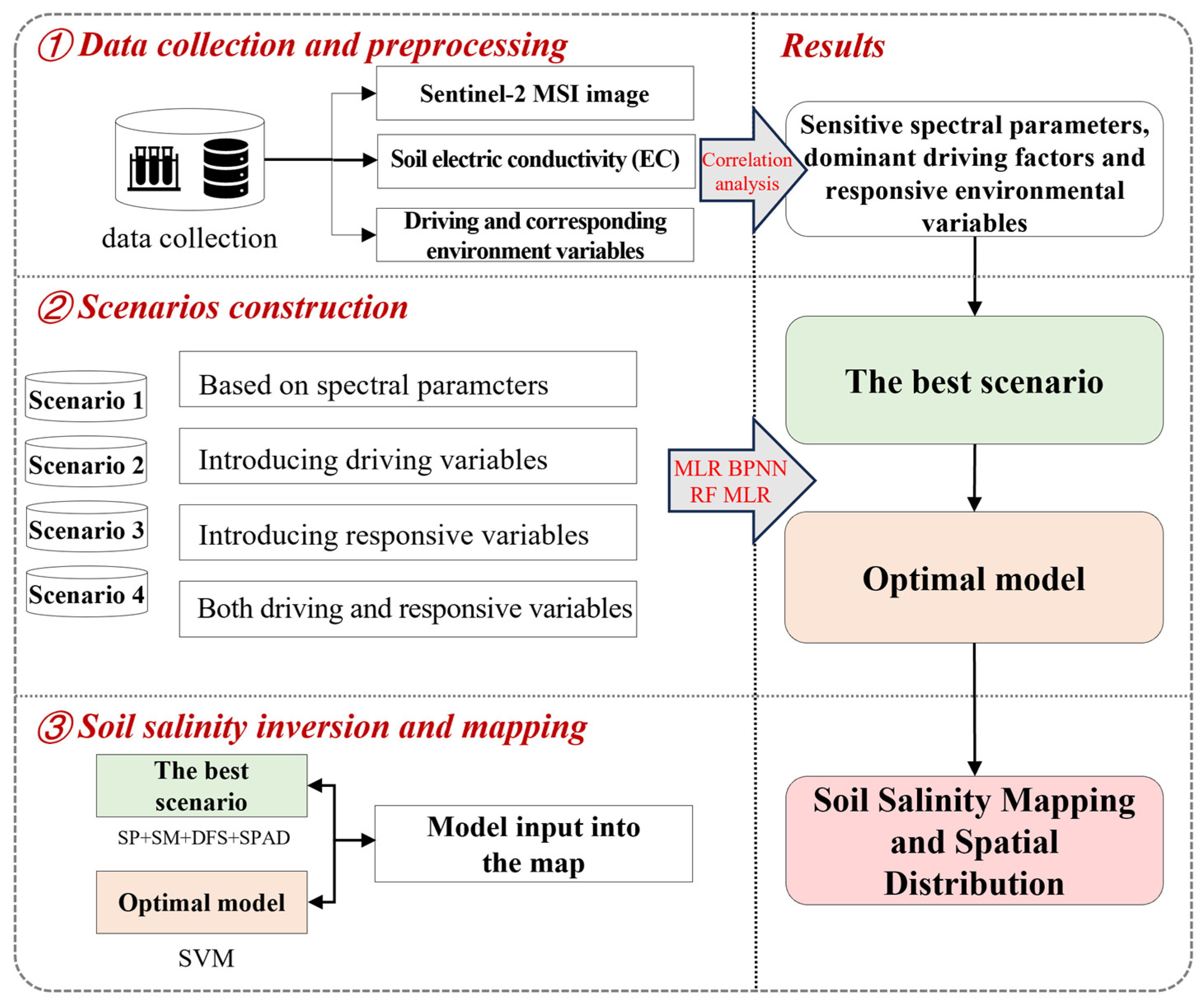
Initially, we examine sensitive spectral parameters related to soil salinity and determine the dominant environmental variables. Subsequently, these variables are then incorporated to build the inversion models from four scenarios: Scenario 1—spectral parameters only; Scenario 2—spectral parameters combined with driving variables; Scenario 3—spectral parameters combined with response variables; and Scenario 4—spectral parameters combined with both driving and response variables. Various modeling methods, including multiple linear regression (MLR) and Backpropagation Neural Network (BPNN), are employed. The performance and robustness of the different models are compared to determine the optimal model, with the aim of achieving accurate inversion and spatial distribution analysis of soil salinity in the Yellow River Delta. This study aims to identify the dominant driving and response variables affecting soil salinization and incorporate them to enhance the accuracy of soil salinity remote sensing inversion.

2.2. Study Area

The Yellow River Delta (E 118°40′–E 120°20′, N 37°25′–N 38°00′) is located in Eastern China, adjacent to the Bohai Sea at the estuary of the Yellow River Basin. Administered by Dongying City, Shandong Province, this region spans approximately 5450 square kilometers and features a temperate monsoon climate with flat topography, where elevation gradually declines from the Yellow River coastline to the surrounding areas. The dominant soils are coastal saline and alkaline types, and the agro-ecosystem is mainly composed of wheat, maize, and cotton, with natural vegetation such as reed and seepweed. Due to factors, such as shallow groundwater tables, seawater intrusion, groundwater contamination, and high rates of soil evaporation, the region experiences severe secondary salinization [30]. More than 80% of the cultivated land in the Yellow River Delta is affected by salinization, and soil salinity levels in some areas exceed 4 dS/m, classifying them as moderately to severely saline soils. This salinization has led to reduced crop vigor and increased mortality, resulting in low agricultural yields that hinder local agricultural development, exacerbate ecological degradation, and threaten regional security. This study focuses on a representative coastal saline–alkaline zone within the Yellow River Delta, specifically the Kenli District, Hekou District, and Lijin County in Shandong Province. The widespread and varying levels of salinization in this area make it an ideal research region, as illustrated in Figure 1.

2.3. Data Acquisition and Preprocessing

2.3.1. Field Sampling and Soil Salinity Measurement

In the study area, low spring precipitation combined with high evaporation promotes upward salt migration, resulting in elevated surface salinity and making the region representative of salinization processes. A total of 141 soil samples were collected from 15 to 17 May 2023, with 43, 56, and 42 samples collected on the respective days. Meteorological records confirmed no rainfall or irrigation during the period, ensuring stable surface salinity conditions. As a result, the electrical conductivity (EC) measurements obtained during this period are considered temporally stable and reflective of the true salinity conditions in the region. Soil surface EC measurements were conducted in situ at each sampling point, with three repeated readings taken and averaged to improve accuracy. Before measurement, surface debris was carefully removed to avoid interference. The EC110 device was calibrated daily following the manufacturer’s guidelines to ensure measurement reliability. The coordinates of each sampling point were recorded using a Trimble GEO 7X handheld differential GPS (Trimble Inc., Sunnyvale, CA, USA), and site information such as land use and crop condition was documented. The 141 samples were evenly distributed across the study area, covering a range of salinity gradients and land use types, with denser coverage in coastal zones prone to salinization.

2.3.2. Acquisition of Driving Variables

Based on the identified drivers of soil salinization in the Yellow River Delta and supported by the existing literature, the following variables were identified: precipitation (PRE), soil moisture (SM), distance from the sea (DFS), and ground elevation (GEL). Soil moisture was measured concurrently during sampling using a portable soil moisture meter. The distance from the sea was calculated using the nearest neighbor analysis function in ArcGIS to determine the shortest distance between the sampling points and the coastline. Ground elevation data were obtained from GEO 7X handheld GPS readings at the sampling points. Precipitation data were sourced from the OpenLandMap dataset.

2.3.3. Measurement of Response Variables

During sampling, the predominant crop in the study area was wheat. Two response variables—chlorophyll content (SPAD) and leaf area index (LAI)—were measured. SPAD reflects the photosynthetic efficiency and nutritional status of plants, whereas LAI provides direct insights into crop canopy structure and biomass. These indicators are key indicators for evaluating wheat growth and are directly affected by soil salinization [31,32].
SPAD and LAI were assessed using a SPAD-502 handheld chlorophyll meter (Jiuzhou Shengxin Technology Co., Ltd., Beijing, China)and an LAI-2000 canopy analyzer (LI-COR Biosciences, Lincoln, NE, USA), respectively. For SPAD measurements, five wheat canopy leaves were randomly collected within a 0.5 m diameter circle around each sampling point, and the average value was recorded as the SPAD measurement for that point [33]. For LAI measurements, three random locations near each sampling point were evaluated, and the average value was recorded as the LAI for that point [34].
Among them, the raster data processing and sources of the environmental variables are shown in Table 1.

2.3.4. Acquisition and Preprocessing of Sentinel-2 MSI Imagery

Sentinel-2 MSI data were obtained from the Copernicus Open Access Hub (https://dataspace.copernicus.eu/, accessed on 5 September 2023). This study utilized Sentinel-2 Level-1C imagery acquired on 16 May 2023, covering the study area. This product is an atmospherically corrected surface reflectance dataset [35]. Data preprocessing was carried out in the Sentinel Application Platform (SNAP), including atmospheric correction, radiometric calibration, and subsequent clipping to the study area. To refine the images further, the Normalized Difference Vegetation Index (NDVI) was used to exclude water bodies and non-cultivated areas [36], such as urban and built-up land, resulting in the final Sentinel-2 MSI imagery for the study area.

2.4. Methodology

A detailed technical flowchart is presented in Figure 2.

2.4.1. Analysis of Soil Salinity Sensitive Bands and Spectral Parameters

The GPS coordinates of the sampling points were imported into ArcGIS to extract reflectance data for each spectral band. Subsequently, SPSS 19.0 was employed to examine the correlation between band reflectance and soil salinity, thereby identifying bands most sensitive to soil salinity based on correlation coefficients. The relative sensitivity and importance of each band were evaluated based on its correlation with EC. Spectral parameters were constructed by combining different band reflectance, either linearly or nonlinearly, to mitigate the impact of atmospheric effects and noise on soil spectral features [37]. Fifteen spectral parameters were developed based on the selected sensitive bands and various calculation methods from previous studies, as detailed in Table 2. The correlation between these spectral parameters and soil salinity was analyzed, and their importance was determined based on the Pearson correlation coefficients. To avoid multicollinearity, parameters with inter-correlation coefficients greater than 0.9 were excluded [38]. Finally, sensitive spectral parameters were selected based on the strength of the correlations and the results of the multicollinearity analysis.

2.4.2. Analysis of Dominant Environmental Variables for Soil Salinity

Environmental variables significantly impact soil salinity, although the degree of influence varies among different indicators [48]. In this study, variables are categorized as driving variables (e.g., PRE, SM, GEL) and response variables (e.g., SPAD, LAI) based on their role in the soil–vegetation–atmosphere system. Driving variables are those that directly affect the formation and transformation processes of soil salinization, while response variables reflect the physiological or phenological responses of vegetation to salt stress. Dominant environmental variables influencing soil salinity were identified based on Pearson correlation coefficients and statistical significance levels, in accordance with previous research findings [49]. Variables with lower correlation coefficients and significance levels are excluded, retaining only those with a substantial impact on soil salinity as dominant environmental variables for modeling, thereby enhancing model performance.

2.4.3. Construction and Validation of Soil Salinity Inversion Models

The 141 samples are sorted by their EC values and then sampled at a 2:1 ratio using systematic sampling (1 sample from every 3 for validation), with 94 samples used for modeling and 47 samples for validation. Performance was evaluated through hold-out validation and 5-fold cross-validation.
Model Construction
For the 94 samples used in modeling, soil salinity inversion models were constructed under four different scenarios, as outlined in Section 2.1, using four methods: multiple linear regression (MLR), Backpropagation Neural Network (BPNN), Random Forest (RF), and Support Vector Machine (SVM).
MLR is a statistical method for establishing relationships between a dependent variable and multiple independent variables, fitting the model directly from the data without the need for additional parameter adjustments. BPNN, a commonly used artificial neural network for classification and regression tasks, was configured with a learning rate of 0.01, 1000 iterations, and an error threshold of 1 × 10⁻⁶. RF is an ensemble learning method that constructs multiple decision trees for prediction, with 60 trees, a minimum leaf node count of 10, and Out-of-Bag (OOB) error estimation and feature importance calculation enabled. SVM uses kernel functions to implicitly map data into high-dimensional space, with C (penalty factor) set to 0.7, gamma (radial basis function parameter) set to 1.2, epsilon (epsilon parameter in ε-SVR) set to 0.01, and a radial basis function (RBF) kernel. All algorithms were implemented within the MATLAB programming environment.
Model Validation
The 47 validation samples were used to evaluate and assess the models. The model performance was measured using the coefficient of determination (R2) and Root Mean Square Error (RMSE). A model with an R2 value closer to 1 and a smaller RMSE indicates better overall performance.
R 2 = 1 i = 1 n y i y ^ i 2 i = 1 n y i y ¯ 2
R M S E = 1 n i = 1 n y i y ^ i 2
In the formula, y i represents the observed value; y ^ i is the predicted value; y ¯ denotes the mean of the observed values; and n refers to the number of observations.

2.4.4. Spatial Distribution Inversion and Accuracy Analysis of Soil Salinity in the Study Area

Using Sentinel-2 MSI imagery, environmental variable data, and the optimal model, soil salinity inversion for the study area was conducted with MATLAB 2021a software to generate a spatially explicit regional soil salinity map. Based on previous research and coastal sodium chloride-type soil salinization classification standards [50], the inversion results were categorized into five levels, non-saline soil (<0.7 ms/cm), mild saline soil (0.7–1.5 ms/cm), moderate saline soil (1.5–3.0 ms/cm), severe saline soil (3.0–3.5 ms/cm), and solonchak (>3.5 ms/cm), creating a regional soil salinity classification map. Additionally, soil salinity at sampling points was interpolated using the inverse distance weighting method and compared with the inversion results to assess model accuracy.

3. Results and Analysis

3.1. Salinity Data of the Soil Samples

Descriptive statistical analysis of soil salinity data from the samples was conducted, and the results are presented in Table 3. The minimum EC in the study area is 0.01 ms/cm, while the maximum is 4.21 ms/cm. The average EC is 1.37 ms/cm, with a standard deviation of 0.8 ms/cm. Overall, the soil salinity levels are relatively high and exhibit a clear spatial gradient. The sample distribution is fairly uniform across the study area. Furthermore, the calibration and validation datasets show similar statistical characteristics, ensuring the representativeness of the samples and minimizing potential bias during model calibration and validation.

3.2. Sensitive Bands and Spectral Parameters of Soil Salinity

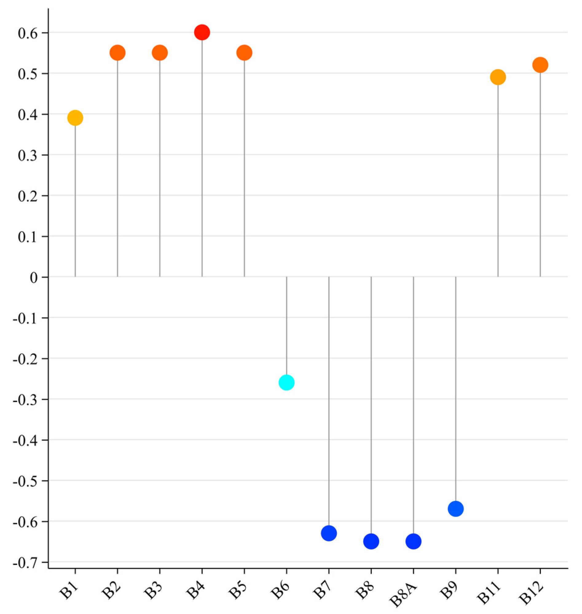
The correlation coefficients between EC and the single-band reflectance of Sentinel-2 MSI imagery range from −0.65 to 0.60, indicating generally strong associations. Specifically, bands B6, B7, B8, B8A, and B9 exhibited negative correlations, whereas the remaining bands showed positive correlations (see Figure 3). Based on the strength of these correlations and previous studies [50], bands with correlation coefficients greater than 0.55 or less than −0.65 are identified as sensitive bands for soil salinity. These included bands B2, B3, B4, B5, B8, and B8A.
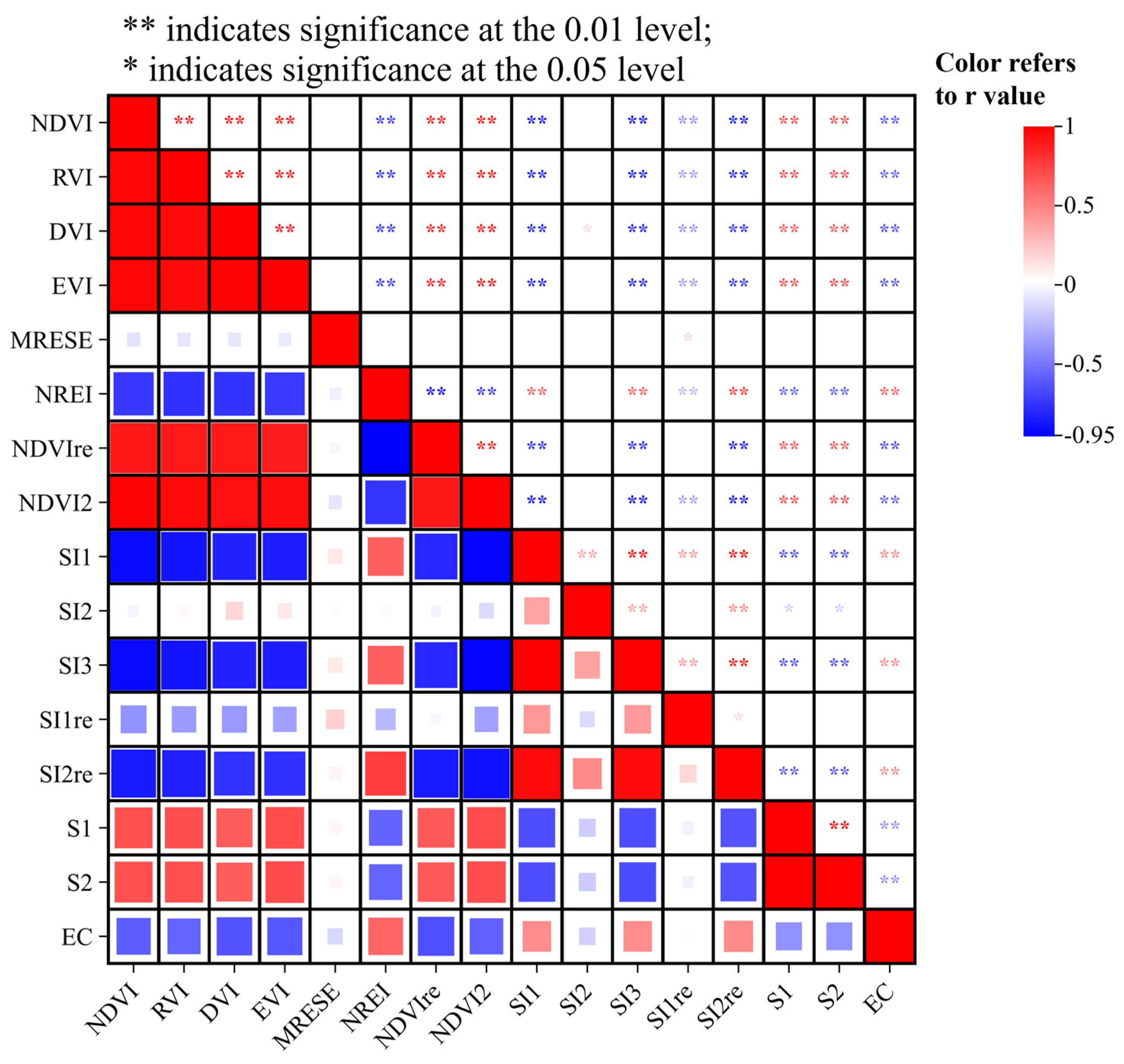
Using the selected sensitive bands, 15 spectral indices were generated through various mathematical transformations. Correlation analysis with measured EC showed that the Pearson correlation coefficients ranged from −0.65 to 0.65, with most indices showing enhanced correlations compared to the original bands (see Figure 4). An initial screening was performed to retain indices with higher relevance to soil salinity.
To address multicollinearity and enhance model stability and interpretability, Variance Inflation Factor (VIF) analysis was conducted. VIF is a common diagnostic tool to detect multivariate collinearity. Indices with VIF values exceeding 5 were excluded to reduce redundancy and prevent overfitting [51]. Following this filtering, the final set of indices included DVI, EVI, NREI, and NDVIre, which exhibited both strong correlations with EC and acceptable multicollinearity levels.

3.3. Selection of Dominant Environmental Variables of Soil Salinity

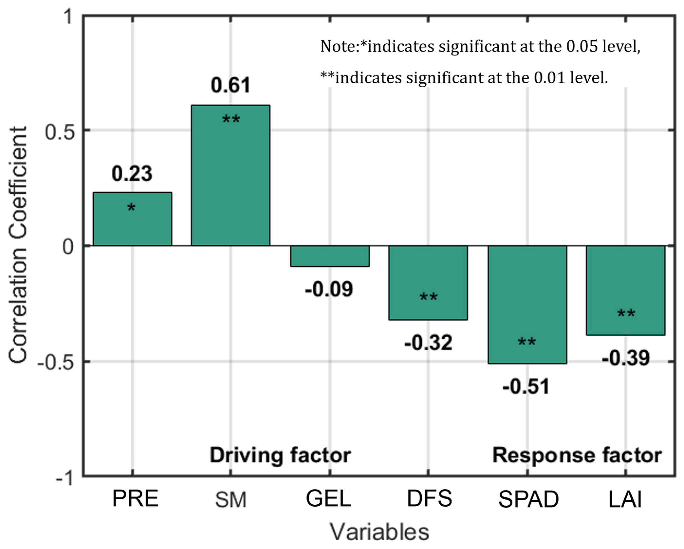
The correlation between EC and four driving factors—PRE, SM, GEL, and DFS—as well as two response variables—SPAD and LAI—is illustrated in Figure 5. The absolute values of the correlation coefficients for these six factors range from 0.09 to 0.61. Among them, four factors, excluding PRE and GEL, demonstrate strong correlation with soil salinity and pass the significance test. Specifically, SM shows the highest correlation coefficient at 0.61, followed by DFS with a coefficient of −0.32. PRE and GEL show weaker correlations, with absolute values below 0.3. Both response variables also display strong correlations with soil salinity, with SPAD at −0.51 and LAI at −0.39.
In summary, the dominant environmental variables influencing soil salinity are SM, DFS, SPAD, and LAI.

3.4. Quantitative Inversion Models of Soil Salinity

3.4.1. Soil Salinity Inversion Models Based on Scenario 1 (Only on Spectral Parameters)

Soil salinity inversion models were developed using four different algorithms, utilizing only the selected sensitive spectral parameters (SPs). The results are summarized in Table 4. Overall, the models exhibited moderate predictive capability, with R2 values ranging from 0.573 to 0.679 and RMSE values between 0.460 and 0.530 for the calibration set. For the validation set, R2 values ranged from 0.567 to 0.579, and RMSE values were between 0.506 and 0.513. Although these models based solely on spectral parameters were able to quantitatively estimate soil salinity, validation R2 values below 0.6 suggest that their robustness remains limited.
Among the four modeling methods, the RF model demonstrated the highest accuracy, followed by the BPNN, SVM, and MLR models. Specifically, the RF model achieved an R2 of 0.679 for the calibration set and 0.574 for the validation set, demonstrating the best predictive performance.

3.4.2. Soil Salinity Inversion Models Based on Scenario 2 (Spectral Parameters in Combination with Driving Variables)

In Scenario 2, SM and DFS as driving variables were integrated with SP to develop soil salinity inversion models, as detailed in Table 5.
When SM was combined with SP, the calibration set R2 values ranged from 0.637 to 0.696, with RMSE between 0.430 and 0.470. For the validation set, R2 values ranged from 0.601 to 0.653, and RMSE values ranged from 0.492 to 0.527. When DFS was combined with SP, the calibration set R2 values ranged from 0.623 to 0.667, with RMSE values ranging from 0.458 to 0.508. For the validation set, R2 values ranged from 0.628 to 0.656, and RMSE values ranged from 0.473 to 0.506. When both SM and DFS were integrated with SP, the model’s calibration set R2 values ranged from 0.691 to 0.771, with RMSE values between 0.388 and 0.434. For the validation set, R2 values ranged from 0.643 to 0.729, and RMSE values ranged from 0.407 to 0.498.
Overall, the inclusion of driving variables notably enhanced model stability and accuracy compared to models relying solely on spectral parameters. Specifically, models incorporating SM showed improvements in training set R2 by 0.017 to 0.073 and RMSE reductions of 0.03 to 0.065. Validation set R2 increased by 0.027 to 0.079, with RMSE decreasing by 0.009 to 0.014. The addition of DFS yielded mixed results, with training set R2 improving by 0.023 to 0.094 and validation set R2 by 0.05 to 0.089, though RMSE values for both sets slightly increased, indicating less consistent stability improvements. When both SM and DFS were combined, all four modeling approaches exhibited significant gains in both accuracy and stability: calibration set R2 increased by 0.017 to 0.177, RMSE decreased by 0.049 to 0.129, validation set R2 rose by 0.064 to 0.162, and RMSE decreased by 0.015 to 0.063. These results demonstrate that integrating SM and DFS as driving variables effectively enhances soil salinity inversion accuracy.
Among the four modeling methods incorporating both SM and DFS, the SVM model demonstrates the highest accuracy, followed by the MLR model, the RF model, and the BPNN model. Specifically, the SVM model achieves a calibration set R2 of 0.771 and a validation set R2 of 0.673, indicating the best predictive performance.

3.4.3. Soil Salinity Inversion Model Based on Scenario 3 (Spectral Parameters in Combination with Response Variables)

In Scenario 3, the response variables SPAD and LAI were incorporated alongside SP to develop soil salinity inversion models, as summarized in Table 6.
When SPAD was combined with SP, calibration set R2 values ranged from 0.657 to 0.688, with RMSE between 0.438 and 0.457. For the validation set, R2 ranged from 0.578 to 0.651, and RMSE from 0.462 to 0.542. When LAI was combined with SP, calibration R2 values were lower, ranging from 0.606 to 0.654, with RMSE ranging from 0.477 to 0.509. Validation set R2 values ranged from 0.544 to 0.626, and RMSE from 0.510 to 0.548. When both SPAD and LAI were integrated with SP, calibration set R2 ranged from 0.660 to 0.690, with RMSE between 0.435 and 0.487. Validation set R2 values ranged from 0.574 to 0.656, and RMSE from 0.478 to 0.545.
Overall, the impact of incorporating response variables on model accuracy and stability was variable. Adding SPAD generally improved model performance, with calibration set R2 increasing by 0.03 to 0.094 and RMSE decreasing by 0.02 to 0.073. For the validation set, R2 increased by 0.001 to 0.077, and RMSE decreased by 0.013 to 0.044. The improvement in model accuracy and stability from incorporating LAI is not significant, as no modeling method simultaneously improves both R2 and RMSE for both the calibration and validation sets. Incorporating both SPAD and LAI improves model accuracy and stability to some extent, with calibration set R2 increasing by 0.011 to 0.084 and RMSE decreasing by 0.016 to 0.073. For the validation set, R2 increased by 0.007 to 0.082, and RMSE decreased by 0.009 to 0.035. However, these enhancements were less pronounced compared to models incorporating only SPAD.
In summary, using SPAD alone or in combination with LAI led to improvements in model accuracy, with calibration set R2 values ranging from 0.657 to 0.688 and 0.660 to 0.690, respectively. Given the relatively small gain from adding LAI and the generally higher RMSE observed when both variables are included, it is recommended to use SPAD alone to maintain model simplicity and avoid unnecessary redundancy.
Among the four modeling methods that include SPAD, the SVM model exhibits the highest accuracy, followed by the BPNN, RF, and MLR models. The SVM model achieves a calibration set R2 of 0.688 and a validation set R2 of 0.634, demonstrating the best predictive performance.

3.4.4. Soil Salinity Inversion Model Based on Scenario 4 (Spectral Parameters in Combination with Both Driving and Response Variables)

Building upon the results from Scenarios 2 and 3, a soil salinity inversion model was developed by incorporating SP along with driving variables such as SM and DFS, as well as the response variable SPAD. The results are summarized in Table 7. Overall, the model demonstrated strong performance, with R2 values for the calibration set ranging from 0.750 to 0.813 and RMSE values from 0.351 to 0.390. For the validation set, R2 values ranged from 0.650 to 0.722, and RMSE values ranged from 0.409 to 0.494.
The inclusion of both driving and response variables substantially improved model accuracy and stability compared to models that did not incorporate these variables. Specifically, R2 values for the calibration set increased by 0.071 to 0.219, and RMSE decreased by 0.070 to 0.166. For the validation set, R2 values rose by 0.071 to 0.149, and RMSE decreased by 0.019 to 0.097. These improvements highlight the significant contribution of both driving and response variables in enhancing the model’s ability to invert soil salinity accurately.
Among the four modeling methods, the SVM model achieved the highest accuracy, followed by the BPNN, MLR, and RF models. Specifically, the SVM model attained an R2 of 0.813 for the calibration set and 0.722 for the validation set, demonstrating the best overall performance.

3.4.5. Model Comparison and Optimization

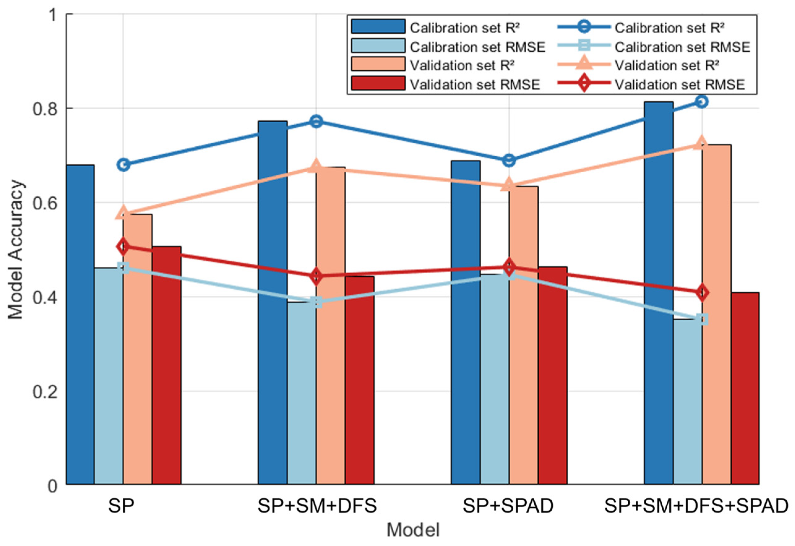
The performance and improvements of the best models under each scenario are illustrated in Figure 6. Overall, the models demonstrated strong predictive capability and stability, with calibration R2 values ranging from 0.679 to 0.813 and RMSE from 0.351 to 0.460. For the validation set, R2 values ranged from 0.574 to 0.722, and RMSE values ranged from 0.409 to 0.506. Notably, the optimal models in Scenarios 2, 3, and 4 all showed enhancements in both accuracy and stability compared to Scenario 1. Specifically, calibration R2 increased by 0.009 to 0.134 and RMSE decreased by 0.014 to 0.109. For the validation set, R2 improved by 0.060 to 0.148, while RMSE decreased by 0.044 to 0.097. These results confirm that incorporating environmental variables significantly enhances model performance.
Comparing the four scenarios, Scenario 4 achieves the highest model accuracy, followed by Scenario 2, Scenario 3, and Scenario 1, which has the lowest accuracy. Compared to Scenario 1, which does not incorporate environmental variables, Scenario 2 shows an increase in R2 at 0.092, indicating a moderate improvement in model accuracy. Scenario 3 demonstrates a minimal increase in R2 of 0.009, reflecting limited enhancement in accuracy. Notably, Scenario 4 exhibits the highest R2 increase of 0.134, indicating a significant improvement in model accuracy.
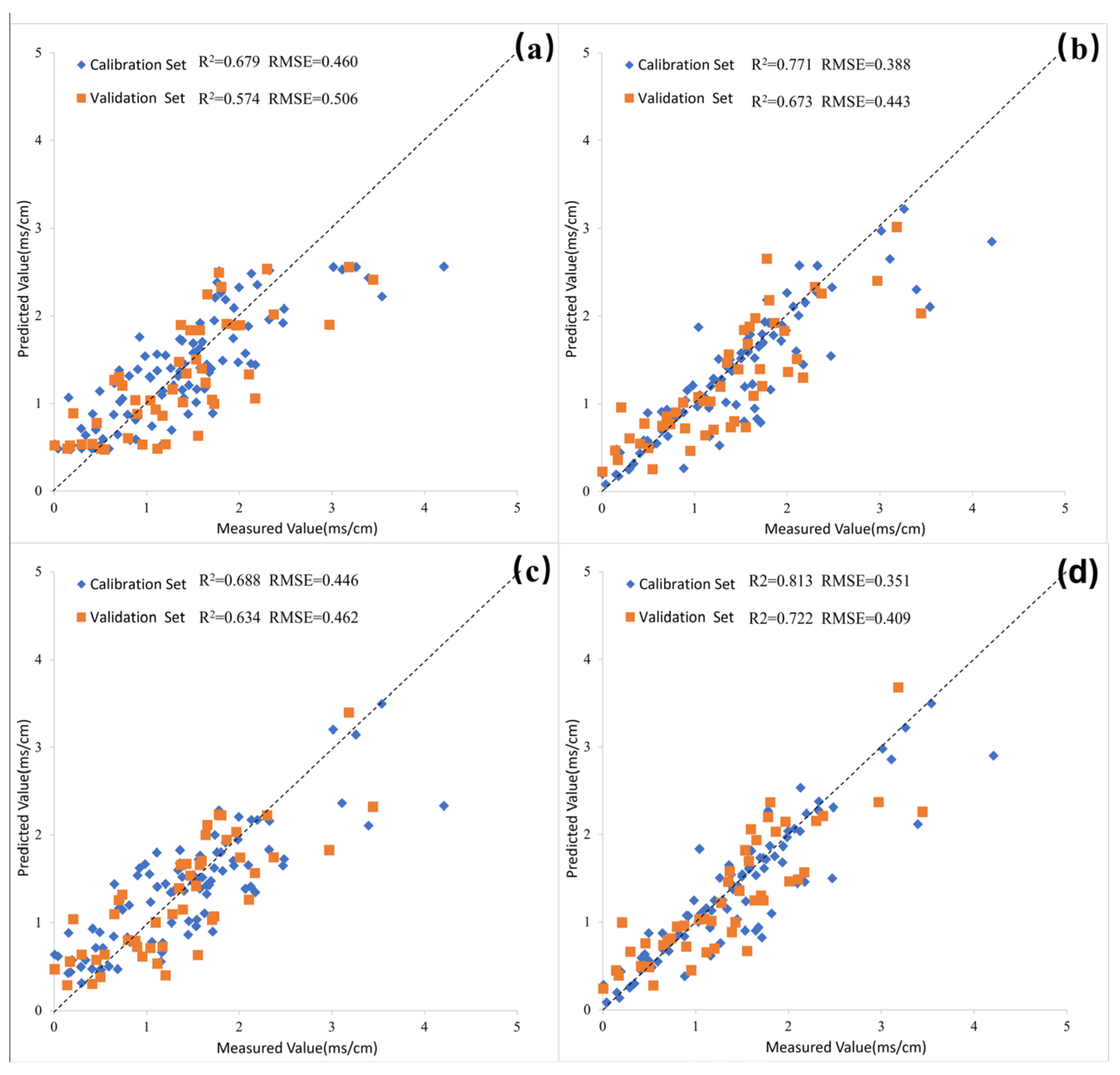
Figure 7 further illustrates the calibration and validation accuracy of the best models in each scenario. All models exhibit a strong linear relationship between observed and predicted values, with points evenly distributed along both sides of the 1:1 reference line, indicating reliable predictive performance. Among them, the model from Scenario 4 displays the most uniform and concentrated distribution around the line, confirming its superior prediction accuracy and establishing it as the optimal modeling approach for soil salinity inversion.

3.5. Soil Salinity Spatial Distribution Inversion and Accuracy Validation

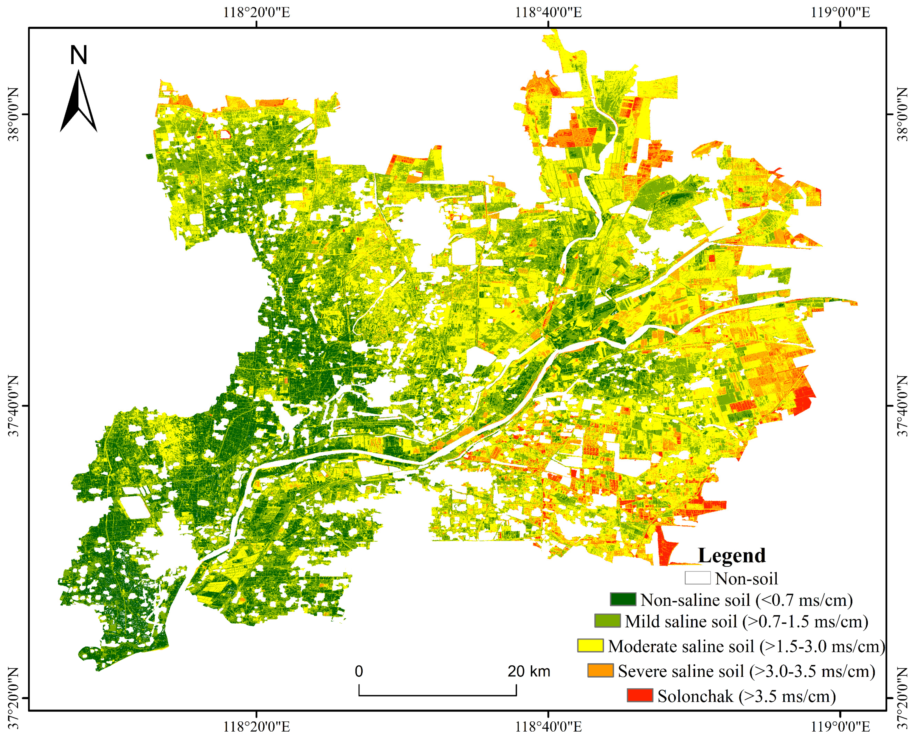
Based on the optimal model (SP + SM + DFS + SPAD), soil salinity inversion was performed for the study area (see Figure 8). The inversion results showed EC values ranging from 0 to 13.42 ms/cm, with an average of 1.55 ms/cm. This mean value closely aligns with the sample statistics, confirming the accuracy and robustness of the inversion model.
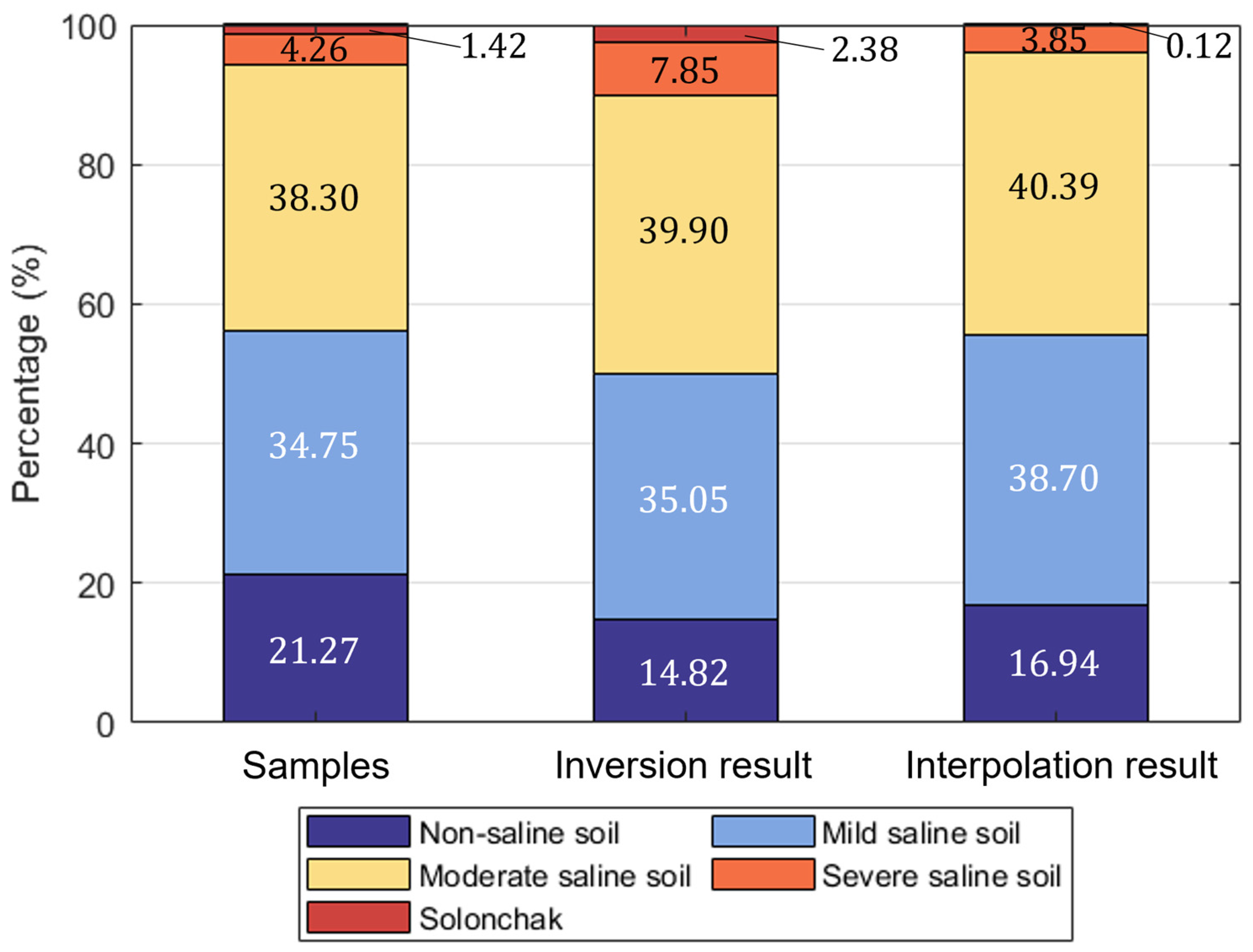
The spatial distribution of soil salinity levels is summarized in Figure 8. Moderate salinity levels dominate the study area, accounting for the largest proportion at 39.90%, followed by mildly saline soils at 35.05%. Non-saline soils comprise 14.82%, while severely saline soils and solonchak represent 7.85% and 2.38% of the area, respectively. These findings provide a clear overview of the salinization status in the Yellow River Delta and highlight the effectiveness of the inversion model in capturing spatial variability in soil salinity.
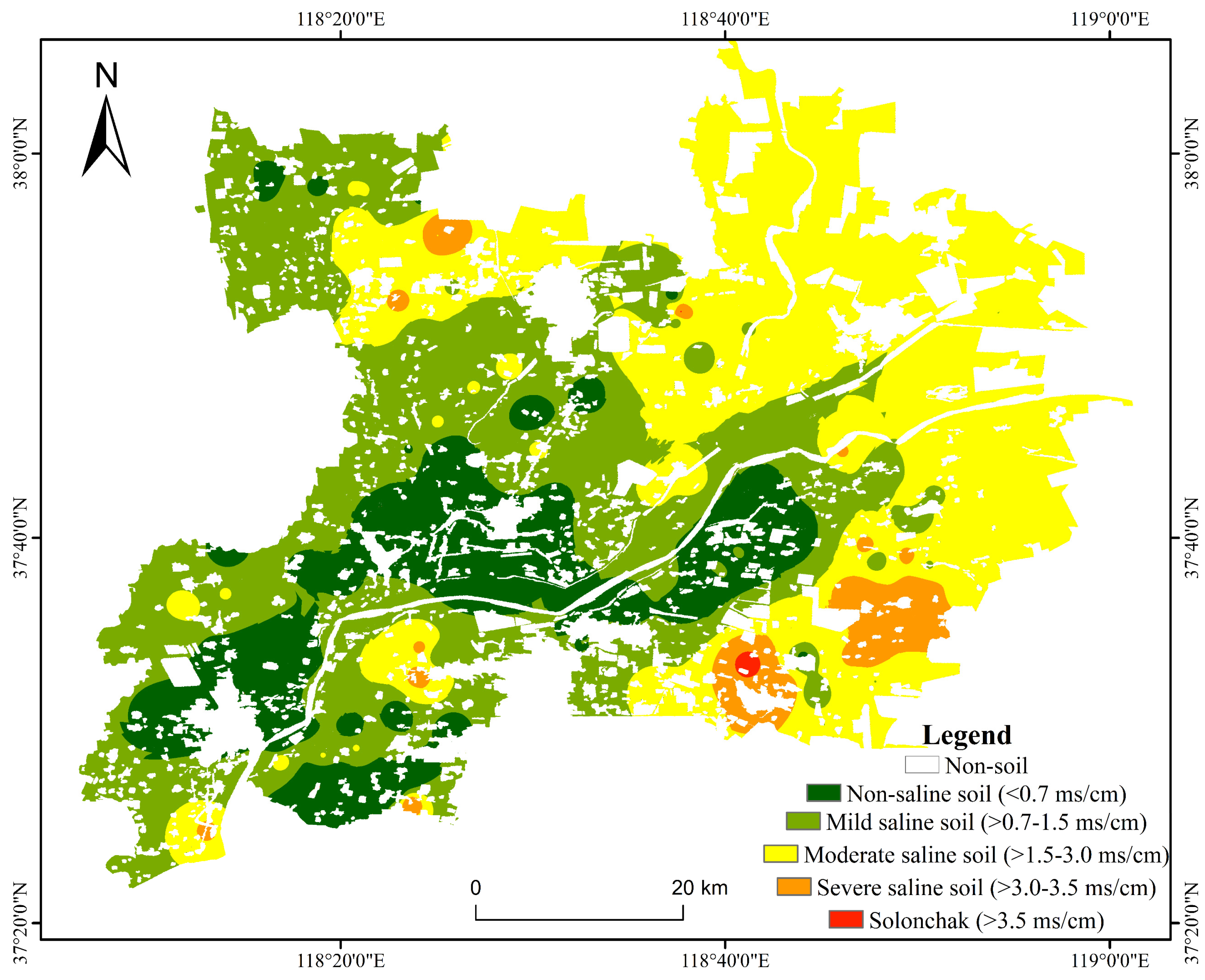
To validate the accuracy of the optimal model, the inverse distance weighting (IDW) method was employed to interpolate EC values at sample points, generating a soil salinity interpolation map (Figure 9) and illustrating the statistical distribution of salinization levels (Figure 10).
Among the sample points, moderate saline soils accounted for 38.30%, non-saline and mild saline soils made up 56.02%, and severe saline soils and solonchaks represented 5.68%. In the interpolation results, moderate saline soils accounted for 40.39%, non-saline and mild saline soils for 55.64%, and severe saline soils and solonchaks for 3.97%. In the inversion results, moderate saline soils made up 39.90%, non-saline and mild saline soils 49.87%, and severe saline soils and solonchaks 10.23%. In terms of spatial distribution, the interpolation map shows that non-saline soils are primarily located in the southwestern inland areas and along the Yellow River. Mild saline soils are distributed in the western part of the study area, moderate saline soils are found near the eastern coastal regions, and severe saline soils and solonchaks are concentrated along the coastline. These findings exhibit a high degree of spatial consistency with the inversion results. The inversion model demonstrated strong alignment with the sample measurements and the interpolation results, confirming its effectiveness in predicting regional soil salinity.

3.6. Characteristics of Soil Salinity Spatial Distribution

Based on the soil salinity distribution map of the Yellow River Delta region generated from the optimal model (Figure 8), it can be observed that soil salinity generally decreases from the eastern coastal areas toward the southwestern inland areas. Moderate saline soils, which constitute the largest proportion, are primarily concentrated in the northern and eastern coastal zones. Mild saline soils are more widely distributed and scattered throughout the entire region. Non-saline soils are mainly located in the southwestern part of the study area and along the banks of the Yellow River, showing the highest concentration in the southwestern inland zone. In contrast, severe saline soils and solonchak are predominantly found along the coastline. Overall, soil salinization in the Yellow River Delta is widespread, with the spatial distribution showing an increase in salinity along the coastline and a decrease along the Yellow River. Salinization is present at all levels, with moderate and mild saline soils being the most prevalent, which aligns with the actual conditions.

4. Discussion

4.1. Effectiveness of the Models Introducing Environmental Variables Under Various Scenarios

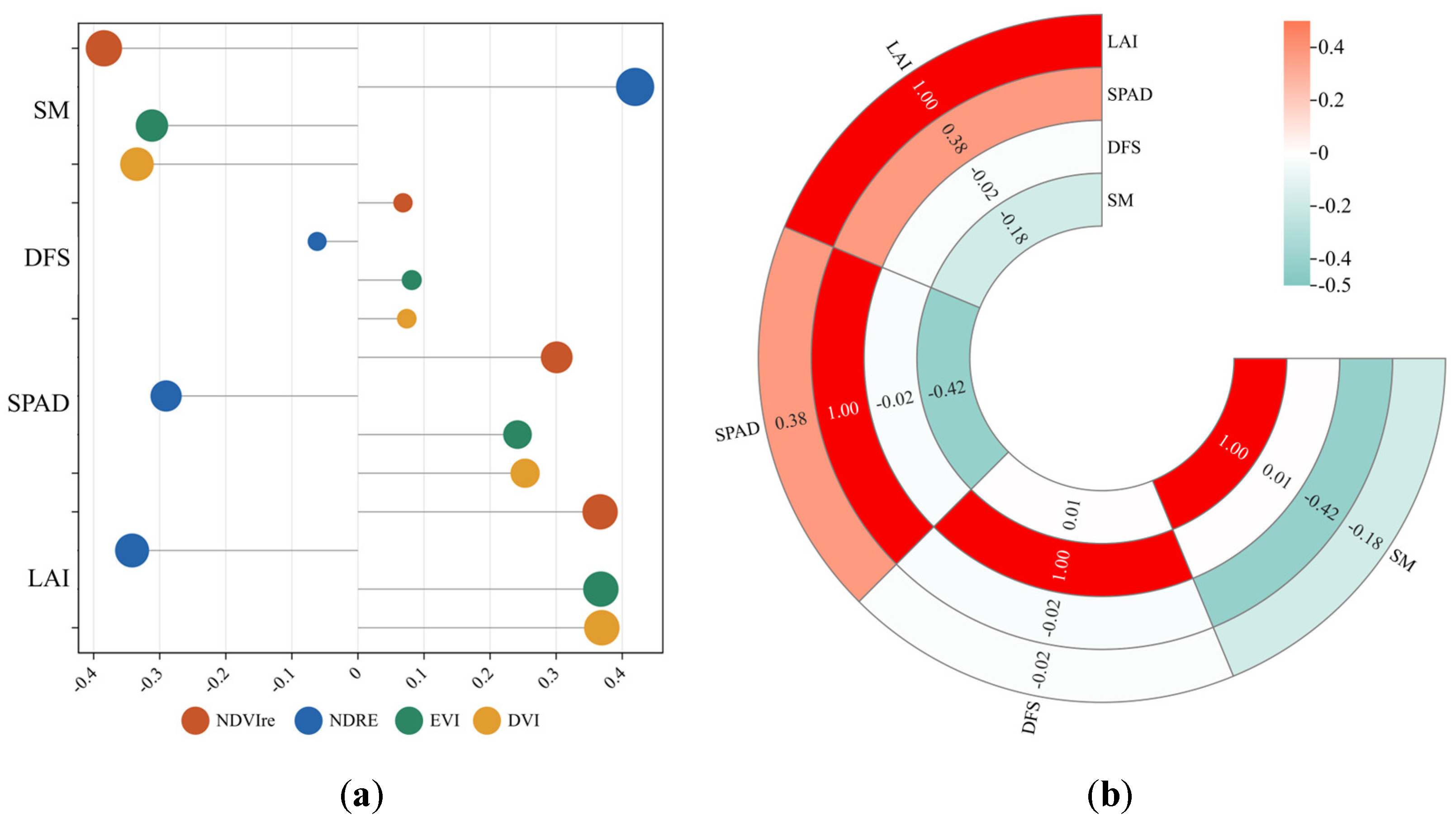
In this study, soil salinity inversion models were constructed under multiple scenarios to examine the impact of environmental variables on model accuracy. The results indicate that model accuracy varies across different scenarios, with notable improvement observed when both driving and response environmental variables are incorporated. To further explore the effectiveness of environmental variables in these scenarios, two types of correlations were analyzed: (a) correlations between dominant environmental variables and spectral parameters (SP) used in modeling, and (b) inter-correlations among the dominant environmental variables, as illustrated in Figure 11.
In Scenario 2, model accuracy ranks from high to low as follows: SP + SM + DFS > SP + DFS > SP + SM. Although soil moisture (SM) has a high correlation with soil salinity (0.61), Figure 11a shows that the absolute correlation coefficient between SM and spectral parameters (SPs) ranges from 0.31 to 0.42, which indicates that SPs can partially reflect SM variations. Thus, the additional information provided by introducing SM alone contributes minimally to soil salinity prediction, and its impact on model accuracy is limited. This observation aligns with the findings from Liu et al., who demonstrated a significant correlation between spectral reflectance and soil moisture within the 400–2500 nm range, suggesting that spectral reflectance effectively represents soil moisture content [52]. Additionally, SM experiences significant short-term fluctuations due to factors like rainfall, irrigation, and evaporation, resulting in high temporal variability [53]. This transient behavior may not effectively capture the stable patterns associated with salinity distribution [54]. From the perspective of hydrology, soil moisture directly affects salt transport through infiltration, leaching, and capillary rise [55]. Wet conditions may dilute or wash salts downward, while dry periods often promote upward salt movement via evaporation [56]. As a result, introducing SM alone has limited impact on improving model accuracy. Consequently, introducing SM alone has limited impact on improving model accuracy. In contrast, DFS shows relatively low correlation with SPs and contributes unique environmental information that SPs alone cannot capture. As a stable geographic attribute, DFS has a long-term and consistent influence on soil salinity [57]. Although DFS does not directly or immediately affect soil salinity distribution, its enduring environmental effect provides essential macro-level contextual information in modeling [58]. This observation is consistent with the findings of Zhao et al. [59], who found that DFS affects regional climate, groundwater levels, and groundwater mineralization, all of which play a significant role in soil salinity formation and accumulation. Thus, incorporating DFS into the model improves accuracy better than introducing SM alone. Furthermore, introducing both SM and DFS enables the model to capture complementary influences across different temporal dimensions, providing a more comprehensive explanation of soil salinity. Moreover, as shown in Figure 11b, the correlation between SM and DFS is very low (0.006), indicating minimal overlap in the environmental information provided by these two driving variables. Consequently, incorporating both SM and DFS avoids redundancy and enables a multidimensional representation of soil salinity spatial distribution, significantly enhancing model accuracy.
In Scenario 3, model accuracy ranks from high to low as follows: SP + SPAD > SP + SPAD + LAI > SP + LAI. SPAD directly reflects chlorophyll content, which is highly sensitive to salt stress, with a correlation coefficient of −0.51 relative to soil salinity. For example, Shah et al. demonstrated that under salt stress, chlorophyll content often decreases, enabling SPAD to effectively capture the direct effects of salinity on plant physiological conditions [60]. Furthermore, as shown in Figure 11a, the absolute correlation coefficient between SPAD and SPs remains relatively low (all below 0.3), indicating that including both spectral data and SPAD in the model does not introduce data redundancy, thereby effectively improving model accuracy. In contrast, LAI reflects vegetation coverage or leaf growth, which has a weaker correlation with soil salinity. Xu et al. found that LAI is influenced by various factors and is less sensitive to salinity, so incorporating LAI alone contributes minimally to model accuracy [61]. Additionally, the absolute correlation between LAI and SPs is relatively high, ranging from 0.36 to 0.37, suggesting that LAI provides limited independent information. This aligns with findings from Darvishzadeh et al., who demonstrated a strong correlation between LAI and vegetation spectral information, achieving high-accuracy LAI estimations using five vegetation spectral indices [62]. Therefore, including LAI alone does not significantly enhance model performance. As both SPAD and LAI are included, the primary effects of salinity are already captured by SPAD, making LAI’s contribution relatively minor, thus limiting any further improvement in model accuracy [59]. Additionally, Figure 11b shows that the correlation coefficient between SPAD and LAI is as high as 0.375, indicating a degree of information overlap. This redundancy increases model complexity and may lead to overfitting, potentially constraining improvements in predictive accuracy. Kulig et al. also reported a strong correlation between LAI and SPAD across various cultivation systems [63].
In Scenario 4, LAI was not included due to its relatively low correlation with soil salinity and information redundancy with SPAD. Therefore, this scenario integrates SPs, SM, and DFS from Scenario 2, along with SPAD from Scenario 3, to construct a more comprehensive yet efficient model. This combination allows the model to encompass both environmental background information and specific growth status data [64]. Together, these factors minimize information redundancy, enhancing the model interpretability and predictive accuracy.

4.2. Dominant Environmental Variables of Soil Salinity

Regarding soil salinity in the study area, the results indicate that the primary driving environmental variables are SM and DFS, while the dominant response variables are SPAD and LAI. These findings align with a substantial body of prior research. SM plays a critical role in both the dissolution and transport of soil salts. Zhu et al. demonstrated that higher soil moisture content facilitates the dissolution and migration of salts, thereby altering the distribution and concentration of soil salinity [65]. DFS can influence soil salinity through groundwater levels and seawater intrusion [66,67]. Metternich and Zinck demonstrated that coastal areas have elevated groundwater levels and are significantly affected by seawater intrusion, leading to higher groundwater salinity. Through capillary action, this salinity rises to the soil surface, increasing soil salinity. In contrast, areas farther from the sea are less influenced by seawater, resulting in lower groundwater and soil salinity levels [68]. The study area, situated in the Yellow River Delta adjacent to the Bohai Sea, experiences relatively low groundwater levels; thus, both soil moisture and distance from the sea exert distinct and significant influences on soil salinity, qualifying them as dominant driving variables.
Soil salinization not only inhibits overall plant growth but also adversely affects photosynthetic capacity and physiological functions [69]. In severe salinization conditions, salt accumulation leads to osmotic stress and ion toxicity, disrupting the photosynthesis process in leaf cells and causing degradation or inhibited synthesis of chlorophyll, ultimately resulting in a decrease in SPAD values. Feng et al. confirmed that SPAD values significantly decrease in severe salinization, reflecting the negative impact of salt stress on photosynthesis [70]. Additionally, soil salinity significantly suppresses LAI. Salt stress impairs plant water uptake, leading to physiological disturbances that hinder leaf development and reduce LAI. Yasir et al. demonstrated that salt stress markedly decreases leaf area and overall plant growth by lowering osmotic potential and causing ion toxicity, ultimately impacting crop LAI [71].

4.3. Limitations and Outlook

Research has shown that machine learning models typically require large training datasets—often comprising hundreds to thousands of samples—to achieve robust generalizability and mitigate overfitting [72]. Although the sample size in this study was relatively small, it met the conventional requirements for remote sensing inversion modeling, and the model achieved satisfactory accuracy [73]. This indicates that the selected environmental variables and model structure were effective to a certain extent. Additionally, expanding the sample size in future work could further enhance model robustness and reduce potential biases arising from limited data.
Moreover, this study primarily incorporated numerical environmental variables such as soil moisture, distance from the sea, and chlorophyll content. The existing literature suggests that non-numerical factors, such as land cover type, land use type, and crop type, also significantly influence soil salinity distribution [74]. However, effective methods for integrating such categorical variables into quantitative inversion models remain underdeveloped. Future research should focus on exploring approaches to incorporate non-numerical variables to improve both the accuracy and interpretability of soil salinity inversion models.

5. Conclusions

This study, utilizing Sentinel-2 MSI imagery, established four distinct scenarios and developed a method for soil salinity remote sensing inversion that integrates both driving and response environmental variables. The results show that DVI, EVI, NREI, and NDVIre are sensitive spectral parameters, while SM and DFS are the dominant driving variables, and SPAD and LAI are key response variables. The incorporation of either category of environmental variables improved model accuracy, with the greatest enhancement observed when both were combined. The suitable model, integrating SM, DFS, and SPAD, achieved the best performance, particularly using the SVM method. These findings confirm that combining spectral, driving, and response variables enhances inversion accuracy and reduces the lag effects associated with vegetation indicators. The proposed method offers a practical framework for improving soil salinity monitoring in coastal areas, providing valuable guidance for salinization management and precision agriculture. By accurately mapping salinity levels, it supports the development of adaptive strategies, such as optimizing irrigation, introduction of salt-tolerant crops, and implementation of drainage systems.

Author Contributions

Conceptualization, Q.Z. and H.C.; methodology, Q.Z.; software, Q.Z. and D.W.; validation, Y.Z.; formal analysis, Q.Z. and D.W.; investigation, Y.Z. and Z.L.; resources, Y.Z.; data curation, Z.L.; writing—original draft preparation, Q.Z.; writing—review and editing, Q.Z., D.W. and H.C.; visualization, Q.Z.; supervision, H.C.; project administration, H.C.; funding acquisition, H.C. and P.L. All authors have read and agreed to the published version of the manuscript.

Funding

This research was supported by the National Natural Science Foundation of China [grant number 42477523], the Natural Science Foundation of Shandong Province of China [grant number ZR2023MD033] the National Key Research and Development Program of China [grant number 2023YFD2303304].

Data Availability Statement

The data presented in this study are available on request from the corresponding author. The data are not publicly available due to privacy.

Acknowledgments

Thanks to the ESA for support with the Sentinel-2A MSI images.

Conflicts of Interest

The authors declare no conflicts of interest.

References

  1. Zhao, C.; Zhang, H.; Song, C.; Zhu, J.-K.; Shabala, S. Mechanisms of Plant Responses and Adaptation to Soil Salinity. Innovation 2020, 1, 100017. [Google Scholar] [CrossRef] [PubMed]
  2. Chen, H.; Zhao, G.; Li, Y.; Wang, D.; Ma, Y. Monitoring the Seasonal Dynamics of Soil Salinization in the Yellow River Delta of China Using Landsat Data. Nat. Hazards Earth Syst. Sci. 2019, 19, 1499–1508. [Google Scholar] [CrossRef]
  3. Nouri, H.; Borujeni, S.C.; Nirola, R.; Hassanli, A.; Beecham, S.; Alaghmand, S.; Saint, C.; Mulcahy, D. Application of Green Remediation on Soil Salinity Treatment: A Review on Halophytoremediation. Process Saf. Environ. Prot. 2017, 107, 94–107. [Google Scholar] [CrossRef]
  4. Hassani, A.; Azapagic, A.; Shokri, N. Predicting Long-Term Dynamics of Soil Salinity and Sodicity on a Global Scale. Proc. Natl. Acad. Sci. USA 2020, 117, 33017–33027. [Google Scholar] [CrossRef]
  5. Wang, Z.; Zhao, G.; Gao, M.; Chang, C. Spatial Variability of Soil Salinity in Coastal Saline Soil at Different Scales in the Yellow River Delta, China. Environ. Monit. Assess. 2017, 189, 80. [Google Scholar] [CrossRef]
  6. Abd El-Hamid, H.T.; Hong, G. Hyperspectral Remote Sensing for Extraction of Soil Salinization in the Northern Region of Ningxia. Model. Earth Syst. Environ. 2020, 6, 2487–2493. [Google Scholar] [CrossRef]
  7. Daliakopoulos, I.N.; Tsanis, I.K.; Koutroulis, A.; Kourgialas, N.N.; Varouchakis, A.E.; Karatzas, G.P.; Ritsema, C.J. The Threat of Soil Salinity: A European Scale Review. Sci. Total Environ. 2016, 573, 727–739. [Google Scholar] [CrossRef]
  8. Guo, M.; Yang, L.; Zhang, L.; Shen, F.; Meadows, M.E.; Zhou, C. Hydrology, Vegetation, and Soil Properties as Key Drivers of Soil Organic Carbon in Coastal Wetlands: A High-Resolution Study. Environ. Sci. Ecotechnol. 2025, 23, 100482. [Google Scholar] [CrossRef]
  9. Taghadosi, M.M.; Hasanlou, M.; Eftekhari, K. Retrieval of Soil Salinity from Sentinel-2 Multispectral Imagery. Eur. J. Remote Sens. 2019, 52, 138–154. [Google Scholar] [CrossRef]
  10. Wang, Y.; Deng, C.; Liu, Y.; Niu, Z.; Li, Y. Identifying Change in Spatial Accumulation of Soil Salinity in an Inland River Watershed, China. Sci. Total Environ. 2018, 621, 177–185. [Google Scholar] [CrossRef]
  11. Eswar, D.; Karuppusamy, R.; Chellamuthu, S. Drivers of Soil Salinity and Their Correlation with Climate Change. Curr. Opin. Environ. Sustain. 2021, 50, 310–318. [Google Scholar] [CrossRef]
  12. Bennett, L.T.; Mele, P.M.; Annett, S.; Kasel, S. Examining Links between Soil Management, Soil Health, and Public Benefits in Agricultural Landscapes: An Australian Perspective. Agric. Ecosyst. Environ. 2010, 139, 1–12. [Google Scholar] [CrossRef]
  13. Zhang, Z.-X.; Song, Y.-T.; Zhang, H.-Z.; Li, X.-J.; Niu, B.-B. Spatiotemporal Dynamics of Soil Salinity in the Yellow River Delta under the Impacts of Hydrology and Climate. Ying Yong Sheng Tai Xue Bao= J. Appl. Ecol. 2021, 32, 1393–1405. [Google Scholar]
  14. Letey, J.; Hoffman, G.J.; Hopmans, J.W.; Grattan, S.R.; Suarez, D.; Corwin, D.L.; Oster, J.D.; Wu, L.; Amrhein, C. Evaluation of Soil Salinity Leaching Requirement Guidelines. Agric. Water Manag. 2011, 98, 502–506. [Google Scholar] [CrossRef]
  15. Nawar, S.; Buddenbaum, H.; Hill, J.; Kozak, J. Modeling and Mapping of Soil Salinity with Reflectance Spectroscopy and Landsat Data Using Two Quantitative Methods (PLSR and MARS). Remote Sens. 2014, 6, 10813–10834. [Google Scholar] [CrossRef]
  16. Wang, F.; Shi, Z.; Biswas, A.; Yang, S.; Ding, J. Multi-Algorithm Comparison for Predicting Soil Salinity. Geoderma 2020, 365, 114211. [Google Scholar] [CrossRef]
  17. Corwin, D.L. Climate Change Impacts on Soil Salinity in Agricultural Areas. Eur. J. Soil Sci. 2021, 72, 842–862. [Google Scholar] [CrossRef]
  18. Sultanov, M.; Ibrakhimov, M.; Akramkhanov, A.; Bauer, C.; Conrad, C. Modelling End-of-Season Soil Salinity in Irrigated Agriculture through Multi-Temporal Optical Remote Sensing, Environmental Parameters, and in Situ Information. PFG–J. Photogramm. Remote Sens. Geoinf. Sci. 2018, 86, 221–233. [Google Scholar] [CrossRef]
  19. Peng, J.; Biswas, A.; Jiang, Q.; Zhao, R.; Hu, J.; Hu, B.; Shi, Z. Estimating Soil Salinity from Remote Sensing and Terrain Data in Southern Xinjiang Province, China. Geoderma 2019, 337, 1309–1319. [Google Scholar] [CrossRef]
  20. Huang, H.; Liu, Y.; Liu, Y.; Tong, Z.; Ren, Z.; Xie, Y. Digital Mapping of Soil pH and Driving Factor Analysis Based on Environmental Variable Screening. Sustainability 2025, 17, 3173. [Google Scholar] [CrossRef]
  21. Li, Y.; Zheng, S.; Wang, L.; Dai, X.; Zang, D.; Qi, B.; Meng, X.; Mei, X.; Luo, C.; Liu, H. Systematic Identification of Factors Influencing the Spatial Distribution of Soil Organic Matter in Croplands within the Black Soil Region of Northeastern China across Multiple Scales. Catena 2025, 249, 108633. [Google Scholar] [CrossRef]
  22. Du, Z.; Gao, B.; Ou, C.; Du, Z.; Yang, J.; Batsaikhan, B.; Dorjgotov, B.; Yun, W.; Zhu, D. A Quantitative Analysis of Factors Influencing Organic Matter Concentration in the Topsoil of Black Soil in Northeast China Based on Spatial Heterogeneous Patterns. ISPRS Int. J. Geo-Inf. 2021, 10, 348. [Google Scholar] [CrossRef]
  23. Munns, R.; Cramer, G.R.; Ball, M.C. Interactions between Rising CO2, Soil Salinity, and Plant Growth. In Carbon Dioxide and Environmental Stress; Elsevier: Amsterdam, The Netherlands, 1999; pp. 139–167. [Google Scholar]
  24. Darwish, T.; Atallah, T.; El Moujabber, M.; Khatib, N. Salinity Evolution and Crop Response to Secondary Soil Salinity in Two Agro-Climatic Zones in Lebanon. Agric. Water Manag. 2005, 78, 152–164. [Google Scholar] [CrossRef]
  25. Haj-Amor, Z.; Araya, T.; Kim, D.-G.; Bouri, S.; Lee, J.; Ghiloufi, W.; Yang, Y.; Kang, H.; Jhariya, M.K.; Banerjee, A.; et al. Soil Salinity and Its Associated Effects on Soil Microorganisms, Greenhouse Gas Emissions, Crop Yield, Biodiversity and Desertification: A Review. Sci. Total Environ. 2022, 843, 156946. [Google Scholar] [CrossRef] [PubMed]
  26. Sahab, S.; Suhani, I.; Srivastava, V.; Chauhan, P.S.; Singh, R.P.; Prasad, V. Potential Risk Assessment of Soil Salinity to Agroecosystem Sustainability: Current Status and Management Strategies. Sci. Total Environ. 2021, 764, 144164. [Google Scholar] [CrossRef]
  27. Shi, X.; Song, J.; Wang, H.; Lv, X.; Tian, T.; Wang, J.; Li, W.; Zhong, M.; Jiang, M. Improving the Monitoring of Root Zone Soil Salinity under Vegetation Cover Conditions by Combining Canopy Spectral Information and Crop Growth Parameters. Front. Plant Sci. 2023, 14, 1171594. [Google Scholar] [CrossRef]
  28. Scudiero, E.; Skaggs, T.H.; Corwin, D.L. Regional-Scale Soil Salinity Assessment Using Landsat ETM+ Canopy Reflectance. Remote Sens. Environ. 2015, 169, 335–343. [Google Scholar] [CrossRef]
  29. Munns, R. Comparative Physiology of Salt and Water Stress. Plant Cell Environ. 2002, 25, 239–250. [Google Scholar] [CrossRef]
  30. Wen, Y.; Guo, B.; Zang, W.; Ge, D.; Luo, W.; Zhao, H. Desertification Detection Model in Naiman Banner Based on the Albedo-Modified Soil Adjusted Vegetation Index Feature Space Using the Landsat8 OLI Images. Geomat. Nat. Hazards Risk 2020, 11, 544–558. [Google Scholar] [CrossRef]
  31. Zhao, J.; Pan, F.; Xiao, X.; Hu, L.; Wang, X.; Yan, Y.; Zhang, S.; Tian, B.; Yu, H.; Lan, Y. Summer Maize Growth Estimation Based on Near-Surface Multi-Source Data. Agronomy 2023, 13, 532. [Google Scholar] [CrossRef]
  32. Ji, J.; Li, N.; Cui, H.; Li, Y.; Zhao, X.; Zhang, H.; Ma, H. Study on Monitoring SPAD Values for Multispatial Spatial Vertical Scales of Summer Maize Based on UAV Multispectral Remote Sensing. Agriculture 2023, 13, 1004. [Google Scholar] [CrossRef]
  33. Yuan, Z.; Cao, Q.; Zhang, K.; Ata-Ul-Karim, S.T.; Tian, Y.; Zhu, Y.; Cao, W.; Liu, X. Optimal Leaf Positions for SPAD Meter Measurement in Rice. Front. Plant Sci. 2016, 7, 719. [Google Scholar] [CrossRef] [PubMed]
  34. Liu, J.; Pattey, E.; Admiral, S. Assessment of in Situ Crop LAI Measurement Using Unidirectional View Digital Photography. Agric. For. Meteorol. 2013, 169, 25–34. [Google Scholar] [CrossRef]
  35. Su, W.; Zhang, M.; Jiang, K.; Zhu, D.; Huang, J.; Wang, P. Atmospheric Correction Method for Sentinel-2 Satellite Imagery. Acta Opt. Sin. 2018, 38, 0128001. [Google Scholar] [CrossRef]
  36. Bai, L.; Wang, C.; Zang, S.; Zhang, Y.; Hao, Q.; Wu, Y. Remote Sensing of Soil Alkalinity and Salinity in the Wuyu’er-Shuangyang River Basin, Northeast China. Remote Sens. 2016, 8, 163. [Google Scholar] [CrossRef]
  37. Yu, H.; Liu, M.; Du, B.; Wang, Z.; Hu, L.; Zhang, B. Mapping Soil Salinity/Sodicity by Using Landsat OLI Imagery and PLSR Algorithm over Semiarid West Jilin Province, China. Sensors 2018, 18, 1048. [Google Scholar] [CrossRef]
  38. Zhang, S.; Zhao, J.; Yang, J.; Xie, J.; Sun, Z. Feature Selection and Regression Models for Multisource Data-Based Soil Salinity Prediction: A Case Study of Minqin Oasis in Arid China. Land 2024, 13, 877. [Google Scholar] [CrossRef]
  39. Tucker, C.J. Red and Photographic Infrared Linear Combinations for Monitoring Vegetation. Remote Sens. Environ. 1979, 8, 127–150. [Google Scholar] [CrossRef]
  40. Foody, G.M.; Cutler, M.E.; McMorrow, J.; Pelz, D.; Tangki, H.; Boyd, D.S.; Douglas, I. Mapping the Biomass of Bornean Tropical Rain Forest from Remotely Sensed Data. Glob. Ecol. Biogeogr. 2001, 10, 379–387. [Google Scholar] [CrossRef]
  41. Vaglio Laurin, G.; Francini, S.; Luti, T.; Chirici, G.; Pirotti, F.; Papale, D. Satellite Open Data to Monitor Forest Damage Caused by Extreme Climate-Induced Events: A Case Study of the Vaia Storm in Northern Italy. For. Int. J. For. Res. 2021, 94, 407–416. [Google Scholar] [CrossRef]
  42. Kanke, Y.; Tubaña, B.; Dalen, M.; Harrell, D. Evaluation of Red and Red-Edge Reflectance-Based Vegetation Indices for Rice Biomass and Grain Yield Prediction Models in Paddy Fields. Precis. Agric. 2016, 17, 507–530. [Google Scholar] [CrossRef]
  43. Adamczyk, J.; Osberger, A. Red-Edge Vegetation Indices for Detecting and Assessing Disturbances in Norway Spruce Dominated Mountain Forests. Int. J. Appl. Earth Obs. Geoinf. 2015, 37, 90–99. [Google Scholar] [CrossRef]
  44. Yadav, V.P.; Prasad, R.; Bala, R.; Srivastava, P.K. Assessment of Red-Edge Vegetation Descriptors in a Modified Water Cloud Model for Forward Modelling Using Sentinel—1A and Sentinel—2 Satellite Data. Int. J. Remote Sens. 2021, 42, 794–804. [Google Scholar] [CrossRef]
  45. Delegido, J.; Verrelst, J.; Alonso, L.; Moreno, J. Evaluation of Sentinel-2 Red-Edge Bands for Empirical Estimation of Green LAI and Chlorophyll Content. Sensors 2011, 11, 7063–7081. [Google Scholar] [CrossRef] [PubMed]
  46. Nicolas, H.; Walter, C. Detecting Salinity Hazards within a Semiarid Context by Means of Combining Soil and Remote-Sensing Data. Geoderma 2006, 134, 217–230. [Google Scholar] [CrossRef]
  47. Wang, J.; Ding, J.; Yu, D.; Ma, X.; Zhang, Z.; Ge, X.; Teng, D.; Li, X.; Liang, J.; Lizaga, I.; et al. Capability of Sentinel-2 MSI Data for Monitoring and Mapping of Soil Salinity in Dry and Wet Seasons in the Ebinur Lake Region, Xinjiang, China. Geoderma 2019, 353, 172–187. [Google Scholar] [CrossRef]
  48. Zhao, W.; Ma, F.; Yu, H.; Li, Z. Inversion Model of Salt Content in Alfalfa-Covered Soil Based on a Combination of UAV Spectral and Texture Information. Agriculture 2023, 13, 1530. [Google Scholar] [CrossRef]
  49. Stavi, I.; Thevs, N.; Priori, S. Soil Salinity and Sodicity in Drylands: A Review of Causes, Effects, Monitoring, and Restoration Measures. Front. Environ. Sci. 2021, 9, 712831. [Google Scholar] [CrossRef]
  50. Ma, M.; Hao, Y.; Huang, Q.; Liu, Y.; Xiu, L.; Gao, Q. Soil Salinity Estimation by 3D Spectral Space Optimization and Deep Soil Investigation in the Songnen Plain, Northeast China. Sustainability 2024, 16, 2069. [Google Scholar] [CrossRef]
  51. Gerardo, R.; de Lima, I.P. Sentinel-2 Satellite Imagery-Based Assessment of Soil Salinity in Irrigated Rice Fields in Portugal. Agriculture 2022, 12, 1490. [Google Scholar] [CrossRef]
  52. Liu, W.; Frédéric, B.; Gu, X.; Tong, Q.; Zheng, L.; Zhang, B. Relating Soil Surface Moisture to Reflectance. Remote Sens. Environ. 2002, 81, 238–246. [Google Scholar]
  53. Rahmati, M.; Amelung, W.; Brogi, C.; Dari, J.; Flammini, A.; Bogena, H.; Brocca, L.; Chen, H.; Groh, J.; Koster, R.D.; et al. Soil Moisture Memory: State-of-the-art and the Way Forward. Rev. Geophys. 2024, 62, e2023RG000828. [Google Scholar] [CrossRef]
  54. Yin, D.; Song, X.; Zhu, X.; Guo, H.; Zhang, Y.; Zhang, Y. Spatiotemporal Analysis of Soil Moisture Variability and Its Driving Factor. Remote Sens. 2023, 15, 5768. [Google Scholar] [CrossRef]
  55. Nick, S.M.; Copty, N.K.; Saygın, S.D.; Öztürk, H.S.; Demirel, B.; Emadian, S.M.; Erpul, G.; Sedighi, M.; Babaei, M. Impact of Soil Compaction and Irrigation Practices on Salt Dynamics in the Presence of a Saline Shallow Groundwater: An Experimental and Modelling Study. Hydrol. Process. 2024, 38, e15135. [Google Scholar] [CrossRef]
  56. Kelln, C.; Barbour, S.L.; Qualizza, C. Controls on the spatial distribution of soil moisture and solute transport in a sloping reclamation cover. Can. Geotech. J. 2008, 45, 351–366. [Google Scholar] [CrossRef]
  57. Sun, G.; Zhu, Y.; Ye, M.; Yang, Y.; Yang, J.; Mao, W.; Wu, J. Regional Soil Salinity Spatiotemporal Dynamics and Improved Temporal Stability Analysis in Arid Agricultural Areas. J. Soils Sediments 2022, 22, 272–292. [Google Scholar] [CrossRef]
  58. Yurtseven, I.; Randhir, T.O. Multivariate Assessment of Spatial and Temporal Variations in Irrigation Water Quality in Lake Uluabat Watershed of Turkey. Environ. Monit. Assess. 2020, 192, 793. [Google Scholar] [CrossRef]
  59. Zhao, X.; Xi, H.; Yu, T.; Cheng, W.; Chen, Y. Spatio-Temporal Variation in Soil Salinity and Its Influencing Factors in Desert Natural Protected Forest Areas. Remote Sens. 2023, 15, 5054. [Google Scholar] [CrossRef]
  60. Shah, S.H.; Houborg, R.; McCabe, M.F. Response of Chlorophyll, Carotenoid and SPAD-502 Measurement to Salinity and Nutrient Stress in Wheat (Triticum aestivum L.). Agronomy 2017, 7, 61. [Google Scholar] [CrossRef]
  61. Xu, J.; Quackenbush, L.J.; Volk, T.A.; Im, J. Forest and Crop Leaf Area Index Estimation Using Remote Sensing: Research Trends and Future Directions. Remote Sens. 2020, 12, 2934. [Google Scholar] [CrossRef]
  62. Darvishzadeh, R.; Skidmore, A.; Atzberger, C.; van Wieren, S. Estimation of Vegetation LAI from Hyperspectral Reflectance Data: Effects of Soil Type and Plant Architecture. Int. J. Appl. Earth Obs. Geoinf. 2008, 10, 358–373. [Google Scholar] [CrossRef]
  63. Kulig, B.; Lepiarczyk, A.; Oleksy, A.; Kołodziejczyk, M. The Effect of Tillage System and Forecrop on the Yield and Values of LAI and SPAD Indices of Spring Wheat. Eur. J. Agron. 2010, 33, 43–51. [Google Scholar] [CrossRef]
  64. Dehaan, R.L.; Taylor, G.R. Field-Derived Spectra of Salinized Soils and Vegetation as Indicators of Irrigation-Induced Soil Salinization. Remote Sens. Environ. 2002, 80, 406–417. [Google Scholar] [CrossRef]
  65. Zhu, H.; Zheng, B.; Zhong, W.; Xu, J.; Nie, W.; Sun, Y.; Guan, Z. Infiltration and Leaching Characteristics of Soils with Different Salinity under Fertilizer Irrigation. Agronomy 2024, 14, 553. [Google Scholar] [CrossRef]
  66. Wang, J.; Wang, X.; Zhang, J.; Shang, X.; Chen, Y.; Feng, Y.; Tian, B. Soil Salinity Inversion in Yellow River Delta by Regularized Extreme Learning Machine Based on ICOA. Remote Sens. 2024, 16, 1565. [Google Scholar] [CrossRef]
  67. Volkov, V.; Beilby, M.J. Salinity Tolerance in Plants: Mechanisms and Regulation of Ion Transport. Front. Plant Sci. 2017, 8, 1795. [Google Scholar] [CrossRef] [PubMed]
  68. Metternicht, G.I.; Zinck, J.A. Remote Sensing of Soil Salinity: Potentials and Constraints. Remote Sens. Environ. 2003, 85, 1–20. [Google Scholar] [CrossRef]
  69. Flowers, T.J.; Colmer, T.D. Salinity Tolerance in Halophytes. New Phytol. 2008, 945–963. [Google Scholar] [CrossRef] [PubMed]
  70. Feng, X.; Zhan, Y.; Wang, Q.; Yang, X.; Yu, C.; Wang, H.; Tang, Z.; Jiang, D.; Peng, C.; He, Y. Hyperspectral Imaging Combined with Machine Learning as a Tool to Obtain High-throughput Plant Salt-stress Phenotyping. Plant J. 2020, 101, 1448–1461. [Google Scholar] [CrossRef]
  71. Yasir, T.A.; Khan, A.; Skalicky, M.; Wasaya, A.; Rehmani, M.I.A.; Sarwar, N.; Mubeen, K.; Aziz, M.; Hassan, M.M.; Hassan, F.A.; et al. Exogenous Sodium Nitroprusside Mitigates Salt Stress in Lentil (Lens culinaris Medik.) by Affecting the Growth, Yield, and Biochemical Properties. Molecules 2021, 26, 2576. [Google Scholar] [CrossRef]
  72. Zhang, C.; Bengio, S.; Hardt, M.; Recht, B.; Vinyals, O. Understanding Deep Learning (Still) Requires Rethinking Generalization. Commun. ACM 2021, 64, 107–115. [Google Scholar] [CrossRef]
  73. Menghani, G. Efficient Deep Learning: A Survey on Making Deep Learning Models Smaller, Faster, and Better. ACM Comput. Surv. 2023, 55, 1–37. [Google Scholar] [CrossRef]
  74. Yang, X.; Chu, D.; Hu, H.; Deng, W.; Chen, J.; Guo, S. Effects of Land-Use Type and Salinity on Soil Carbon Mineralization in Coastal Areas of Northern Jiangsu Province. Sustainability 2024, 16, 3285. [Google Scholar] [CrossRef]
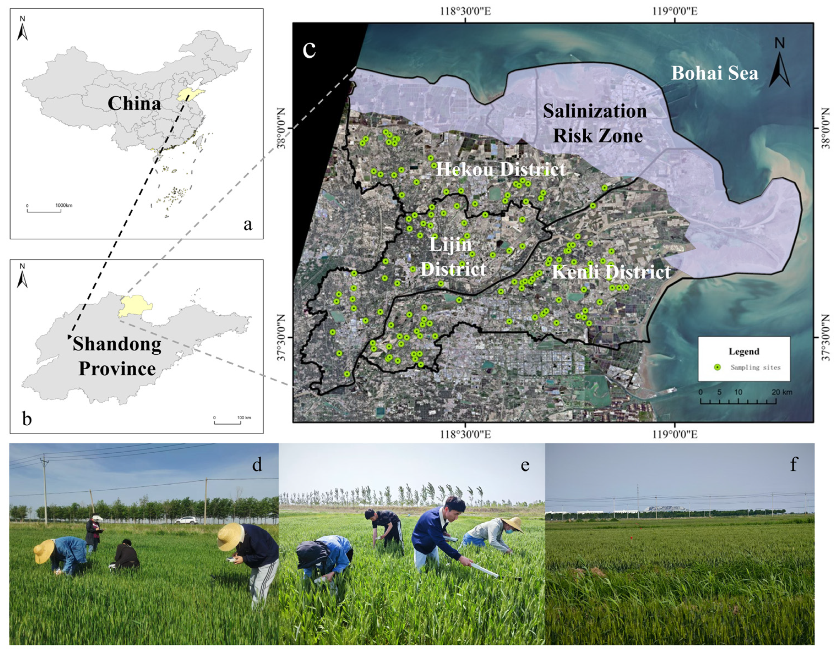
Figure 1. Location of the study area and sampling overview. (a,b) Location of the study area; (c) distribution of sampling points; (d,e) photos taken during sampling; (f) land cover of the study area.
Agronomy 15 01995 g001
Figure 2. Technical flowchart of the study.
Agronomy 15 01995 g002
Figure 3. Correlation between EC and Sentinel-2 MSI band reflectance.
Agronomy 15 01995 g003
Figure 4. Correlation between EC and spectral parameters.
Agronomy 15 01995 g004
Figure 5. Correlation of environmental variables.
Agronomy 15 01995 g005
Figure 6. Performance and improvement of optimal models in four scenarios.
Agronomy 15 01995 g006
Figure 7. Optimal model inversion maps based on spectral parameters (a: Scenario 1, b: Scenario 2, c: Scenario 3, d: Scenario 4).
Agronomy 15 01995 g007
Figure 8. Soil salinity inversion map based on the optimal model.
Agronomy 15 01995 g008
Figure 9. Soil salinity interpolation map based on IDW.
Agronomy 15 01995 g009
Figure 10. Salinity levels and proportions for sample points, inversion, and interpolation results.
Agronomy 15 01995 g010
Figure 11. (a) Correlation coefficients between dominant environmental variables and spectral parameters used in modeling; (b) inter-correlation among dominant environmental variables.
Agronomy 15 01995 g011
Table 1. Source table of environmental variable data.
VariableData Source and ProcessingResolution
PREOpenLandMap (https://openlandmap.org, accessed on 9 September 2023)1000 m
SMField survey data, interpolated using IDW10 m
GELCopernicus DEM30 m
DFSCalculated in ArcGIS from coastline
(coastline from National Earth System Science Data Center)
10 m
SPADField survey data, interpolated using IDW10 m
LAIField survey data, interpolated using IDW10 m
Note: In this study, the resolution was uniformly resampled to 10 m, and PRE represents the average data for the year 2023.
Table 2. Formulas for calculating spectral parameters.
NumberSpectral ParameterFormulaReference
1NDVI B 8 B 4 B 8 + B 4 [39]
2RVI B 8 B 4 [40]
3DVI B 8 B 4 [41]
4EVI 2.5 × B 8 B 4 ( B 8 + 6 B 4 7.5 B 3 + 1 )
5MRESR B 8 B 4 B 5 B 4 [42]
6NREI B 5 B 4 + B 5 + B 8 [43]
7NDVIre B 5 B 8 B 5 + B 8 [44]
8NDVI2 B 8 A B 4 B 8 A + B 4 [45]
9SI1 B 3 × B 4 [46]
10SI2 B 4 2 + B 5 2 + B 6 2
11SI3 B 3 2 + B 4 2
12SI1re B 3 B 5 B 3 + B 5 [19]
13SI2re B 3 × B 5
14S1 B 2 B 4 [47]
15S2 B 2 B 4 B 2 + B 4
Table 3. Descriptive statistics of soil sampling points.
Statistical IndicatorsAll SamplesCalibration SamplesValidation Samples
Quantity1419447
AVG (ms/cm)1.371.391.35
MAX (ms/cm)4.214.213.45
MIN (ms/cm)0.010.010.01
SD (ms/cm)0.800.820.78
CV1.371.391.35
Table 4. Model accuracy based on Scenario 1 (only on spectral parameters).
Statistical
Indicators
Calibration SetValidation Set
R2RMSER2RMSE
MLR0.5730.5300.5670.510
BPNN0.6000.5030.5790.513
RF0.6790.4600.5740.506
SVM0.5940.5170.5740.506
Note: All models passed significance testing at the 0.01 level. The bolded ones represent the optimal model for the current scenario.
Table 5. Model accuracy based on Scenario 2 (spectral parameters in combination with driving variables).
Modeling
Variable
Modeling MethodCalibration SetValidation Set
PerformanceImprovementPerformanceImprovement
R2RMSER2RMSER2RMSER2RMSE
SP + SMMLR0.6460.4650.073−0.0650.6400.5010.073−0.009
BPNN0.6530.4600.053−0.0430.6410.5000.062−0.013
RF0.6960.4300.017−0.030.6530.4920.079−0.014
SVM0.6370.4700.043−0.0470.6010.5270.027\
SP + DFSMLR0.6670.4580.094−0.0720.6560.4820.089−0.028
BPNN0.6230.5080.023\0.6290.4790.05−0.034
RF0.6370.471\\0.6330.5060.059\
SVM0.6670.4680.073−0.0490.6280.4730.054−0.033
SP + SM + DFSMLR0.7430.4230.17−0.1070.7290.4070.162−0.103
BPNN0.6910.4340.091−0.0690.6430.4980.064−0.015
RF0.7230.4110.044−0.0490.6630.4850.089−0.021
SVM0.7710.3880.177−0.1290.6730.4430.099−0.063
Note: “\” indicates no improvement compared to the model without the introduction of environmental variables. All models passed significance testing at the 0.01 level. The bolded ones represent the optimal model for the current scenario.
Table 6. Accuracy of soil salinity inversion models based on Scenario 3 (spectral parameters in combination with response variables).
Modeling
Variable
Modeling MethodCalibration SetValidation Set
PerformanceImprovementPerformanceImprovement
R2RMSER2RMSER2RMSER2RMSE
SP + SPADMLR0.6570.4570.084−0.0730.5780.5420.011\
BPNN0.6850.4380.085−0.0650.5800.5410.001\
RF0.6820.4400.003−0.020.6510.4930.077−0.013
SVM0.6880.4460.094−0.0710.6340.4620.06−0.044
SP + LAIMLR0.6060.5090.033−0.0210.5750.5240.008\
BPNN0.6220.4800.022−0.0230.5680.548\\
RF0.6270.477\\0.6260.5100.052\
SVM0.6540.4770.06−0.040.5440.523\\
SP + SPAD + LAIMLR0.6570.4570.084−0.0730.5740.5450.007\
BPNN0.6600.4870.06−0.0160.6250.4780.046−0.035
RF0.6900.4350.011−0.0250.6560.4900.082−0.016
SVM0.6680.4500.074−0.0670.6450.4970.071−0.009
Note: “\” indicates no improvement compared to the model without the introduction of environmental variables. All models passed significance testing at the 0.01 level. The bolded ones represent the optimal model for the current scenario.
Table 7. Model accuracy based on Scenario 4 (spectral parameters in combination with both driving and response variables).
Modeling
Variable
Modeling ApproachCalibration SetValidation Set
PerformanceImprovementPerformanceImprovement
R2RMSER2RMSER2RMSER2RMSE
SP + SM + SD + SPADMLR0.7780.3680.205−0.1620.7160.4450.149−0.065
BPNN0.7790.3670.179−0.1360.6500.4940.071−0.019
RF0.7500.3900.071−0.070.7030.4550.129−0.051
SVM0.8130.3510.219−0.1660.7220.4090.148−0.097
Note: All models passed significance testing at the 0.01 level. The bolded ones represent the optimal model for the current scenario.
Disclaimer/Publisher’s Note: The statements, opinions and data contained in all publications are solely those of the individual author(s) and contributor(s) and not of MDPI and/or the editor(s). MDPI and/or the editor(s) disclaim responsibility for any injury to people or property resulting from any ideas, methods, instructions or products referred to in the content.