Article

Evapotranspiration Differences, Driving Factors, and Numerical Simulation of Typical Irrigated Wheat Fields in Northwest China

1
Center for Agricultural Water Research in China, China Agricultural University, Beijing 100083, China
2
National Field Scientific Observation and Research Station on Efficient Water Use of Oasis Agriculture in Wuwei, Wuwei 733009, China
3
Key Laboratory of Agricultural Soil and Water Engineering in Arid and Semiarid Areas of the Ministry of Education, Northwest A&F University, Xianyang 712100, China
*
Author to whom correspondence should be addressed.
Agronomy 2025, 15(8), 1984; https://doi.org/10.3390/agronomy15081984
Submission received: 8 June 2025 / Revised: 8 August 2025 / Accepted: 10 August 2025 / Published: 18 August 2025
(This article belongs to the Special Issue Water Saving in Irrigated Agriculture: Series II)

Abstract

Wheat is a staple crop widely sown in Northwest China, and understanding and modelling evapotranspiration (ET) during the wheat-growing stage is important for irrigation scheduling and the efficient use of agricultural water resources. In this study, a four-year observation was conducted on a spring wheat field with border irrigation (BI) treatment and drip irrigation (DI) treatment, based on two Bowen ratio energy balance (BREB) systems. The results showed that the average ET across the whole growing stage scale was 512.0 mm for the BI treatment and 446.9 mm for the DI treatment, and the DI treatment reduced ET by 65.1 mm across the growing stage scale. The driving factors of the changes in ET in the two treatments were investigated using partial correlation analysis after understanding the changing pattern of ET. Net radiation (Rn), soil water content (SWC), and leaf area index (LAI) were the main meteorological, soil, and crop factors leading to the changes in ET in the two treatments. In terms of ET simulation, the SWAP model and different types of machine learning algorithms were used in this study to numerically simulate ET at a daily scale. The total ET values simulated by the SWAP model at the interannual scale were 11.0–14.2% lower than the observed values of ET, and the simulation accuracy varied at different growing stages. In terms of the machine learning simulation of ET, this study is the first to apply five machine learning algorithms to simulate a typical irrigated wheat field in the arid region of Northwest China. It was found that the Stacking algorithm as well as the SWAP model had the optimal simulation among all machine learning algorithms. These findings can provide a scientific basis for irrigation management and the efficient use of agricultural water resources in spring wheat fields in arid regions.

1. Introduction

Evapotranspiration (ET) is an important component of the agricultural water cycle and is the sum of soil evaporation and crop transpiration [1]. Obtaining the values of ET at the field scale and understanding the pattern of its change are important for elucidating the water cycle in the field [2], understanding the water demand during the growing stage of the crop, and formulating accurate irrigation plans [3]. It can be found in the literature that the current methods for obtaining field-scale ET can be classified into the observation and estimation methods. The observational method is to observe the ET using atmospheric instruments, such as the Bowen ratio energy balance (BREB) system and the eddy correlation (EC) system [4,5]. Estimation methods are also important for obtaining ET: for example, researchers use the agricultural water balance method to calculate ET based on the principle of water balance [6]; additionally, the crop coefficient method recommended in the FAO56 [7] is a widely used ET estimation method in global agricultural water management research. In addition to the above two methods, researchers also simulate ET using agricultural hydrological models [8]. At the regional scale, researchers mostly obtain large-scale ET based on remotely sensed data, and a variety of more mature and widely used products are available [9]. The selection of appropriate methods for observing ET from spring wheat fields with typical irrigation practices in the Northwest China arid region is important for the development of reasonable irrigation plans. In addition to obtaining the amount of ET, understanding the driving factors of ET changes is essential for optimizing the management of agricultural water resources and improving the efficiency of water use in the fields. The magnitude of ET is affected by various conditions [10,11], and related studies are crucial for predicting ET in agro-ecosystems in changing environments and ensuring sustainable water use [12]. However, there is a lack of research on the drivers of ET of spring wheat fields at the field-scale in the arid region of Northwest China.
The agricultural hydrological model is a computational procedure that dynamically simulates the growth and development of crops at the field scale under natural environmental conditions [13], and it is an important tool for analyzing the water cycle mechanism in fields and supporting the efficient management of agricultural water resources. The mainstream agricultural hydrological models at present are the AquaCrop model [14], the APSIM model [15], the EPIC model [16], and the SWAP model. The SWAP model (Soil, Water, Air, Plant model) is a common agricultural hydrological model that is widely used in the fields of field hydrology and soil science. The SWAP model compares with the rest of the mainstream agricultural hydrological models by coupling itself with the WOFOST (World Food Studies) model, which can simulate both the hydrological environment of the field and the growth of the crops [17]. Based on the SWAP model, researchers have conducted several studies simulating ET from agricultural fields. Yuan [18] selected an irrigation unit containing field and wasteland in the river-loop irrigation area and studied the water transport between field and wasteland; they found that the SWAP model could better simulate the changes in water flux from fields during the crop-growing stage and the autumn irrigation stage. Li [19] explored the optimal irrigation conditions for spring wheat fields in the Hetao Irrigation District, China, based on the SWAP–WOFOST model. Ma [20] selected three representative sites in the North China Plain, and, based on field experiments and the SWAP model, simulated the water balance parameters of fields, including ET, and determined the optimal irrigation regime for the region. Based on the literature, it can be found that the SWAP model can better simulate the variation in water flux at the field scale; however, there is a lack of relevant studies based on agricultural hydrological models to simulate ET in a typical irrigated spring wheat field in the arid region of Northwest China. Field ET is an important water flux and an essential component of the hydrological processes in fields; therefore, in this study, the SWAP model was used to simulate the variation in ET in two typical irrigated spring wheat fields in the study area.
In addition to the traditional methods of obtaining ET, which mainly rely on physical models or empirical formulas, in recent years, machine learning methods have also been gradually applied in related domains. Compared with the traditional methods, machine learning models, on the whole, involve fewer physical mechanisms in solving problems [21], under which the relationships between different variables and the variables to be predicted can be obtained. Machine learning algorithms have been used to accurately predict and simulate trends in groundwater levels, water storage, and runoff [22,23,24]. The acquisition of ET is also an important area of hydrological research, and researchers have simulated the ET of different ecosystems based on different machine learning algorithms. Before machine learning methods simulate ET, the parameters of the model inputs need to be considered. Compared with the traditional ET calculation models, machine learning models can integrate data from multiple sources, breaking the dependence of traditional methods on a single data source [25]. The data sources of related studies are mostly based on meteorological stations and field observation data at the field scale and remote sensing image data at the regional scale, which have good data migration and scalability. In modelling ET, machine learning has been successfully applied to citrus [26], sugarcane [27], and maize [28,29] fields. Studies in the literature have shown that machine learning studies for ET simulation have been conducted, but they have mainly focused on cash crops such as fruits or maize rather than wheat, a staple crop widely grown in Northwest China. How effective machine learning algorithms are in simulating ET from wheat field with different irrigation methods in the arid region of Northwest China, and how accurate and different the algorithms are from one to another, are subjects that are worthy of study.
Northwest China is a typical inland arid region, where the average annual precipitation is much lower than the average annual evaporation [30]. In order to reduce evaporation and conserve water, most of the fields in the region are covered with plastic film [31], and in addition to mulching, the irrigation methods used in the region are border irrigation and drip irrigation [32]. Wheat is one of the three major staple crops globally and is also the main staple crop grown in this region. During the growing stage of wheat, local farmers need to carry out supplementary irrigation to maintain the normal life activities of the crop, and the large consumption of irrigation water has exacerbated the scarcity of water resources in this region [33]. Therefore, it is of great practical significance to develop reasonable irrigation schedules for spring wheat fields with different irrigation methods in this region and accessing ET during the crop-growing stage also provides a database for developing irrigation schedules. In turn, accurate irrigation plans can be developed to optimize the frequency and volume of irrigation and improve the efficiency of water use in the field. This is of great significance. The main objectives of this study are as follows: (1) We aimed to obtain ET during the growth period of wheat in two typical irrigated fields and explore the main driving factors of ET. (2) We aimed to use the SWAP model to simulate the daily ET of two typical irrigated wheat fields and explore the simulation accuracy of the model. (3) We sought to compare the simulation accuracy and characteristics of the SWAP model and machine learning in simulating ET and select the machine learning algorithm with the best accuracy. In terms of innovation, we integrated four typical machine learning algorithms into the Stacking algorithm to construct an ensemble learning model suitable for predicting ET in spring wheat fields. Additionally, our study was the first in Northwestern China arid region to evaluate the accuracy of the agricultural hydrological model and different types of machine learning algorithms in simulating ET in irrigated wheat fields, providing a certain technical reference for simulating ET in irrigated wheat fields in arid regions.

2. Materials and Methods

2.1. Overview of the Research Area

Field observation experiments were conducted in the mulched wheat field during the growth period from 2017 to 2020 at National Field Scientific Observation and Research Station on Efficient Water Use of Oasis Agriculture in Wuwei of Gansu Province, China (37°87′ N; 102°83′ E). The experimental field has a typical temperate continental climate, with the annual sunshine duration of over 3000 h, average annual temperature about 8 °C, and average accumulated temperature over 3350 °C (>0 °C). It is rich in light and heat resources and suitable for crop growth [34]. Its average annual precipitation is only 164 mm, in contrast with the average annual evaporation of 2000 mm and an average groundwater depth of more than 40 m [35]. During the experiment, we collected soil samples from the 0–100 cm depth range in both the DI treatment and the BI treatment fields prior to wheat sowing using soil auger combined with a core cutter (volume 100 cm3). Each sampling layer was spaced 20 cm apart (0–20 cm, 20–40 cm, 40–60 cm, 60–80 cm, and 80–100 cm), and soil characteristics were determined based on the sample soil. We randomly selected six sampling points in each treatment field. Bulk density was measured using the soil auger-core cutter method, with the specific details presented in [36]. Field capacity was determined using the core cutter method: The core cutters containing the soil samples were covered with filter paper, and were saturated and soaked for 24 h; then, they were placed on air-dried soil for 8 h to drain gravitational water. The soil samples were then dried in a 105 °C oven until constant weight was achieved, obtaining the field capacity. Residual water content was determined as follows: The soil samples were placed in a high-suction centrifuge at 1500 kPa for 24 h. After the free water in the soil was completely removed, it was dried to constant weight using the drying method. The residual water content was calculated based on the mass difference before and after drying. Saturated water content was obtained using the soaking and drying method, with the specific method detailed in [37]. Saturated hydraulic conductivity is determined using the double core cutter head method, with the specific method detailed in the Determination of Forest Soil Moisture and Physical Properties: LY/T 1215-1999 [38]. Soil pH is determined by adding 50 mL of distilled water to different soil samples, centrifuging them, and measuring the pH of the supernatant using the pH meter. Soil salt content was determined by air-drying and grinding the soil samples, passing them through a 1 mm sieve, preparing a soil extract solution with a soil-to-water ratio of 1:5, measuring the conductivity using a conductivity meter [39], and calculating the soil salt content using an empirical formula [40]. The data presented in Table 1 are the average values obtained from different soil samples of the same soil layer in different years. The soil bulk density, field capacity, residual water content, saturated water content, saturated hydraulic conductivity, pH, and soil salt content of the DI (drip irrigation) and BI (border irrigation) of different soil depths are detailed in Table 1.

2.2. Experimental Design

In this study, each experimental field was 50 m × 50 m and was planted with spring wheat (Yongliang 4). The wheat was sown using a seeder, with row spacing of 15 cm for both BI and DI treatments, and sowing density of about 6 × 10⁶ seeds ha−1. To ensure evenly distributed irrigation under BI, a cross-shaped ridge is employed to divide the farmland into four sections (25 m × 25 m each). For DI treatment, the flow rate of the drip heads was 1.38 L h−1, the operating pressure was 0.1 MPa, the row spacing for the drip irrigation belts was 0.6 m, and the spacing between the drip head rows was 0.3 m. Our experiment conditions were identical to those used by local farmers in terms of irrigation schedules, with 10-day irrigation intervals for DI treatment and 20-day intervals for the BI treatment. To prevent wheat lodging, irrigation dates were earlier or later during the experiment period in case of precipitation or windy conditions. The irrigation amount, irrigation date, fertilization amount and fertilization date for wheat from 2017 to 2020 are listed in Table 2.
In the arid agricultural regions of Northwest China, drip irrigation usage can be effective in saving water; we formulated the irrigation activities and amounts in the same way as farmers around the experimental station. The total irrigation amounts in the DI treatment were less than those used in the BI treatment during the growing stage. The average annual fertilization amount in the BI field was 147.0 kg N ha−1, while that in the DI field was 130.1 kg N ha−1.

2.3. Field Observation

An automatic weather station (Hobo, Onset Computer Crop, Rutland, VT, USA) was installed at the experimental station, to obtain meteorological parameters such as precipitation, wind speed, and relative humidity during the growth stage. The weather station is under standard conditions, and the staff at the experimental station regularly irrigate and mow the grass crops on the ground surface of the weather station. ET and radiation flux data during the growing stage were obtained through the Bowen ratio energy balance (BREB) system installed in the BI and DI fields. In this study, both the BI treatment field and DI treatment field were equipped with only one BREB system. The BREB method is based on the energy balance principle proposed by Bowen (1926) [41], which involves measuring the vertical gradients of near-surface air temperature and water vapor pressure to solve for latent heat flux. The core equation is
λ E = R n G 1 + β
where λE is ET expressed in terms of energy, Rn is net radiation, G is soil heat flux density into the ground, and β is the Bowen ratio. β (β = H/λE) is defined as the ratio of H (sensible heat flux) to λE, as shown in the following formula [42]:
β = γ [ T 2 T 1 + Γ ( z 2 z 1 ) ] e 2 e 1
where γ is the pyschrometric parameter, Γ is the adiabatic lapse rate, generally taken as 0.01 °C m−1 for non-saturated air, T2 and e2 are air temperature and water vapor pressure at height z2, and T1 and e1 are air temperature and water vapor pressure at height z1.
Each BREB system consisted of a radiation meter (CNR4, Kipp & Zonen, Delft, The Netherlands), two air temperature and humidity sensors (HMP155, Vaisala, Vantaa, Finland), five soil temperature sensors (109 L, Campbell Scientific, Inc., Logan, UT, USA), five soil water content sensors (CS616, Cambell Scientific, Inc., Logan, UT, USA), two soil heat flux plates (HFP01, Hukseflux, Delft, The Netherlands), and one data logger (CR1000, Campbell Scientific, Inc., Logan, UT, USA). The BREB systems installed in DI and BI field were identical and all in the center of the field. It is worth noting that, as the wheat plants grow, the BREB system adjusted itself to remain 1.5 m above the canopy, without changing its installed position.
Two air temperature and humidity sensors were kept 0.5 m and 1.5 m above the canopy, respectively. The advantage of the BREB system is that it can directly observe ET without requiring wind speed data, meaning that it is suitable for the observation areas ranging from 200 to 100,000 m2 [42]. In this study, the areas of both treatments were 2500 m2, making it appropriate to observe the ET of the two treatments using the BREB system. The weather data and BREB data used in this study have undergone QAQC assessment. During the experimental period, the weather station and BREB system observation instruments were in normal working condition. The grass crop height beneath the meteorological station instruments was stable, and water supply (irrigation and precipitation) was stable and adequate. The installation height of the BREB system instruments and the underlying surface area met the requirements specified in [42]. During the experimental period, weather data were validated through hierarchical testing to ensure data reliability. The QAQC assessment of weather data was conducted by staff from the Chinese National Agricultural Field Observation Research Station (Wuwei, Gansu Province), with the specific principles and workflow detailed in [43]. Data quality assessment for the BREB systems observation were conducted using the methods outlined in [42,44]. During the observation period from 2017 to 2020, an average of 4607 and 4629 datasets were collected annually for the DI treatment and BI treatment, respectively. After screening, 3620 and 3381 datasets were deemed qualified, resulting in data qualification rates of 78.1% and 72.9%, respectively.
The five soil temperature sensors and five soil water content sensors for each treatment were buried at depths of 20 cm, 40 cm, 60 cm, 80 cm, and 100 cm below the soil; the soil temperature sensors (installed in inter-row spacing) and soil water content sensors installed in each treatment were located in the center of each field. The soil heat flux plates were all buried at the depths of 5 cm below the surface. In addition, every 10 days during the spring wheat-growing stage, we took soil samples using the soil auger method at the same depth of the installed soil water content sensors and obtained the soil water content through oven-drying. Specifically, six sample points were randomly located between two rows of drips under the plastic film in the DI treatment, and six sample points in the BI treatment were also located randomly in the soil under the plastic film; the soil water contents obtained by the soil auger method were used to calibrate the data observed by the sensors. Throughout the entire experimental period, the uncalibrated values of soil water content observed by soil water content sensors at different layers under the two treatments were 3.7% to 4.3% higher than those obtained by the soil auger–drying method. All data observed by the soil water content sensors used in this study were calibrated data. In addition, we verified water stress in field during the experiment based on the methods recommended in FAO56:
T A W = 1000 ( θ F C θ W P ) Z r
R A W = p T A W
D r = 1000 ( θ F C θ i ) Z r
K S = 1 , D r R A W
K S = T A W D r ( 1 p ) T A W , D r > R A W
where KS is the coefficient of soil water stress, TAW is the total available soil water in the root zone (mm), θFC is the field capacity (cm3 cm−3), θWP is the wilting point (cm3 cm−3), and Zr is the rooting depth (m), based on the recommendation of the FAO56. Zr is selected to be 0.6 m, 0.8 m, 1.0 m, 1.1 m, and 1.2 m in the seedling stage, jointing stage, heading stage, filling stage, and maturing stage. RAW is the readily available soil water in the root zone (mm), θi is the soil water content in ith day (cm3 cm−3); in our study, we selected the average values of multiple soil layers at the same date, were Dr is the root zone depletion (mm). p is the average fraction of TAW that can be depleted from the root zone before moisture stress occurs, the calculation method is in FAO56. When the KS value is 1, there is no water stress in the field. In this study, the method of obtaining ET based on the BREB system is referred to [45], our method of obtaining ET is scientific and universal. In addition, the accuracy and reliability of the ET obtained in this study based on the BREB system have been verified by [35], so the data quality control and calibration methods are not described in this study. The BREB system was used to accurately obtain the ET of the irrigated wheat fields during the observation period.
Based on the temperature data, we calculated the growing degree days (GDDs) for the two treatments at the growing stage scale using the following formula [46]:
G D D = i = 1 n ( T m a x T m i n 2 T b a s e )
where Tmax and Tmin are the daily maximum and minimum temperature (°C), and Tbase is the base temperature, being 4.5 °C for spring wheat.
During the experimental period, we observed the agronomic traits of DI treatment and BI treatment fields, the main observation indicators including plant height, leaf area index (LAI), and biomass. Specifically, we established six sampling points in each treatment. Every 7–10 days, we randomly selected nine wheat plants with similar growth rates from each sampling point for complete destructive sampling. We measured the plant height of spring wheat during the growing stage using a tape measuring to an accuracy of 0.1 mm. Concurrently, we measured the length and width of all leaves on the aforementioned plants using the same tape and calculated the leaf area index (LAI) based on the method provided by [35]. For biomass acquisition, the plants were divided into four organs: root, stem, leave, and tassel, each placed in different paper bags. After enzyme deactivation, the bags were placed in an oven set at 80 °C and dried for 48 h. The dried samples were then weighed using an electronic scale with a precision of 0.01 g. Based on planting density, the biomass of each organ and total biomass of spring wheat was calculated. This method has been validated by [35]. The experimental layout diagram and on-site photos are shown in Figure 1:
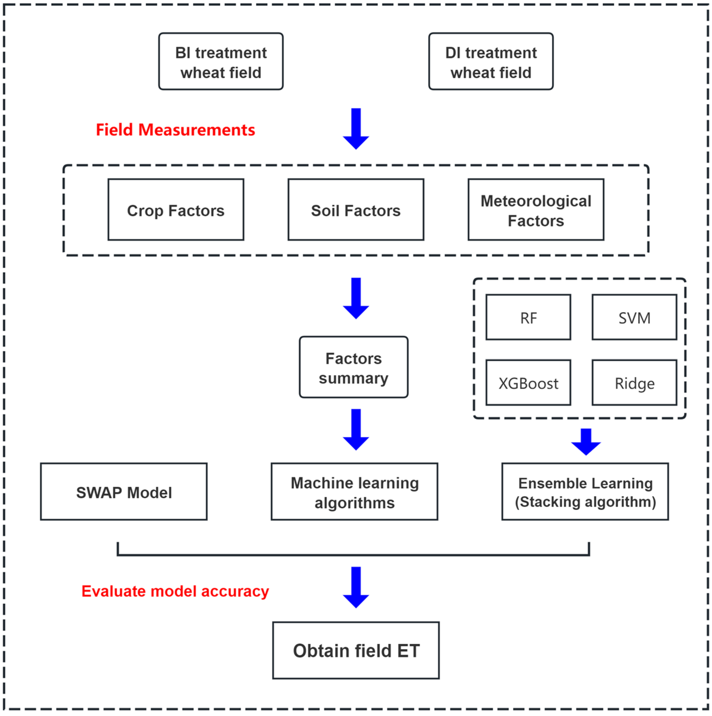
In addition, this study estimating daily ET in spring wheat fields using agricultural hydrological models and machine learning algorithms, as shown in Figure 2. The principles and methods of the different models are described in the Materials and Methods Section.

2.4. Partial Correlation Analysis

Partial correlation analysis was used for assessing the net correlation between two variables after controlling others. It can reveal the true extent of the correlation between two specific variables in the presence of multiple interrelated variables [47]. This study employed this method to determine the relationships among the main driving factors of wheat ET during the observation period. We considered the effects of meteorological, soil, and crop factors on ET, the variables included in the partial correlation analysis primarily encompass the following: crop factors—height (plant height), LAI (leaf area index), and biomass (total biomass including root); soil factors—SWC (soil water content at the depth of 20 cm) and ST (soil temperature at the depth of 20 cm); meteorological factors—Rn (radiation), RH (relative humidity), Ta (air temperature), and WS (wind speed). The formula is as follows:
R ( x y ) = i   =   1 n ( x i x ¯ ) ( y i y ¯ ) i   =   1 n ( x i x ¯ ) 2 i   =   1 n ( y i y ¯ ) 2
R ( i , j h ) = R i j R i h R j h ( 1 R i h 2 ) ( 1 R j h 2 )
where R ( i , j h ) represents the partial correlation coefficient between variable i and j after controlling others. Rij denotes the correlation coefficient between variable i and j, Rih between variable i and h, and Rjh between variable j and h [48].

2.5. SWAP Model

In this study, the SWAP model was adopted to simulate the changes in ET during the growth period in BI fields and DI fields. It was developed by Wageningen University to simulate soil moisture movement, solute transport, heat transfer, and crop growth processes at the field scale. It is a physically based model [49]. Methods provided in the SWAP 4.0 user manual [50] were employed to simulate changes in daily ET during the growth period in BI fields and DI fields. Specifically, the SWAP model in this study simulates ET as follows:
E T = E + T
where ET is crop evapotranspiration (mm d−1), E is soil evaporation (mm d−1), and T is plant transpiration (mm d−1). In the SWAP model, E was simulated as follows:
E p = ( 1.0 V c ) Δ v λ w ( R n G ) + p 1 ρ a i r C a i r λ w ( e s a t e a r a , s o i l ) Δ v + γ a i r ( 1.0 + r s o i l r a , s o i l )
where Ep is the soil evaporation (mm d−1) based on the Penman–Monteith equation; Vc is the canopy cover; Δv is the slope of the vapor pressure curve (kPa °C); λw is the latent heat of vaporization (J kg−1); Rn is the net radiation flux from the surface of the canopy (J m−2 d−1); G is the soil heat flux (J m−2 d−1); p1 represents the unit conversion (86,400 s d−1); ρair is the air density (kg m−3); Cair is the heat capacity of moist air (J kg−1 °C−1); esat is the saturation vapor pressure (kPa); ea is the actual vapor pressure (kPa); ra,soil is the aerodynamic resistance of the soil surface (s m−1); γair is the humidity constant (kPa °C−1); rsoil is the soil resistance of the moist soil (s m−1). In the SWAP model, soil evaporation can also be calculated using Darcy’s law and empirical equations, as follows:
E m a x = k 1 / 2 ( h a t m h 1 z 1 z 1 )
where Emax is the maximum evaporation (mm d−1); k1/2 is the average hydraulic conductivity between the soil surface and adjacent discretized nodes (mm d−1); hatm is the soil hydraulic head in equilibrium with the relative humidity of the air (cm); h1 is the soil hydraulic head at the first node (cm); and z1 is the soil depth at the first node (cm).
E a = β t d r y 1 / 2
where ΣEa is the cumulative actual evaporation (mm); β is a soil-specific parameter characterizing the evaporation process (mm d−1); and tdry is the time (d) after storm rainfall.
E = m i n ( E p , E m a x , E a )
The SWAP model outputs the evaporation from the field as the minimum of Ep, Emax, and ΣEa.
The SWAP model simulates plant transpiration with the following Equation:
T = ( 1 W f r a c ) [ V c v λ w ( R n G ) + p 1 ρ a i r C a i r λ w ( e s a t e a r a i r , c a n ) ] v + γ a i r   [ 1 + r s , m i n r a i r , c a n L A I e f f ]
where T is transpiration (mm d−1); Wfrac is the proportion of canopy wet days; rair,can is the aerodynamic resistance of a uniform crop (s m−1); rs,min is the minimum stomatal resistance (s m−1); LAIeff is the effective leaf area index (cm2 cm−2).
In this study, the irrigation frequency and amounts for both irrigation methods were identical to those used by local farmers for both treatments; after each irrigation, the soil layer from 0 to 100 cm in all treatments reached the soil saturation moisture content. Based on soil water content sensors observation data, it was found that there were no significant differences in SWC between the two treatments during the growing stage. Therefore, in this study, the differences in the simulation process using the SWAP model primarily stemmed from the input of irrigation amounts and frequency, and no modifications were made to the SWAP model itself regarding irrigation method differences. Additionally, both treatments underwent plastic mulching. Considering that mulching primarily affects net radiation and soil temperature, our observation instruments can continuously monitor surface soil temperature and net radiation at high frequencies. Therefore, the input data already reflects the impact of mulching on the field environment.
In simulating the daily-scale ET of the two treatments using the SWAP model, we need to input certain variables and parameters into the model. The variables and parameters input into the model can be divided into two categories. The first category consists of data obtained directly from observations, including meteorological data, crop growth data (leaf area index, plant height, biomass of different organs, etc.), and soil data (soil temperature and soil water content, soil hydraulic parameters). These parameters do not require calibration. The second category of parameters has an important impact on improving the accuracy of model simulations. These parameters cannot be directly observed and obtained. When determining the specific values of these parameters, we need to calibrate them within a certain range. Since we did not change the experimental location during the experimental period and the spring wheat variety sowed was the same, to enhance the applicability of the parameters, we calibrated a set of sensitive parameters and input them into the SWAP model to simulate the daily ET of two treatments in different years. The parameter calibration method in this study referenced the method used in [51], which employs the parameter sensitivity analysis function of the PEST algorithm to identify the model's sensitive parameters, followed by the calibration of these sensitive parameters using the PEST algorithm to obtain optimal parameter values. In terms of model validation, we calibrated the highly sensitive parameters using data from the BI treatment and DI treatment in 2017 and 2018, and validated the model using data from the two treatments in 2019 and 2020. The calibrated parameters are detailed in Table S1 in the Supplementary Materials.

2.6. Machine Learning Algorithms

In the process of simulating the daily ET, considering that ET is influenced by the coupled effects of multiple factors such as soil, crops, and environment, and exhibits nonlinear characteristics, we selected five algorithms based on different principles. These five algorithms are Random Forest (RF), Support Vector Machine (SVM), Extreme Gradient Boosting (XGBoost), Ridge algorithm, and Stacking algorithm. RF algorithms integrate multiple decision trees, reduce model variance through random feature selection, and output ET prediction values based on the nonlinear relationships between input variables using a voting method. SVM algorithms use kernel function mapping to transform different types of variables from a low-dimensional space to a high-dimensional space, construct the optimal regression hyperplane based on the principle of maximizing the margin, and fit ET using high-dimensional feature combinations. XGBoost algorithms integrate multiple decision trees based on the gradient boosting framework, optimize the loss function using Taylor’s second-order expansion, add regularization terms, and establish relationships between different types of input variables and ET. The Ridge algorithm constrains the magnitude of linear regression coefficients through L2 regularization, suppressing multicollinearity interference while preserving the characteristics of input variables, to establish a mapping relationship between ET and input variables. The Stacking algorithm combines the prediction results of multiple models as new features, trains meta-learners to fuse these new features, and simulates ET at the field scale. In summary, the five machine learning algorithms used in this study can be divided into two categories: RF, SVM, XGBoost, and Ridge belong to traditional machine learning algorithms; the Stacking algorithm is an ensemble learning model. Each machine learning algorithm can simulate field-scale ET, but each one’s principles are distinct. Therefore, we selected the aforementioned algorithms for application. A more detailed explanation of the algorithms is provided in the following sections.
Different irrigation methods can lead to differences in the environmental and crop-growing conditions of the two fields. Therefore, we took into account the various variables, such as soil, weather, and crops, when using the machine learning algorithms to simulate ET. Each machine learning algorithm inputs the same type of variables, which include soil data (soil water content at the depth of 20 cm, soil temperature at the depth of 20 cm), plant data (plant height, leaf area index, and total biomass including root), and meteorological data (net radiation, relative humidity, air temperature, and wind speed), and each input parameter is entered in a time step on a daily scale. In this study, we numbered the ET data from the two treatments observed by BREB system and randomly selected 70% of the data (330 of the BI treatment, 323 of the DI treatment) as the training set and the other 30% (142 of the BI treatment, 138 of the DI treatment) as the test set when constructing the estimation model for ET. Each machine learning algorithm was subjected to 5-fold cross-validation. Hyperparameter optimization is crucial for improving prediction accuracy. In our research, we used the ‘caret’ to systematically optimize key hyperparameters for five machine learning algorithms. To ensure the validity of model comparison, all model training and test sets were numbered consistently. Model building and evaluation in this study were implemented through the R language, using the ‘tidyverse’, ‘rio’, ‘caret’, ‘car’, ‘rmisc’, ‘lattice’, ‘metrics’, and ‘magrittr’ packages. The remainder of this section will provide a detailed introduction to the working principles and characteristics of the different algorithms selected for this study. Before introducing the working principles of each algorithm in detail, we intend to reiterate that all types of variables input into the machine learning algorithms have undergone data normalization, and the quality of the input data does not affect the effectiveness of the algorithms in simulating ET. Furthermore, the five algorithms do not interfere with each other in the process of simulating ET.

2.6.1. Random Forest

Random Forest (RF) is a classifier composed of multiple decision trees, which integrate multiple weak classifiers to construct a strong one to improve the accuracy and stability of classification [52,53]. When constructing a Random Forest, it is necessary to extract a certain number of samples from the original data, and then randomly select a certain number of features. Based on these samples and features, a decision tree will be constructed, as will multiple similar decision trees. These decision trees are integrated and classified or regressed through voting methods. The RF algorithm can handle large amounts of data and datasets with high-dimensional features. Since each decision tree in a Random Forest has different samples and features, overfitting can be avoided effectively.

2.6.2. Support Vector Machine

Support Vector Machine (SVM) is a supervised algorithm based on statistical learning theory for classification and regression tasks, and its core mechanism is to map samples into geometric points in a multi-dimensional space by constructing a binary classification linear model in a non-probabilistic form and solving for the optimal hyperplane that maximizes the category interval as a decision boundary [54]. The advantages of this method are reflected in its ability to maintain high classification accuracy in high-dimensional feature spaces and its strong generalization performance for scenarios with a limited number of samples. However, the limitations of the algorithm are that the model is more sensitive to outliers (which may lead to decision surface bias) and the computational efficiency is relatively limited in the face of massive data. Therefore, combining the advantages and disadvantages of this algorithm, we use it as one of the machine learning algorithms for modelling the daily scale of field in this study. For more details, refer to [55].

2.6.3. Extreme Gradient Boosting

The Extreme Gradient Boosting (XGBoost) algorithm is also one of the commonly used methods for solving regression and classification. It iteratively constructs a decision tree model to optimize the loss function and thereby improve performance of the model. It continuously improves the predictive ability of the model with the gradient boosting technology, and controls the complexity of the model leveraging regularization methods to avoid overfitting. It has been successfully applied to predict field ET. For more details, please refer to [56].

2.6.4. Ridge Regression

Ridge regression is a linear model for handling regression problems; on the basis of ordinary least squares regression (OLS), it has introduced regularization terms. By constraining the size of parameters, it can control complexity of the model, thereby preventing overfitting to the data. It can deal with high-degree correlation between features, so that it can stably estimate parameters under acceptable complexity of the model. For more details, please refer to [57].

2.6.5. Stacking

A Stacking algorithm is a type of integration algorithm, which builds and combines different machine learning models to accomplish the learning task. The workflow of the Stacking algorithm in this study is as follows: All sample data from DI treatment and BI treatment were randomly divided into training and testing sets in a 7:3 ratio. Using the training set, prediction models were constructed for RF, SVM, XGBoost, and Ridge, with each machine learning algorithm undergoing five-fold cross-validation. Four-fifths of the training set was used for training in external cross-validation, while one-fifth of the training set was used as the test set for external cross-validation. This process was repeated five times, ensuring that all data in the training set were used as either training or test samples for the models. After completing five-fold cross-validation, each machine learning model generates five sets of prediction results. The prediction results of each machine model for its respective validation set are stacked row-wise to obtain an out-of-sample prediction matrix, and the average prediction value is calculated by averaging these results. The prediction results are then used as input variables to train and validate a second-layer model using multiple linear regression. The second-layer model also employs five-fold cross-validation, ultimately generating four sets of prediction values, which are averaged to obtain the final prediction value. In summary, the Stacking algorithm used in this study first combines different machine learning models into a single learner, then combines them using certain strategies. Its application aims to avoid overfitting the data. For more details on the principles and applications of the Stacking algorithm, refer to [58].

2.7. Statistical Analysis

This study evaluated the simulation effect of different models on ET of BI fields and DI fields with five statistical indicators: coefficient of determination (R2), mean absolute error (MAE), mean bias error (MBE), and root mean square error (RMSE), and percent bias (PBIAS).
R 2 = i = 1 n ( x i x ¯ ) 2 ( y i y ¯ ) 2 i = 1 n ( x i x ¯ ) 2 i = 1 n ( y i y ¯ ) 2
M A E = i = 1 n ( x i y i ) n
M B E = i = 1 n ( x i y i ) n
R M S E = i = 1 n ( x i y i ) 2 n
P B I A S = [ i = 1 n ( y i x i ) i = 1 n y i ] × 100 %
where xi is the predicted value of ET, yi is the observed value of ET, x ¯ is the average value of xi, y ¯ is the average value of yi, and n represents the number of samples.
All variables used in the machine learning algorithms to simulate ET in this study were normalized on an interannual scale using the following formula:
N n o r m = N N m i n N m a x N m i n
where Nmin and Nmax are the minimum value and the maximum value in the original dataset, respectively, and Nnorm is the normalized data.

3. Results

3.1. Dynamics of Meteorological Factors

Table 3 shows meteorological parameters during the growth period of wheat. They were obtained through an automatic meteorological station (Hobo, Onset Computer Crop, Rutland, VT, USA) located 150 m away from the experimental field. Such parameters include wind speed at the height of 2 m above ground (u2), daily maximum temperature (Tmax), daily minimum temperature (Tmin), daily maximum relative humidity (RHmax), daily minimum relative humidity (RHmin), and monthly total precipitation (P). At the interannual scale, except for P, all parameters in the same month have similar values during different years. The variation patterns of Tmax and Tmin are similar, both showing a gradually upward trend and reaching the highest in July, whereas the variation patterns of RHmax and RHmin are different and have a close correlation with P. The total precipitation from 2017 to 2020 was 76.6 mm, 41.4 mm, 110.2 mm, and 57.6 mm, respectively.

3.2. Changes in ET in Wheat Fields

This study investigated the ET of a spring wheat field under DI and BI treatments at the growing stage scale. The division of each growing stage and growing degree days (GDD) are shown in Table 4.
Table 4 shows different growing stages for BI and DI fields during the experimental period. Although the sowing date is the same, the growth period under the DI treatment is shortened by 6 days In comparison with the BI treatment. Except for the seedling period, the average length of each growth period under the DI treatment is shorter than that under the BI treatment. Figure 3 shows the dynamics of SWC at different soil layers under BI treatment and DI treatment during the experimental period. Before showing the dynamics of SWC, we calculated the coefficient of soil water stress (KS) at the growing stage scale. For both treatments, KS was 1 at different growing stages and in different years, indicating no water stress. Figure 3a–h show the dynamics of SWC at different soil layers for the two treatments. As shown in the figures, within a complete growing stage (from seedling stage to maturing stage), the dynamics of SWC changes were similar across different soil layers. With water input (irrigation and precipitation), SWC exhibited a phased increase–decrease trend. Additionally, the shallow soil layer (0−20 cm) exhibits the largest fluctuations in SWC, with deeper soil layers showing smaller fluctuations in SWC. Figure 3i shows a comparison of the average SWC values at different growing stages for the two treatments. The SWC data in Figure 3i are the average values of SWC data from different soil layers on the same day. As shown in Figure 3i, except for the maturing stage, there were significant differences in the average SWC values between the two treatments at other growing stages. The lack of significant differences in SWC between the two treatments during the maturing stage may be related to the low water input in both treatments in this growing stage.
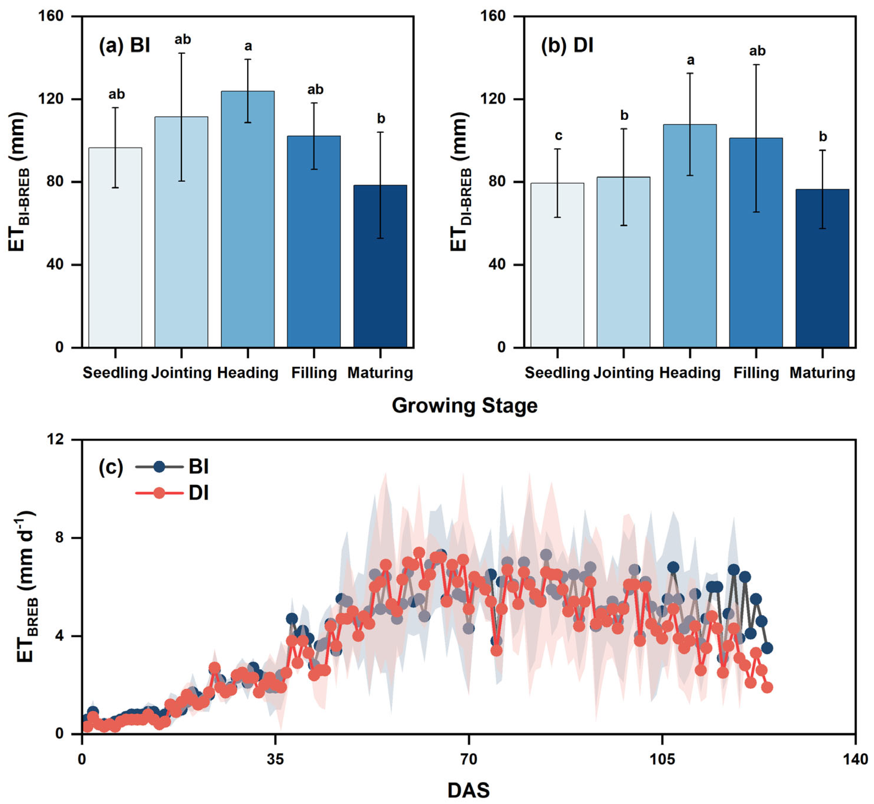
Based on the BREB system, we observed the ETBREB of the BI treatment and DI treatment during the whole growing stage from 2017 to 2020, Figure 4 shows the ETBREB of the two treatments at the growing stage scale and daily scale. Figure 4a shows the average ETBREB of the BI treatment at different growing stages, which were 96.5 mm, 111.3 mm, 123.9 mm, 102.1 mm, and 78.4 mm from seedlings to the maturing stage. Figure 4b shows the average ETBREB of DI treatment at different growing stages, which were 79.4 mm, 82.3 mm, 107.7 mm, 101.1 mm, and 76.4 mm from seedling stage to maturity stage. It can be found that the ETBREB of BI treatment was higher than the DI treatment at all growing stages, and the ETBREB of DI treatment was 65.3 mm lower than the BI treatment at the whole growing stage. The lower ET observed with DI treatment compared to BI treatment during the growing stage can be explained from two perspectives. From the perspective of water balance, DI treatment results in lower water input throughout the whole growing stage, thereby reducing total water consumption. From the perspective of irrigation methods and water input, the DI treatment compared to the BI treatment, has the characteristic of frequent, small amount irrigation. Irrigation water is directly delivered to the crop surroundings through drip irrigation pipes, reducing soil evaporation compared to the BI treatment and thereby lowering ET during the growing stage. In summary, based on this study, it can be observed that DI treatment has lower irrigation amounts and ET at the growing stage scale. The adoption of drip irrigation in this region demonstrates water-saving benefits. In our experiment, the DI treatment had lower ET with less irrigation, and the use of drip irrigation in this area has a certain water saving benefit. Figure 4c shows the daily scale changes in ETBREB during the growing stage of spring wheat in both treatments, the two treatments had the same change pattern, which showed an increasing and then decreasing trend, and the daily ETBREB of spring wheat in both treatments reached the peak value from 60 days to 90 days after sowing. The average daily ETBREB values for the BI treatment of spring wheat in the seedling stage, the jointing stage, the heading stage, the filling stage, and the maturing stage were 2.1 mm d−1, 6.2 mm d−1, 6.4 mm d−1, 5.4 mm d−1, and 4.1 mm d−1, and the average daily ETBREB for the whole growing stage was 4.2 mm d−1. The average daily ETBREB values for the DI treatment of the spring wheat in the seedling stage, the jointing stage, the heading stage, the filling stage, and the maturing stage were 1.4 mm d−1, 6.2 mm d−1, 6.1 mm d−1, 5.3 mm d−1, and 4.3 mm d−1, and the average daily ETBREB for the whole growing stage was 3.8 mm d−1. From the heading stage to maturing stage, both the total ET and daily average ET of the BI treatment and DI treatment showed a gradual decreasing trend, which may be related to the growth condition of spring wheat. We analyzed the changes in leaf area index (LAI) of spring wheat under the two treatments during the experimental period (Figure S2) and found that LAI gradually decreased from the heading stage. The decrease in LAI led to a decrease in transpiration at the growing stage, which in turn resulted in a decrease in ET.

3.3. Driving Factors of ET in Wheat Fields

This study used partial correlation analysis to determine the driving factors of ET during the growing stage. These variables are identical to those input into the machine learning algorithms: crop factors—height (plant height), LAI (leaf area index), and biomass (total biomass including root); soil factors—SWC (soil water content at the depth of 20 cm) and ST (soil temperature at the depth of 20 cm); meteorological factors—Rn (net radiation), RH (relative humidity), Ta (air temperature), and WS (wind speed). Figure 5 shows the correlations of the main driving factors for the BI treatment (Figure 5a) and the DI treatment (Figure 5b). For both the BI treatment and the DI treatment, Rn was the most significant driving factor of ET. In terms of crop factors, biomass and LAI had a significant influence on ET for both treatments (p < 0.01). In terms of soil factors, SWC had a significant influence of ET for both treatments (p < 0.01). For treatments, both the types of variables significantly affecting ET are largely the same, but various partial correlation coefficients differ. Additionally, ST and RH have little effects on ET under both treatments.

3.4. ET Simulation with the SWAP Model

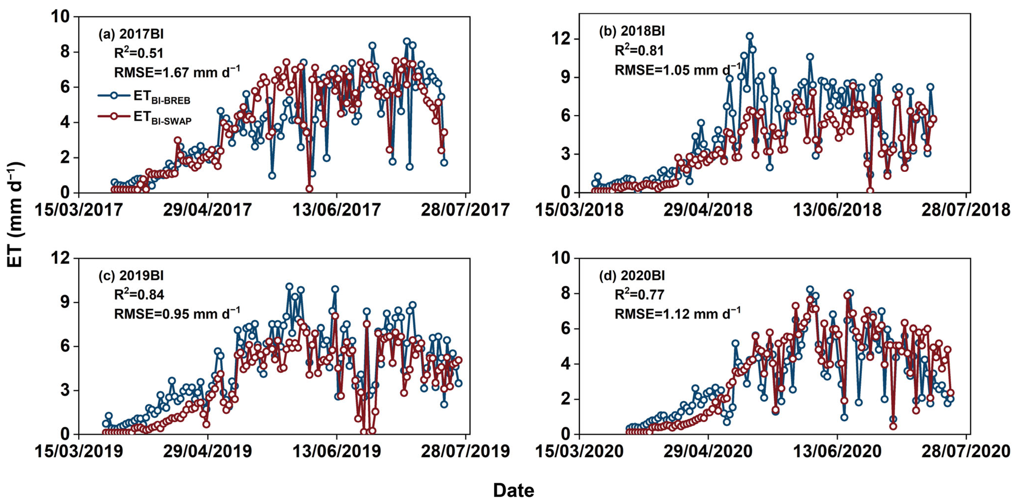
Based on the SWAP model, changes in ET during the growth period of wheat under two irrigation methods were simulated as shown in Figure 6 and Figure 7. The red lines represent the wheat field ET simulated by the SWAP model (ETSWAP), while the blue ones observed by the BREB system (ETBREB). Figure 6a–d represent changes in ET of wheat fields under the BI treatment from 2017 to 2020. ETSWAP and ETBREB during the four-year experimental period showed similar fluctuations. The simulation accuracy varied in different years. At the interannual scale, the mean bias error (MBE) between ETBISWAP and ETBIBREB varies from −1.05 mm d−1 to 0.29 mm d−1. As for the percent bias (PBIAS), it varied between −8.8% and 22.6% at the interannual scale, with the PBIAS of 14.2% during the 2017−2020 experimental period. Based on the results of this study, the SWAP model underestimated ET by 14.2% compared with ETBREB.
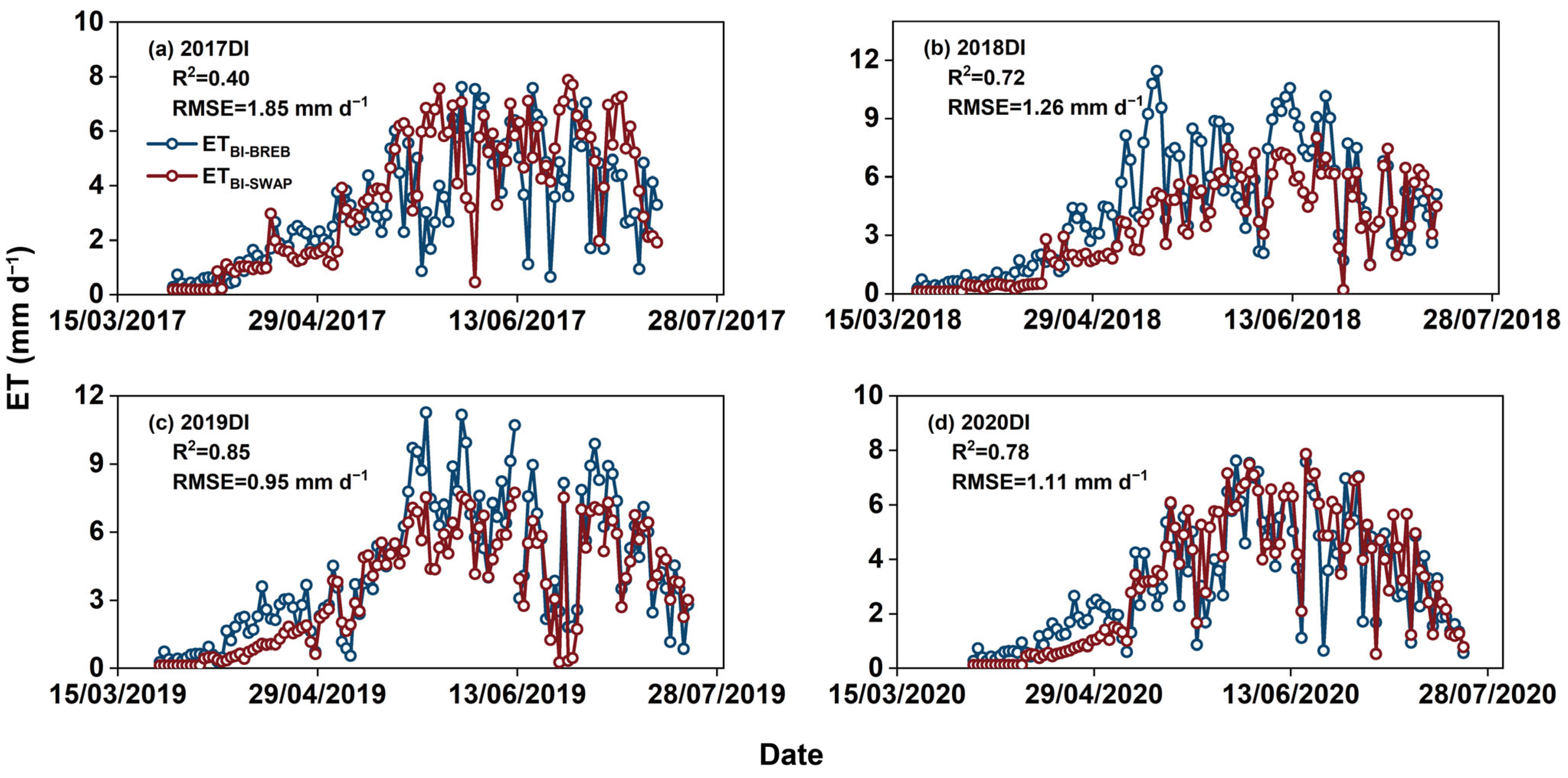
Figure 7a–d represent the changes in ET in wheat fields under the DI treatment from 2017 to 2020. ETSWAP and ETBREB during the four-year experimental period showed similar fluctuations. The simulation accuracy varied in different years as well. At the interannual scale, the MBE between ETDISWAP and ETDIBREB varies from −1.06 mm d−1 to 0.11 mm d−1. As for the PBIAS, it varied between −2.3% and 23.9% at the interannual scale, with a PBIAS of 11.0% during the 2017–2020 experimental period. Based on the results of this study, the SWAP model underestimated ET by 11.0% compared with ETBREB.
Table 5 shows the values of ETSWAP and ETBREB at different growing stages under DI treatment and BI treatment; it can be observed that the SWAP model performs better in simulating ET under BI treatment and DI treatment in 2017 and 2020 compared to 2018 and 2019. This may be attributable to two factors. In terms of water input (P + I), the water input in DI treatment and BI treatment was higher in 2018 and 2019 than in 2017 and 2020. The higher water input indirectly led to greater water consumption. However, the SWAP model performed less effectively in capturing changes in ET following water input in May 2018 and May 2019 for both treatments. Secondly, based on the findings from Section 3.3, Rn is the primary positive driver of ET changes in BI treatment and DI treatment. We analyzed the Rn for BI treatment and DI treatment across different years and found that the average Rn values for 2018 and 2019 spring wheat’s whole growing stage were 6.8% higher (BI treatment) and 9.2% higher (DI treatment) than those for 2017 and 2020. The changes in ET caused by differences in Rn may not have been fully captured by the SWAP model.

3.5. ET Simulation with Machine Learning Algorithms

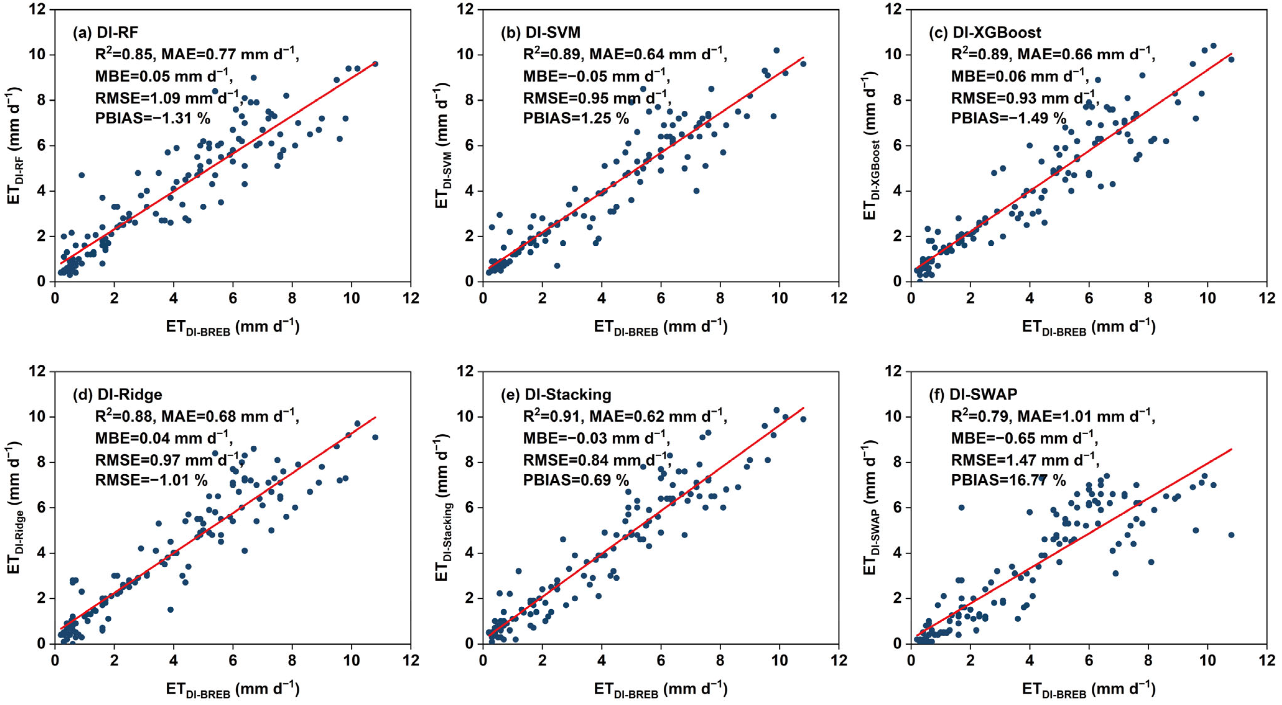
To compare the simulation accuracy of the SWAP model and machine learning algorithms, we applied five machine learning algorithms to simulate the daily ET of wheat fields under both the BI treatment and the DI treatment during the experimental period. Figure 8 shows the scatter plots of ET of wheat fields under the BI treatment simulated by the five algorithms and the SWAP model. Figure 8a–f show the daily ET simulation results of RF, SVM, XGBoost, Ridge, Stacking, and the SWAP model, respectively. Since the machine learning algorithms selected 70% of the training sets for the entire growth period under the BI treatment and the DI treatment, the scatter plots were compared with 30% of the remaining data in the SWAP model. In Figure 8f, the ETBI-SWAP data were selected at the same time as those in Figure 8a–e. It can be observed that R2 and RMSE values of the five machine learning algorithms are higher than those of the SWAP model (R2 = 0.74, RMSE = 1.50 mm d−1). The Stacking algorithm has the highest calculated R2 of 0.83, and the Stacking algorithm also has the lowest calculated RMSE of 1.13 mm d−1. In addition, we analyzed the effectiveness of different methods of simulating ET based on MBE and PBIAS. The MBE of different machine learning algorithms in BI treatment varied from −0.07 mm d−1 to 0.12 mm d−1, while MBEBISWAP was −0.61 mm d−1. In terms of PBIAS, the SWAP model's performance in simulating ET (PBIASBISWAP = 14.99%) was weaker than that of the various machine learning algorithms (−3.0% to 1.7%).
Figure 9a–f show the simulation results of the RF, SVM, XGBoost, Ridge, and Stacking machine learning algorithms and the SWAP model. The vertical axis represents the daily ET under the DI treatment obtained with various simulation methods, while the horizontal axis is ETBREB. Among the five machine learning algorithms, the Stacking algorithm had the highest R2 at 0.91, while the RF algorithm had the lowest R2 at 0.85. The Stacking algorithm generated the highest R2 and the lowest RMSE of 0.84 mm d−1. It thus can be seen that the SWAP model had poorer performance in simulating ET under the DI treatment than the five machine learning algorithms, with an R2 of 0.79 and an RMSE of 1.47 mm d−1. In terms of MBE, the values of different machine learning algorithms vary between −0.03 mm d−1 and 0.06 mm d−1, all better than the SWAP model (MBEDISWAP = −0.65 mm d−1). In terms of the PBIAS, overall, the Stacking algorithm performed the best, with PBIASDIStacking at 0.69%, while the SWAP model performed poorly, with PBIASDISWAP at 16.77%. Combining the results of Figure 8 and Figure 9, we can observe that for both treatments in our study, the SWAP model in this study performed poorly compared to the machine learning algorithms in terms of simulation accuracy. Additionally, the Stacking algorithm performed best in simulating ET for both treatments, with superior values across multiple statistical metrics compared to the other machine learning algorithms and the SWAP model.

4. Discussions

4.1. ET of the Field

ET is one of the important components of the field water cycle and the focus of research on field hydrological processes, and understanding field ET is of great significance for irrigation planning. It is of practical value and scientific significance to observe different types of typical irrigated fields in different years by means of high-precision and high-frequency observation instruments. Northwest China is a major agricultural production area, and wheat is the main staple crop grown in the region. The precipitation during the growing stage of wheat is much less than the ET, so supplementary irrigation is needed during agricultural production. In this study, the average ET during the growing stage of spring wheat in DI treatment was 446.9 mm and in BI treatment was 512.0 mm, the shift in irrigation reduced the ET at the growing stage scale of wheat, which is consistent with the findings of [59]. Specifically, DI treatment has lower ET at the growing stage scale, which can be explained from the following perspectives. In terms of irrigation amount, the DI treatment in this study involved less irrigation than the BI treatment at the growing stage scale, and the water input term (irrigation and precipitation) of the DI treatment was smaller than that of the BI treatment during the crop’s growing stage, so the ET of the DI treatment was smaller than that of the BI treatment. In terms of soil evaporation (E), since E is higher than precipitation in field in the arid region of Northwest China [60], most of the field in this region is treated with mulching, and therefore only the effect of the change in irrigation on ET caused by the change in irrigation method was explored in this study. In the region where this study was conducted, most of the farmers in the region engage in irrigation characterized by small amounts and multiple instances, using drip irrigation equipment; the DI treatment has a smaller amount in a single irrigation than the BI treatment and the wetting front of the DI treatment is different from that of the BI treatment, which reduces E from the field [61], which reduces the ineffective loss of water from the field. Comparing and analyzing the differences between the spring wheat-growing stage scale ET in this study and the rest of the ET in the region can provide data support for field-scale studies for the optimization study of regional crop cropping systems. Our results showed that the ET during the growing stage of wheat was lower than that of maize under the same irrigation conditions compared with other typical crop crops grown in Northwest China [62]. During the growing stage of spring wheat in this study, ET was relatively low compared to the rest of the staple crops, but higher than that of cash crops such as cabbage [30] and cotton [63] grown in the region. Overall, this study systematically obtained high-frequency and high-precision ET from field with different irrigation methods in the arid region through the BREB system, which provided a large amount of data for subsequent studies.

4.2. Analysis of Driving Factors for Field ET

It is important to research the drivers of ET in order to understand the mechanisms of ET changes in the field and to formulate reasonable irrigation policies. Based on the literature study, it can be found that most of the previous studies focused on maize [64], grassland [65], or regional-scale crop-rotation fields [66], rather than the drivers of ET in irrigated spring wheat field. Among the existing studies on the drivers of field ET, only a few drivers were included. In this study, LAI and Biomass were considered in terms of crop factors, and Rn, SWC, ST, Ta, and RH were considered in terms of environmental factors, which comprehensively illustrated the effects of crop and environmental factors on the variation in ET in wheat fields. The results of the study showed that Rn was the main environmental factor during the growing stage of the two irrigated wheat fields, which can be explained from the following perspectives. Radiation is the direct source of energy for the ET process; net radiation provides the latent heat of vaporization for soil evaporation and crop transpiration, and ET is limited by radiation mainly when soil moisture is sufficient in the field. In terms of pathways, radiation fluxes are transported to the field surface as well as to the crop canopy, which in turn increases leaf and soil temperatures and affects field ET. The finding that radiation, as a major driver of ET in spring wheat, is essentially a result of synergistic effects of energy supply, physiological responses, and environmental feedback is similar to the findings evidenced by the results of a study conducted in a maize field [31]. In addition, SWC and LAI were also the main drivers of ET in irrigated wheat fields for both treatments, reflecting the drivers of ET by soil moisture and the crop's own growth conditions, respectively. For the irrigated spring wheat field in this study, although the irrigation method changed the total ET during the growing stage, the driver of ET did not change with the shift of the irrigation method, and the finding of this result also provides a theoretical basis for the subsequent optimization of the irrigation regimes for typical spring wheat field in arid regions.

4.3. Evaluation of Simulation ET Accuracy in Different Methods

In this study, we compared the accuracy of the SWAP model and machine learning in simulating ET from wheat fields under the BI and DI treatments. The results showed that the simulation accuracy of the SWAP model fluctuated greatly in different years. ETBI-SWAP was 14.2% lower than ETBI-BREB during wheat-growing stage, and the simulation accuracy of the SWAP model was better in assessing the DI treatment than the BI treatment, ETDI-SWAP was 11.0% lower than ETDI-BREB. The SWAP model had the highest accuracy in simulating ET at the maturity stage (BI treatment and DI treatment), while the SWAP model had the lowest simulation accuracy at the seedling stage and jointing stage (BI treatment and DI treatment). ETSWAP underestimated ET in irrigated wheat fields during the growing stage due to the low simulation accuracy of the SWAP model at the seedling stage and jointing stages. Combining the simulation accuracy of the SWAP model and different types of machine learning algorithms during the experimental period, it can be found that the machine learning algorithms have higher simulation accuracy of ET than the SWAP model. These results can be explained in the following aspects: the SWAP model is mainly constructed based on the energy balance and water transport equations when simulating ET, which requires preset parameters and simplified assumptions, whereas ET is affected by the dynamic coupling of meteorological, soil, and physiological factors of the crop, which has a strong nonlinear effect [67]. Machine learning algorithms can capture the nonlinear interactions between different variables; in addition, machine learning models have obvious advantages over agricultural hydrological models in terms of rate-setting parameters. Some previous studies on machine learning for ET simulation [68,69] concluded that machine learning has good simulation accuracy. In addition, from the evaluated statistical indicators, the five machine learning algorithms had higher R2 and lower RMSE than the SWAP model for the BI treatment and the DI treatment, and there was no significant overestimation or underestimation in different years and different growing stages, which corroborated the above opinion. Among the five machine learning algorithms applied in this study, the Stacking algorithm is optimal in modelling both processing ET, which uses the previous four algorithms as a basic model, integrating the advantages of multiple basic models; this, in turn, improves the algorithm's accuracy and robustness. The machine learning algorithms produced good simulation accuracy in both BI and DI treatments during the experiment, filling a research gap in the use of machine learning algorithms to simulate ET in irrigated wheat fields in Northwest China.

4.4. Advantages and Disadvantages of Different Methods for Obtaining ET

Obtaining field ET is of great significance for understanding hydrological processes of the agroecosystem and formulating reasonable irrigation plans and is a direction widely studied by researchers [70]. At the field scale, many researchers use the water balance method based on soil water content [71]. This method takes into account many factors in the hydrological process, but can only obtain periodic ET, generally at high time intervals. The KC-ET0 method is based on KC of a specific crop combined with ET0, which can obtain daily ET [72,73]. However, this method is based on the estimated KC, so that the obtained ET is an estimated value rather than a true one. In addition, although direct observation methods such as the EC system and the BREB system have higher measurement accuracy, they are expensive in both production and installation and have demanding observation surface requirements but limited observation range, which therefore has restricted their promotion on a large scale [74,75]. The remote sensing method can obtain large-scale ET data, but due to limitations in pixel size, satellite transit frequency, and data accuracy, it is currently difficult to obtain ET in a timely manner at the field scale [76]. In this study, the crop model method (SWAP model) and five machine learning algorithms were employed to obtain ET of wheat fields under two irrigation methods. In terms of ET simulation accuracy, the crop model had a good effect on the whole, but tended to underestimate data. Unlike traditional ET estimation methods, machine learning algorithms do not need a large number of data types and samples. Different machine learning algorithms construct different complex models, which has improved ET simulation accuracy and overcome limitations of traditional methods. Subsequent research should focus on increasing the interpretability of machine learning algorithms. The machine learning algorithms used in this study can guide actual irrigation scheduling at the field scale. Researchers can obtain dynamic changes in SWC based on soil moisture sensors and combine them with ET obtained from machine learning algorithms to construct a probabilistic framework for irrigation requirements [77], which is also the direction for subsequent research. In addition, future research should also improve the interpretability of machine learning algorithms for ET simulation results.

4.5. The Feasibility of Applying ET Simulation with Machine Learning in Practice

This study is the first to apply machine learning algorithms to simulate the daily ET of irrigated wheat fields in Northwest China, and has achieved high simulation accuracy. It has been proven that simulating field daily ET through machine learning algorithms is feasible. With gradual application of machine learning methods in hydrology [78], their footprints have gradually expanded from academic research to field applications. This study is based on meteorological data, soil data, and crop data, which can be used to simulate high-precision field daily ET, which is particularly important for the efficient management of agricultural water resources. Although the existing studies have shown that crop models can be nested into irrigation decision systems to guide irrigation [79], this study shows that the crop model requires a large number of parameters and cannot obtain optimal simulation results when simulating certain growth periods. This study has employed five machine learning algorithms to simulate daily ET. Subsequently, irrigation optimization can be carried out at the field scale by combining the precipitation and irrigation amount from the previous stage. It is a more accurate irrigation optimization method that can be developed utilizing the existing field observation instruments. Previous studies have also shown that machine learning methods have broad application prospects in supporting irrigation decisions [80,81]. This study has explored the feasibility of machine learning methods in simulating ET of typical irrigated wheat field in Northwest China. The research results show that they can accurately simulate ET of wheat fields in Northwest China, providing more accurate and efficient irrigation management solutions for subsequent researchers. It is worth noting that we have conducted multi-year studies on a field scale. The experimental station where this research was located is a national-level research platform. The wheat variety sowed was widely cultivated in the region, and the agronomic practices and irrigation methods employed were identical to those used by local farmers. Therefore, this study accurately represents the actual level of wheat cultivation in the region where the research was located and is thus representative. Due to various factors such as labor power and economic constraints, this study was conducted at the field scale but not at other sites, which is a limitation of this study. However, the multi-year field experiments partially compensate for this limitation in terms of temporal scale. Our study provides a large amount of field observation data for subsequent research and validates the feasibility of obtaining the ET of spring wheat under different irrigation methods in Northwest China using various methods. Subsequent research could consider applying the algorithms and methods used in this study to obtain ET to studies of similar crops. To enhance the research scale and applicability, future studies could integrate remote sensing imagery data into the machine learning algorithms used in this study to obtain regional-scale ET.

5. Conclusions

This study conducted a four-year observational experiment in typical irrigated spring wheat fields in the arid region of Northwest China, systematically investigating the patterns of evapotranspiration (ET) and its primary driving factors under different irrigation methods (drip irrigation, DI, and border irrigation, BI), and simulating ET using various methods. The main conclusions are as follows: The change in irrigation method (from border irrigation to drip irrigation) reduced ET of spring wheat fields, with an average decrease of 65.1 mm during the growing stage scale. Net radiation (Rn), soil water content (SWC), and leaf area index (LAI) were the main meteorological, soil, and crop factors contributing to the changes in ET. In terms of ET simulation, the SWAP model in this study can reflect the trend of ET changes at the growing stage scale, with an underestimation range of 11.0% to 14.2%. In addition to the SWAP model, this study employed various machine learning algorithms to simulate ET. Among them, the Stacking ensemble learning model, which was first applied to a spring wheat field in the arid regions of Northwest China, demonstrated the best simulation performance. The aforementioned research provides a theoretical basis for simulating the ET of irrigated fields in arid regions, and the findings can serve as an important reference for the efficient management of agricultural water resources in spring wheat cultivation in Northwest China.

Supplementary Materials

The following supporting information can be downloaded at: https://www.mdpi.com/article/10.3390/agronomy15081984/s1, Figure S1: Changes in plant height during the growing period of wheat under drip irrigation (DI) and border irrigation (BI); Figure S2: The variation pattern of leaf area index (LAI) during the growth period of wheat under two irrigation methods (DI and BI); Figure S3: Comparison of above-ground biomass during wheat harvest between two irrigation methods (DI and BI); Figure S4: Comparison of wheat yield between two irrigation methods (DI and BI); Figure S5: Comparison of wheat Harvest Index between two irrigation methods (DI and BI); Table S1: Calibrated parameters for SWAP model inputs; Table S2: The average temperature of different soil layers in different growing stages of wheat fields under two irrigation methods.

Author Contributions

Conceptualization, T.Y., H.C., and H.Y.; methodology, T.Y. and H.Y.; software, T.Y. and H.C.; validation, S.L.; data curation, D.Y.; writing—original draft preparation, T.Y.; writing—review and editing, H.C. and S.L.; visualization, Z.L. and D.Y.; supervision, S.L.; project administration, S.L.; funding acquisition, S.L. All authors have read and agreed to the published version of the manuscript.

Funding

This research was supported by the Central Government Guidance Fund for Local Science and Technology Development Projects (Grant No.23ZYQH0298).

Data Availability Statement

Data will be made available on request.

Conflicts of Interest

The authors declare no conflicts of interest.

References

  1. Jiang, X.M.; Wang, Y.T.; A, Y.L.; Wang, G.Q.; Zhang, X.J.; Ma, G.W.; Duan, L.M.; Liu, K. Optimizing actual evapotranspiration simulation to identify evapotranspiration partitioning variations: A fusion of physical processes and machine learning techniques. Agric. Water Manag. 2024, 295, 108755. [Google Scholar] [CrossRef]
  2. Li, M.; Chu, R.H.; Abu, R.M.; Towfiqul, T.; Jiang, Y.L.; Shen, S.H. Estimating daily actual evapotranspiration of a rice-wheat rotation system in typical farmland in the Huai River Basin using a two-step model and two one-step models. J. Integr. Agric. 2021, 20, 274–288. [Google Scholar] [CrossRef]
  3. Wang, B.; Dam, J.v.; Yang, X.L.; Coen, R.; Du, T.S.; Kang, S.Z. Reducing water productivity gap by optimizing irrigation regime for winter wheat-summer maize system in the North China Plain. Agric. Water Manag. 2023, 280, 108229. [Google Scholar] [CrossRef]
  4. Xiong, Y.J.; Chen, X.H.; Tang, L.; Wang, H. Comparison of surface renewal and Bowen ratio derived evapotranspiration measurements in an arid vineyard. J. Hydrol. 2022, 613, 128474. [Google Scholar] [CrossRef]
  5. Bian, J.; Hu, X.L.; Shi, L.S.; Min, L.L.; Zhang, Y.C.; Shen, Y.J.; Zhao, F.H.; Zha, Y.Y.; Lian, X.; Huang, J.S. Improving the evapotranspiration estimation by considering the effect of flux footprint climatology. J. Hydrol. 2024, 631, 130769. [Google Scholar] [CrossRef]
  6. Li, H.T.; Shao, L.W.; Liu, X.W.; Sun, H.Y.; Chen, S.Y.; Zhang, X.Y. What matters more, biomass accumulation or allocation, in yield and water productivity improvement for winter wheat during the past two decades? Eur. J. Agron. 2023, 149, 126910. [Google Scholar] [CrossRef]
  7. Allen, R.G.; Pereira, L.S.; Raes, D.; Smith, M. Crop Evapotranspiration-Guidelines for Computing Crop Water Requirements; FAO Irrigation and Drainage Paper No.56; FAO: Rome, Italy, 1998. [Google Scholar]
  8. Li, P.; Ren, L. Evaluating the differences in irrigation methods for winter wheat under limited irrigation quotas in the water-food-economy nexus in the North China Plain. Agric. Water Manag. 2023, 289, 108497. [Google Scholar] [CrossRef]
  9. Amani, S.; Hossein, S.M. A review of machine learning models and influential factors for estimating evapotranspiration using remote sensing and ground-based data. Agric. Water Manag. 2023, 284, 108324. [Google Scholar] [CrossRef]
  10. Wang, F.J.; Liang, W.; Fu, B.J.; Jin, Z.; Yan, J.W.; Zhang, W.B.; Fu, S.Y.; Yan, N.N. Changes of cropland evapotranspiration and its driving factors on the loess plateau of China. Sci. Total Environ. 2020, 728, 138582. [Google Scholar] [CrossRef] [PubMed]
  11. Li, X.L.; Xu, X.F.; Tian, W.; Tian, J.; He, C.S. Contribution of climate change and vegetation restoration to interannual variability of evapotranspiration in the agro-pastoral ecotone in northern China. Ecol. Indic. 2023, 154, 110485. [Google Scholar] [CrossRef]
  12. Chen, Y.M.; Xue, Y.J.; Hu, Y.M. How multiple factors control evapotranspiration in North America evergreen needleleaf forests. Sci. Total Environ. 2018, 622, 1217–1224. [Google Scholar] [CrossRef]
  13. Zhang, Z.T.; Sun, S.; Zhang, F.L.; Guo, S.B.; Guo, E.J.; Loi, Z.J.; Zhao, J.; Zhao, C.; Li, T.; Yang, X.G. Using estimated radiation in crop models amplified the negative impacts of climate variability on maize and winter wheat yields in China. Agric. For. Meteorol. 2022, 318, 108914. [Google Scholar] [CrossRef]
  14. He, Q.S.; Li, S.E.; Hu, D.; Wang, Y.H.; Cong, X. Performance assessment of the AquaCrop model for film-mulched maize with full drip irrigation in Northwest China. Irrig. Sci. 2021, 39, 277–292. [Google Scholar] [CrossRef]
  15. Yan, Z.Z.; Zhang, X.Y.; Rashid, M.A.; Li, H.J.; Jing, H.C.; Hochman, Z. Assessment of the sustainability of different cropping systems under three irrigation strategies in the North China Plain under climate change. Agric. Syst. 2020, 178, 102745. [Google Scholar] [CrossRef]
  16. Yang, J.H.; Wu, J.J.; Liu, L.Z.; Zhou, H.K.; Gong, A.D.; Han, X.Y.; Zhao, W.H. Responses of winter wheat yield to drought in the North China Plain: Spatial-temporal patterns and climatic drivers. Water 2020, 12, 3094. [Google Scholar] [CrossRef]
  17. Huang, X.; Zhao, Y.; Guo, T.K.; Mao, X.M. Enhancing SWAP simulation accuracy via assimilation of leaf area index and soil moisture under different irrigation, film mulching and maize varieties conditions. Comput. Electron. Agric. 2024, 218, 108625. [Google Scholar] [CrossRef]
  18. Yuan, C.F. Simulation of water-salt transport and balance in cultivated-wasteland system based on SWAP model in Hetao Irrigation District of China. Agric. Water Manag. 2024, 305, 109132. [Google Scholar] [CrossRef]
  19. Li, X.Q. Simulation of the Suitable Autumn Irrigation Mode under Spring Wheat Planting Condition in the Hetao Irrigation District. Master’s Thesis, Taiyuan University of Technology, Taiyuan, China, 2021. [Google Scholar]
  20. Ma, Y.; Feng, S.Y.; Song, X.F. Evaluation of optimal irrigation scheduling and groundwater recharge at representative sites in the North China Plain with SWAP model and field experiments. Comput. Electron. Agric. 2015, 116, 125–136. [Google Scholar] [CrossRef]
  21. Zhang, C.; Brodylo, D.; Rahman, M.; Rahman, M.A.; Douglas, T.A.; Comas, X. Using an object-based machine learning ensemble approach to upscale evapotranspiration measured from eddy covariance towers in a subtropical wetland. Sci. Total Environ. 2022, 831, 154969. [Google Scholar] [CrossRef]
  22. Liu, M.Z.; Guo, Y.; Zhang, X.L.; Shen, Y.-J.; Zhang, Y.C.; Pei, H.W.; Min, L.L.; Wang, S.Q.; Shen, Y.J. China’s Black Soil Granary is increasingly facing extreme hydrological drought threats. Sci. Bull. 2023, 68, 481–484. [Google Scholar] [CrossRef]
  23. Bian, L.K.; Qin, X.E.; Zhang, C.L.; Guo, P.; Wu, H. Application, interpretability and prediction of machine learning method combined with LSTM and LightGBM-a case study for runoff simulation in an arid area. J. Hydrol. 2023, 625, 130091. [Google Scholar] [CrossRef]
  24. Himangshu, S.; Swastik, S.G.; Jayanta, K.G.; Chandra, S.P.O.; Sanjay, K.G. Potential of machine learning algorithms in groundwater level prediction using temporal gravity data. Groundw. Sustain. Dev. 2024, 25, 101114. [Google Scholar] [CrossRef]
  25. Du, C.M.; Jiang, S.Z.; Chen, C.Q.; Guo, Q.Y.; He, Q.Y.; Zhan, C. Machine learning based estimation of daily cropland evapotranspiration in diverse climate zones. Remote Sens. 2024, 16, 730. [Google Scholar] [CrossRef]
  26. Antonino, P.; Federico, A.; Matteo, I.; Dario, D.C.; Daniele, C.; Antonio, M.; Giuseppe, P.; Ilenia, T. Machine learning models to predict daily actual evapotranspiration of citrus orchards under regulated deficit irrigation. Ecol. Inform. 2023, 76, 102133. [Google Scholar] [CrossRef]
  27. Mohammad, A.; Albaji, M.; Mona, G.; Abd, A.N.; Saeid, H. Estimation of sugarcane evapotranspiration from remote sensing and limited meteorological variables using machine learning models. J. Hydrol. 2024, 629, 130605. [Google Scholar] [CrossRef]
  28. Jia, Y.; Su, Y.J.; Zhang, R.; Zhang, Z.N.; Lu, Y.K.; Shi, D.X.; Xu, C.Q.; Huang, D.F. Optimization of an extreme learning machine model with the sparrow search algorithm to estimate spring maize evapotranspiration with film mulching in the semiarid regions of China. Comput. Electron. Agric. 2022, 201, 107298. [Google Scholar] [CrossRef]
  29. Wu, Z.J.; Cui, N.B.; Gong, D.Z.; Zhu, F.Y.; Xing, L.W.; Zhu, B.; Chen, X.; We, S.L.; Liu, Q.S. Simulation of daily maize evapotranspiration at different growth stages using four machine learning models in semi-humid regions of northwest China. J. Hydrol. 2023, 617, 128947. [Google Scholar] [CrossRef]
  30. Yu, H.C.; Li, S.E.; Ding, J.; Yang, T.Y.; Wang, Y.X. Water use efficiency and its drivers of two typical cash crops in an arid area of Northwest China. Agric. Water Manag. 2023, 287, 108433. [Google Scholar] [CrossRef]
  31. Wang, C.Y.; Li, S.E.; Kang, S.Z.; Du, T.S.; Huang, S.Y.; Yang, H.B.; Wang, X.H.; Cui, Y.K.; Wu, M.S. Evapotranspiration and potential water saving effect evaluation of mulched maize fields in China. J. Hydrol. 2024, 630, 130658. [Google Scholar] [CrossRef]
  32. Yang, D.N.; Li, S.E.; Kang, S.Z.; Du, T.S.; Guo, P.; Mao, X.M.; Tong, L.; Hao, X.M.; Ding, R.S.; Niu, J. Effect of drip irrigation on wheat evapotranspiration, soil evaporation and transpiration in Northwest China. Agric. Water Manag. 2020, 232, 106001. [Google Scholar] [CrossRef]
  33. Shen, Q.X.; Niu, J.; Liu, Q.; Liao, D.H.; Du, T.S. A resilience-based approach for water resources management over a typical agricultural region in Northwest China under water-energy-food nexus. Ecol. Indic. 2022, 144, 109562. [Google Scholar] [CrossRef]
  34. Ding, J.; Li, S.E.; Wang, H.S.; Wang, C.Y.; Zhang, Y.X.; Yang, D.N. Estimation of Evapotranspiration and Crop Coefficient of Chinese Cabbage Using Eddy Covariance in Northwest China. Water 2021, 13, 2781. [Google Scholar] [CrossRef]
  35. Yang, D.N.; Li, S.E.; Wu, M.S.; Yang, H.B.; Zhang, W.X.; Chen, J.; Wang, C.Y.; Huang, S.Y.; Zhang, R.Q.; Zhang, Y.X. Drip irrigation improves spring wheat water productivity by reducing leaf area while increasing yield. Eur. J. Agron. 2023, 143, 126710. [Google Scholar] [CrossRef]
  36. Liu, B.Q.; Ba, T.T.; Zhang, J.G.; Zhai, M.Z.; Peng, S.B. Effects of long-term fertilization modes on soil physicochemical properties and economic benefits of walnut orchards in Southern Shaanxi. J. Northwest For. Univ. 2025, 40, 76–84. [Google Scholar]
  37. Han, W.; Chen, X.Y.; Tao, T.T. Characteristics of soil saturated hydraulic conductivity in typical agricultural small watershed of three gorges reservoir area. Bull. Soil Water Conserv. 2024, 44, 83–91. [Google Scholar] [CrossRef]
  38. LY/T 1215-1999; Determination of Forest Soil Moisture and Physical Properties. State Forestry Administration of the People’s Republic of China: Beijing, China, 1999.
  39. Xu, Z.Q.; Wallach, R.; Mao, X.M. Understanding evaporation from salinized soils in Xinjiang: Impact of sodium adsorption ratio, salt type, and concentrations. Soil Sci. Soc. Am. J. 2025, 89, e20796. [Google Scholar] [CrossRef]
  40. Jiang, J. Experiment and Simulation on the Field Soil Water and Salt Movement Under Deficit Irrigation with Saline Water in the Shiyang River Basin. Ph.D. Thesis, China Agricultural University, Beijing, China, 2011. [Google Scholar]
  41. Bowen, I.S. The ratio of heat losses by conduction and by evaporation from any water surface. Phys. Rev. 1926, 27, 779–787. [Google Scholar] [CrossRef]
  42. Allen, R.G.; Pereira, L.S.; Howell, T.A.; Jensen, M.E. Evapotranspiration information reporting: I. Factors governing measurement accuracy. Agric. Water Manag. 2011, 98, 899–920. [Google Scholar] [CrossRef]
  43. Allen, R.G. Assessing integrity of weather data for reference evapotranspiration estimation. J. Irrig. Drain. Eng. 1996, 122, 97–106. [Google Scholar] [CrossRef]
  44. Perez, P.J.; Castellvi, F.; Ibanez, M.; Rosell, J.I. Assessment of reliability of Bowen ratio method for partitioning fluxes. Agric. Forest. Meteorol. 1999, 97, 141–150. [Google Scholar] [CrossRef]
  45. Zhang, B.Z.; Kang, S.Z.; Li, F.S.; Zhang, L. Comparison of three evapotranspiration models to Bowen ratio-energy balance method for a vineyard in an arid desert region of northwest China. Agric. For. Meteorol. 2008, 148, 1629–1640. [Google Scholar] [CrossRef]
  46. Zou, Y.F.; Saddique, Q.; Dong, W.J.; Zhao, Y.; Zhang, X.; Liu, J.C.; Ding, D.Y.; Feng, H.; Wendroth, O.; Siddique, K.H.M. Quantifying the compensatory effect of increased soil temperature under plastic film mulching on crop growing degree days in a wheat-maize rotation system. Field Crop Res. 2021, 260, 107993. [Google Scholar] [CrossRef]
  47. Damir, J.; Vesna, D.J. Investigating relationships between rainfall and karst-spring discharge by higher-order partial correlation functions. J. Hydrol. 2015, 530, 24–36. [Google Scholar] [CrossRef]
  48. Chen, J.L.; Shao, Z.F.; Deng, X.J.; Huang, X.; Dang, C.Y. Vegetation as the catalyst for water circulation on global terrestrial ecosystem. Sci. Total Environ. 2023, 895, 165071. [Google Scholar] [CrossRef]
  49. Kroes, J.G.; Wesseling, J.G.; Van Dam, J.C. Integrated modelling of the soil-water-atmosphere–plant system using the model SWAP 2.0, an overview of theory and an application. Hydrol. Process. 2000, 14, 1993–2002. [Google Scholar] [CrossRef]
  50. Kroes, J.G.; Dam, J.C.V.; Barthoiomeus, R.P.; Groenendijk, P.; Heinen, M.; Hendriks, R.F.A.; Mulder, H.M.; Supit, I.; Walsum, P.E.V. SWAP Version 4: Theory Description and User Manual; Wageningen Environmental Research: Wageningen, The Netherlands, 2017. [Google Scholar]
  51. Ma, Y.; Duan, S.; Lei, H. SWAP model parameters for typical crops in the arid regions of Northwest China. Trans. CSAE 2025, 41, 73–80, (In Chinese with English Abstract). [Google Scholar] [CrossRef]
  52. Breiman, L. Random forests. Mach. Learn. 2001, 45, 5–32. [Google Scholar] [CrossRef]
  53. Sepideh, K.; Jalal, S.; Pau, M. Supplanting missing climatic inputs in classical and random forest models for estimating reference evapotranspiration in humid coastal areas of Iran. Comput. Electron. Agric. 2020, 176, 105633. [Google Scholar] [CrossRef]
  54. Vapnik, V. Support vector machine. Mach. Learn. 1995, 20, 273–297. [Google Scholar]
  55. Yao, Y.; Liang, S.; Li, X.; Chen, J.; Liu, S.M.; Jia, K.; Zhang, X.T.; Xiao, Z.Q.; Joshua, B.F.; Mu, Q.Z.; et al. Improving global terrestrial evapotranspiration estimation using support vector machine by integrating three process-based algorithms. Agric. For. Meteorol. 2017, 242, 55–74. [Google Scholar] [CrossRef]
  56. Majid, N.; Andrea, M.; Bruno, B.; Reza, P.; David, J.; Pranav, D.; Maurizio, R. Applications of XGBoost in water resources engineering: A systematic literature review (Dec 2018–May 2023). Environ. Model. Softw. 2024, 174, 105971. [Google Scholar] [CrossRef]
  57. Anurag, M.; Mehdi, J.; Mumtaz, A.; Ramendra, P.; Masoud, K.; Zaher, M.Y. Multi-step daily forecasting of reference evapotranspiration for different climates of India: A modern multivariate complementary technique reinforced with ridge regression feature selection. Agric. Water Manag. 2022, 272, 107812. [Google Scholar] [CrossRef]
  58. Wu, T.A.; Zhang, W.; Jiao, X.Y.; Guo, W.H.; Hamoud, Y.A. Evaluation of stacking and blending ensemble learning methods for estimating daily reference evapotranspiration. Comput. Electron. Agric. 2021, 184, 106039. [Google Scholar] [CrossRef]
  59. Li, H.R.; Mei, X.R.; Wang, J.D.; Huang, F.; Hao, W.P.; Li, B.G. Drip fertigation significantly increased crop yield, water productivity and nitrogen use efficiency with respect to traditional irrigation and fertilization practices: A meta-analysis in China. Agric. Water Manag. 2021, 244, 106534. [Google Scholar] [CrossRef]
  60. Wu, Z.Q.; Fan, Y.Q.; Qiu, Y.; Hao, X.M.; Li, S.E.; Kang, S.Z. Response of yield and quality of greenhouse tomatoes to water and salt stresses and biochar addition in Northwest China. Agric. Water Manag. 2022, 270, 107736. [Google Scholar] [CrossRef]
  61. Umair, M.; Hussain, T.; Jiang, H.B.; Ahmad, A.; Yao, J.W.; Qi, Y.Q.; Zhang, Y.C.; Min, L.L.; Shen, Y.J. Water-Saving Potential of Subsurface Drip Irrigation For Winter Wheat. Sustainability 2019, 11, 2978. [Google Scholar] [CrossRef]
  62. Guo, H.; Li, S.E.; Kang, S.Z.; Du, T.S.; Liu, W.F.; Tong, L.; Hao, X.M.; Ding, R.S. The controlling factors of ecosystem water use efficiency in maize fields under drip and border irrigation systems in Northwest China. Agric. Water Manag. 2022, 272, 107839. [Google Scholar] [CrossRef]
  63. Wang, Z.H.; Han, M.Q.; Song, L.B.; Zong, R.; Wen, Y.; Wu, X.D. Effects of aeration on the growth and water use efficiency of cotton under mulched drip irrigation in the dry areas of Northwest China. Trans. Chin. Soc. Agric. Eng. 2022, 38, 108–116. [Google Scholar]
  64. Zhang, B.Z.; Xu, D.; Liu, Y.; Li, F.S.; Cai, J.B.; Du, L.J. Multi-scale evapotranspiration of summer maize and the controlling meteorological factors in north China. Agric. For. Meteorol. 2016, 216, 1–12. [Google Scholar] [CrossRef]
  65. Han, X.; Zhang, B.Z.; Liu, T.J.; Wang, J.; Zhou, Q.Y.; Che, Z. The effect of time scales on the distribution of evapotranspiration and driving factors in desert grasslands. Agric. Water Manag. 2023, 284, 108348. [Google Scholar] [CrossRef]
  66. Fang, B.J.; Lei, H.M.; Zhang, Y.C.; Quan, Q.; Yang, D.W. Spatio-temporal patterns of evapotranspiration based on upscaling eddy covariance measurements in the dryland of the North China Plain. Agric. For. Meteorol. 2020, 281, 107844. [Google Scholar] [CrossRef]
  67. Qiu, R.J.; Katul, G.G.; Zhang, L.; Qin, S.J.; Jiang, X.L. The effects of changing environments, abiotic stresses, and management practices on cropland evapotranspiration: A review. Rev. Geophys. 2025, 63, e2024RG000858. [Google Scholar] [CrossRef]
  68. Shan, X.Q.; Cui, N.B.; Cai, H.J.; Hu, X.T.; Zhao, L. Estimation of summer maize evapotranspiration using MARS model in the semi-arid region of northwest China. Comput. Electron. Agric. 2020, 174, 105495. [Google Scholar] [CrossRef]
  69. Zhao, L.; Qing, S.H.; Bai, J.Y.; Hao, H.H.; Li, H.; Shi, Y.; Xing, X.G.; Yang, R. A hybrid optimized model for predicting evapotranspiration in early and late rice based on a categorical regression tree combination of key influencing factors. Comput. Electron. Agric. 2023, 211, 108031. [Google Scholar] [CrossRef]
  70. Wang, T.X.; Sun, S.K.; Yin, Y.L.; Zhao, J.F.; Tang, Y.H.; Wang, Y.B.; Gao, F.; Luan, X.B. Status of crop water use efficiency evaluation methods: A review. Agric. For. Meteorol. 2024, 349, 109961. [Google Scholar] [CrossRef]
  71. Zhang, X.Y.; Chen, S.Y.; Sun, H.Y.; Shao, L.W.; Wang, Y.Z. Changes in evapotranspiration over irrigated winter wheat and maize in North China Plain over three decades. Agric. Water Manag. 2011, 98, 1097–1104. [Google Scholar] [CrossRef]
  72. Pereira, L.S.; Richard, G.A.; Martin, S.; Dirk, R. Crop evapotranspiration estimation with FAO56: Past and future. Agric. Water Manag. 2015, 147, 4–20. [Google Scholar] [CrossRef]
  73. Pereira, L.S.; Paredes, P.; Hunsaker, D.J.; Urrea, R.L.; Shad, Z.M. Standard single and basal crop coefficients for field crops. Updates and advances to the FAO56 crop water requirements method. Agric. Water Manag. 2021, 243, 106466. [Google Scholar] [CrossRef]
  74. Gabriela, P.; Milan, F.; Bram, V.K.; Matej, O.; Petr, H.; Zdenek, Z.; Miroslav, T. Quantifying turbulent energy fluxes and evapotranspiration in agricultural field conditions: A comparison of micrometeorological methods. Agric. Water Manag. 2018, 209, 249–263. [Google Scholar] [CrossRef]
  75. Sun, Y.B.; Bilige, S.; Geng, B.; Ma, J.Y.; Lin, X.W.; Hao, Z.Z.; Jing, W.J.; Chen, Q.T.; Quan, Z.J. Observation of the winter regional evaporative fraction using a UAV-based eddy covariance system over wetland area. Agric. For. Meteorol. 2021, 310, 108619. [Google Scholar] [CrossRef]
  76. Soufiane, T.; Andrea, S.; Lamia, E.; Malika, K.; Abdelaziz, M.; Souad, H.; Jamal, C.; Bouabid, E.M. Comparing the ability of different remotely sensed evapotranspiration products in enhancing hydrological model performance and reducing prediction uncertainty. Ecol. Inform. 2023, 78, 102352. [Google Scholar] [CrossRef]
  77. Srivastava, S.; Kumar, N.; Malakar, A.; Choudhury, S.D.; Ray, C.; Roy, T. A machine learning-based probabilistic approach for irrigation scheduling. Water Resour. Manag. 2024, 38, 1639–1653. [Google Scholar] [CrossRef]
  78. Asish, S.; Subodh, C.P. Application of machine learning and emerging remote sensing techniques in hydrology: A state-of-the-art review and current research trends. J. Hydrol. 2024, 632, 130907. [Google Scholar] [CrossRef]
  79. Srinivasulu, A.; Su, Q.; Jasdeep, S.; Sushil, H.; Fan, Y.B.; Blake, S.; Eric, G.; Bala, R.S.; Curtis, A.; Keith, B.; et al. Development and evaluation of a decision support mobile application for cotton irrigation management. Smart Agric. Technol. 2023, 5, 100270. [Google Scholar] [CrossRef]
  80. Amarendra, G.; Deepak, S.; Shukla, A.K.; Krishna, C.R. An IoT based smart irrigation management system using Machine learning and open source technologies. Comput. Electron. Agric. 2018, 155, 41–49. [Google Scholar] [CrossRef]
  81. Lisa, U.; Vidya, S. Application of machine learning approaches in supporting irrigation decision making: A review. Agric. Water Manag. 2024, 294, 108710. [Google Scholar] [CrossRef]
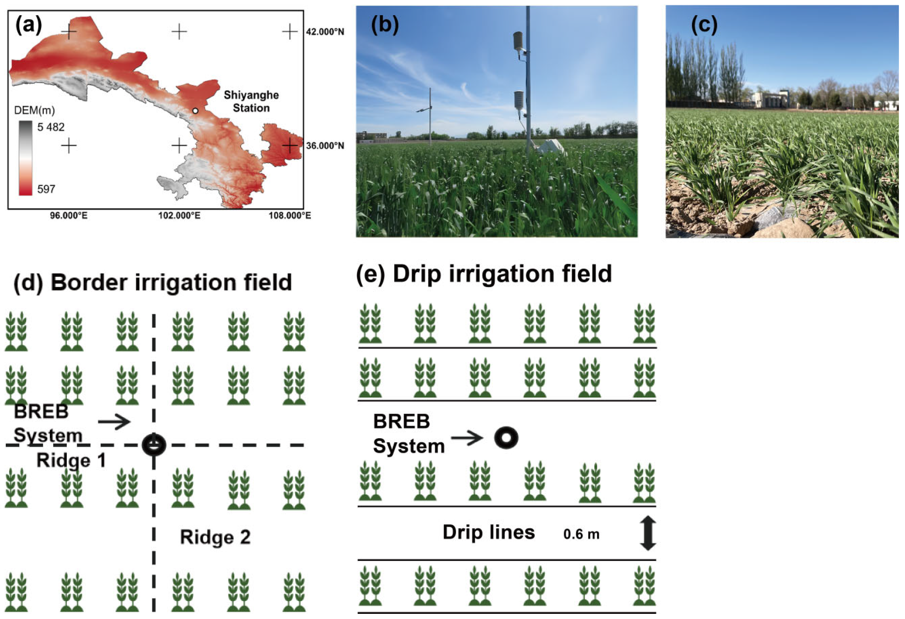
Figure 1. Field experimental location and layout. (a) Location of National Field Scientific Observation and Research Station on Efficient Water Use of Oasis Agriculture in the Hexi Corridor. (b) Layout of Bowen ratio energy balance (BREB) systems. (c) Photo of spring wheat field with plastic mulch drip irrigation. (d) Layout of the border irrigation (BI) field. (e) Layout of the drip irrigation (DI) field.
Agronomy 15 01984 g001
Figure 2. Technical flowchart for obtaining ET using SWAP model and machine learning algorithms.
Agronomy 15 01984 g002
Figure 3. Dynamics in soil water content (SWC) at different layers and different growing stages in two treatments. Note: BI means border irrigation, DI means drip irrigation, (ah) represent the SWC of two treatments on different soil layers from 2017 to 2020, and (i) represents the average SWC of the two treatments during the growing stage. One-way ANOVA with two-sided and post hoc test was conducted for the significance test among different treatments. Different lowercase letters denote significantly different groups of treatments at p < 0.05.
Agronomy 15 01984 g003
Figure 4. ET observed by the BREB system for two types of irrigated fields during different growing stages. Notes: (a) represents BI treatment, (b) represents DI treatment, and (c) represents the average daily ET during the growing stage of BI treatment and DI treatment; DAS represents days after sowing. One-way ANOVA with two-sided and post hoc test was conducted for the significance test among different treatments. Different lowercase letters denote significantly different groups of treatments at p < 0.05.
Agronomy 15 01984 g004
Figure 5. Correlation between ET and its main driving factors based on partial correlation analysis. Notes: (a) represents BI treatment and (b) represents DI treatment. Nore: * indicates statistical significance at p < 0.05; ** indicates statistical significance at p < 0.01.
Agronomy 15 01984 g005
Figure 6. Comparison of observed and simulated ET under BI treatment. Notes: (a) represents the dynamic changes observed in 2017, (b) represents the dynamic changes observed in 2018, (c) represents the dynamic changes observed in 2019, and (d) represents the dynamic changes observed in 2020.
Agronomy 15 01984 g006
Figure 7. Comparison of observed and simulated ET under the DI treatment. Notes: (a) represents the dynamic changes observed in 2017, (b) represents the dynamic changes observed in 2018, (c) represents the dynamic changes observed in 2019, and (d) represents the dynamic changes observed in 2020.
Agronomy 15 01984 g007
Figure 8. Simulation of ET during the growing stage of the spring wheat with RF (a), SVM (b), XGBoost (c), Ridge (d), Stacking (e), and the SWAP model (f) under the BI treatment.
Agronomy 15 01984 g008
Figure 9. Simulation of ET during the growing stage of wheat based with RF (a), SVM (b), XGBoost (c), Ridge (d), Stacking (e), and the SWAP model (f) under the DI treatment.
Agronomy 15 01984 g009
Table 1. Bulk density, field capacity, residual water content, saturated water content, saturated hydraulic conductivity, pH, and soil salt content at different soil depths in DI treatment and BI treatment. Note: DI means drip irrigation; BI means border irrigation.
TreatmentSoil Depths (cm)Bulk Density
(g cm−3)
Field Capacity
(cm3 cm−3)
Residual Water
Content
(cm3 cm−3)
Saturated Water
Content
(cm3 cm−3)
Saturated
Hydraulic Conductivity
(cm d−1)
pHSoil Salt
Content (g kg−1)
DI0–201.410.320.040.4135.848.551.36
20–401.570.310.070.4032.738.771.37
40–601.570.310.060.4230.058.842.62
60–801.510.330.080.4528.668.952.48
80–1001.430.340.110.4328.418.942.26
BI0–201.530.300.040.4436.848.751.17
20–401.560.300.040.4433.658.871.10
40–601.490.320.060.4530.778.911.73
60–801.440.340.080.4524.978.762.61
80–1001.450.350.090.4428.418.842.25
Table 2. The sowing date, harvest date, irrigation amount, irrigation date, fertilization amount, and fertilization date of wheat.
Irrigation MethodIrrigation DateIrrigation Amount/mmFertilization Amount/kg N ha−1Irrigation MethodIrrigation DateIrrigation Amount/mmFertilization Amount/kg N ha−1
DI06/05/20176045BI05/05/201712090
17/05/20176045 26/05/201711762
27/05/20176022.5 13/06/201773
12/06/201757 03/07/201764
23/06/201757
04/07/201741
Sum335112.5 Sum374152
05/05/201810054 05/05/201810082
19/05/20185541 27/05/201811854
28/05/20185541 16/06/2018108
09/06/201855 04/07201890
18/06/201855
29/06/201845
05/07/201845
Sum410136 Sum416136
06/05/20196668 04/05/201998150
19/05/20196668 25/05/201998
30/05/201954 13/06/201984
09/06/201945 06/07/201972
17/06/201937
30/06/201918
09/07/201930
Sum316136 Sum352150
08/05/20206668 07/052020108150
17/05/20206668 29/05/202087
29/05/202050 17/06202076
08/06/202045 07/07/202076
17/06/202035
27/06/202025
07/07/202025
Sum312136 Sum347150
Table 3. Meteorological parameters during the experimental period from 2017 to 2020.
YearMonthu2 (m s−1)Tmax (°C)Tmin (°C)RHmax (%)RHmin (%)P (mm)
201731.114.4−0.373.625.74.2
41.318.53.671.126.122.0
51.125.09.465.820.121.4
60.827.713.074.130.221.8
70.732.216.073.330.87.2
201831.121.92.746.813.20.0
41.017.93.569.626.821.6
50.825.39.462.717.64.6
60.728.713.869.529.18.8
70.529.414.784.839.86.4
201930.616.8−1.845.111.40.0
40.922.05.761.620.07.8
51.022.58.571.229.327.0
60.626.613.480.041.151.6
70.329.613.484.237.923.8
202041.019.93.043.513.70.0
51.223.69.163.724.723.8
60.828.312.971.126.710.8
70.329.314.483.035.623.0
Table 4. Growing stages and GDD of BI and DI fields during the experimental period.
YearGrowing StageBIDaysGDD (°C)DIDaysGDD (°C)
2017Seedling Stage28/03/2017−11/05/201745323.528/03/2017−11/05/201745324.9
Jointing Stage12/05/2017−30/05/201719287.112/05/2017−26/05/201715186.0
Heading Stage31/05/2017−20/06/201721293.927/05/2017−14/06/201719267.0
Filling Stage21/06/2017−05/07/201715238.415/06/2017−29/06/201715319.4
Maturing Stage06/07/2017−21/07/201716309.630/06/2017−15/07/201716408.1
Entire crop season28/03/2017−21/07/20171161452.528/03/2017−15/07/20171101505.4
2018Seedling Stage21/03/2018−09/05/201850402.421/03/2018−09/05/201850406.5
Jointing Stage10/05/2018−27/05/201818225.310/05/2018−23/05/201814176.6
Heading Stage28/05/2018−13/06/201817241.124/05/2018−07/06/201815236.2
Filling Stage14/06/2018−03/07/201820335.908/06/2018−26/06/201819313.9
Maturing Stage04/07/2018−23/07/201820350.227/06/2018−16/07/201820341.7
Entire crop season21/03/2018–23/07/20181251554.921/03/2018−16/07/20181181474.9
2019Seedling Stage25/03/2019−10/05/201947352.925/03/2019−10/05/201947369.2
Jointing Stage11/05/2019−28/05/201918198.511/05/2019−25/05/201915172.4
Heading Stage29/05/2019−17/06/2019 20293.526/05/2019−13/06/201919265.8
Filling Stage18/06/2019−07/07/201920289.914/06/2019−02/07/201919268.1
Maturing Stage08/07/2019−28/07/201921336.303/07/2019−22/07/201920316.8
Entire crop season25/03/2019−28/07/20191261471.125/03/2019−22/07/20191201392.3
2020Seedling Stage02/04/2020−13/05/202042361.302/04/2020−13/05/202042372.5
Jointing Stage14/05/2020−30/05/202017199.314/05/2020−28/05/202015204.3
Heading Stage31/05/2020−18/06/202019279.029/05/2020−15/06/202018251.4
Filling Stage19/06/2020−08/07/202020334.416/06/2020−04/07/202019319.3
Maturing Stage09/07/2020−28/07/202020326.705/07/2020−23/07/202019333.6
Entire crop season02/04/2020−28/07/20201181500.702/04/2020−23/07/20201131481.1
Table 5. Values of ETSWAP and ETBREB during different growing stages under different irrigation methods.
Growing Stage2017201820192020Average
ETBIBREB
(mm)
Seedling109.0103.9105.267.796.5
Jointing129.6130.6119.665.3111.3
Heading133.8123.6135.7102.3123.9
Filling83.5119.5110.295.1102.1
Maturing91.474.8103.244.178.4
All growing stages547.3552.4573.9374.5512.0
ETBISWAP
(mm)
Seedling72.473.260.349.363.8
Jointing106.684.897.478.691.9
Heading113.599.0114.3108.2108.8
Filling90.396.388.0105.995.1
Maturing90.574.089.365.279.8
All growing stages473.3427.3449.3407.2439.3
ETDIBREB
(mm)
Seedling73.1100.183.161.279.4
Jointing74.0103.398.853.282.3
Heading103.383.9142.4101.3107.7
Filling66.0149.7102.086.6101.1
Maturing74.485.095.051.076.4
All growing stages390.8522.0521.3353.3446.9
ETDISWAP
(mm)
Seedling60.555.756.540.053.2
Jointing75.960.181.968.071.5
Heading100.882.2113.1104.9100.3
Filling89.6107.981.697.894.2
Maturing73.091.494.954.778.5
All growing stages399.8397.3428.0365.4397.6
Disclaimer/Publisher’s Note: The statements, opinions and data contained in all publications are solely those of the individual author(s) and contributor(s) and not of MDPI and/or the editor(s). MDPI and/or the editor(s) disclaim responsibility for any injury to people or property resulting from any ideas, methods, instructions or products referred to in the content.